On the Dirichlet-to-Neumann coarse space for solving the Helmholtz problem using domain decomposition
Abstract
We examine the use of the Dirichlet-to-Neumann coarse space within an additive Schwarz method to solve the Helmholtz equation in 2D. In particular, we focus on the selection of how many eigenfunctions should go into the coarse space. We find that wave number independent convergence of a preconditioned iterative method can be achieved in certain special cases with an appropriate and novel choice of threshold in the selection criteria. However, this property is lost in a more general setting, including the heterogeneous problem. Nonetheless, the approach converges in a small number of iterations for the homogeneous problem even for relatively large wave numbers and is robust to the number of subdomains used.
1 Introduction
Within domain decomposition methods, the use of a coarse space as a second level is typically required to provide scalability with respect to the number of subdomains used DoleanEtAl-Book. More recently, coarse spaces have also been designed to provide robustness to model parameters, especially for large contrasts in heterogeneous problems. For example, the GenEO coarse space has been successfully employed for the robust solution of highly heterogeneous elliptic problems SpillaneEtAl-GenEO. One way in which a coarse space can be derived is via solving local eigenvalue problems on subdomains, as is the case for the GenEO method. An earlier approach, having many similarities, is the Dirichlet-to-Neumann (DtN) coarse space NatafEtAl-DtN. We focus on this method which solves eigenvalue problems on the boundary of subdomains related to a Dirichlet-to-Neumann map.
We are interested in using domain decomposition methodology to solve wave propagation problems. In particular, we consider the Helmholtz problem11 1 Note that if then the problem will be ill-posed for certain choices of corresponding to Dirichlet eigenvalues of the corresponding Laplace problem.
| (1a) | ||||||
| (1b) | ||||||
| (1c) | ||||||
with wave number , where and . Such problems arise in many wave propagation and scattering problems in science and engineering, for instance, acoustic and seismic imaging problems. Furthermore, we also consider the heterogeneous problem, in which case varies in the domain . We suppose the variation in stems from the wave speed depending on the heterogeneous media, with the wave number being given by for angular frequency .
The wave number is the key parameter within the Helmholtz equation and as increases the problem becomes more challenging. We are interested in the case when becomes large and so solutions are highly oscillatory. The numerical method employed needs to be able to capture this behaviour, often through an increasing number of grid points, such as a fixed number of points per wavelength. However, typically the number of grid points needs to grow faster than linearly in if accuracy is to be maintained due to the pollution effect BabuskaAndSauter-Pollution. For instance, when using P1 finite elements for the numerical solution of (1), the mesh spacing should grow as . This means very large linear systems must be solved when is large and, since these systems are sparse, iterative methods are most often employed for their solution. However, efficiently solving large discrete Helmholtz systems is challenging since classical iterative methods fail to be effective ErnstAndGander-Helmholtz. As such, we require a more robust iterative solver. Here we consider a restricted additive Schwarz (RAS) method with a Dirichlet-to-Neumann coarse space ConenEtAl-DtN and will be interested in the performance of this solver methodology as increases. We now review the underlying numerical methods we use.
2 Discretisation and solver methodology
To discretise we use finite element methodology, in particular using piecewise linear (P1) finite elements on simplicial meshes. Given a simplicial mesh on a bounded polygonal domain , let be the space of piecewise linear functions on . The P1 finite element solution satisfies the weak formulation , where
| and | (2) |
Using the standard nodal basis for we can represent the solution through its basis coefficients and reduce the problem to solving the complex symmetric linear system where comes from the bilinear form and the linear functional ; see, for example, ConenEtAl-DtN.
To solve the discrete Helmholtz system we utilise a two-level domain decomposition preconditioner within an iterative Krylov method. Since is only complex symmetric rather than Hermitian, we use GMRES as the iterative Krylov method SaadAndSchultz-GMRES. For the domain decomposition, given an overlapping partition of , let represent the matrix form of the restriction onto subdomain . Then the restricted additive Schwarz (RAS) domain decomposition preconditioner is given by
| (3) |
where is the local Dirichlet matrix on and the diagonal matrices are a discrete representation of a partition of unity (see DoleanEtAl-Book); this removes “double counting” in regions of overlap. Note that each subdomain contribution from the sum in (3) can be computed locally in parallel. Using the one-level preconditioner (3) is not sufficient to provide robustness with respect to the number of subdomains used and also becomes much worse when increases. To this end we incorporate a coarse space as a second level within the method.
A coarse space provides a more efficient way to transfer information globally between subdomains, rather than relying solely on local solutions, as in (3). The coarse space constitutes a collection of column vectors , having full column rank. We then utilise the coarse correction operator , where is the coarse space operator, which provides a coarse solution in the space spanned by the columns of . To incorporate the coarse correction we use an adapted deflation (AD) approach given by the two-level preconditioner
| (4) |
To complete the specification, we must choose which vectors go into the coarse space matrix .
3 The Dirichlet-to-Neumann coarse space
We now introduce the Dirichlet-to-Neumann coarse space. The construction is based on solving local eigenvalue problems on subdomain boundaries related to the DtN map. To define this map we first require the Helmholtz extension operator from the boundary of a subdomain .
Let and suppose we have Dirichlet data on , then the Helmholtz extension in is defined as the solution of
| (5a) | ||||||
| (5b) | ||||||
| (5c) | ||||||
where represents the original problem boundary conditions (1b)–(1c). The DtN map takes Dirichlet data on to the corresponding Neumann data, that is
| (6) |
where is the Helmholtz extension defined by (5).
We now seek eigenfunctions of the DtN map locally on each subdomain , given by solving
| (7) |
for eigenfunctions and eigenvalues . To provide functions to go into the coarse space, we take the Helmholtz extension of in and then extend by zero into the whole domain using the partition of unity. For further details and motivation, as well as the discrete formulation of the eigenproblems, see ConenEtAl-DtN.
It remains to determine which eigenfunctions of (7) should be included in the coarse space. Several selection criteria were investigated in ConenEtAl-DtN and it was clear that the best choice was to select eigenvectors corresponding to eigenvalues with the smallest real part. That is, we use a threshold on the abscissa given by
| (8) |
where depends on . In particular, ConenEtAl-DtN advocate the choice . Clearly, the larger is taken, the more eigenfunctions we include in the coarse space, increasing its size and the associated computational cost. However, it is not clear that is necessarily the best choice. We investigate the utility of choosing larger than and will see that, in some cases, taking a slightly larger coarse space can give improved behaviour as the wave number is increased.
4 Numerical results
To investigate the dependence on we use a 2D wave guide problem on the unit square as our model test problem. The Dirichlet condition (1b) is imposed on the left and right boundaries while the Robin condition (1c) is prescribed for the top and bottom boundaries . The right-hand side models a point source at the centre . The wave number is either constant throughout for the homogeneous problem or else where is constant and is piecewise constant as illustrated in Figure 1 for a contrast parameter . These heterogeneous problems model layered media.
To discretise we use a uniform square grid with points in each direction and triangulate with alternating diagonals to form the P1 elements. As we increase we choose in order to ameliorate the pollution effect. To begin with, we use a uniform decomposition into square subdomains and throughout use minimal overlap. All computations are performed using FreeFem (http://freefem.org/), in particular using the ffddm framework. When solving the linear systems we use preconditioned GMRES with the two-level preconditioner (4) incorporating the DtN coarse space with threshold to reach a relative residual tolerance of .
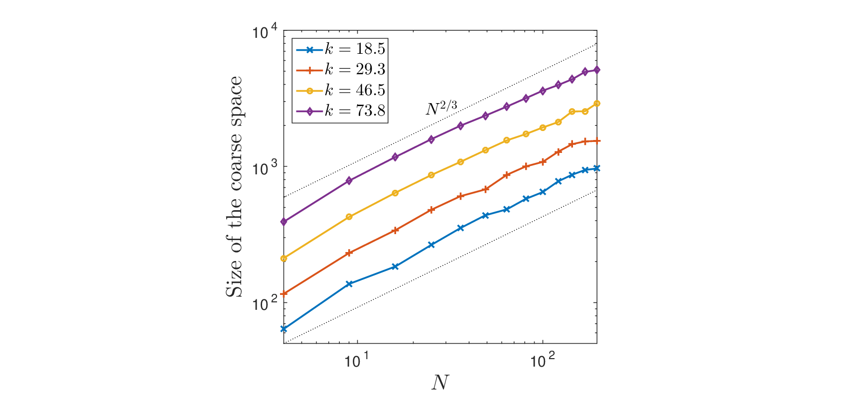
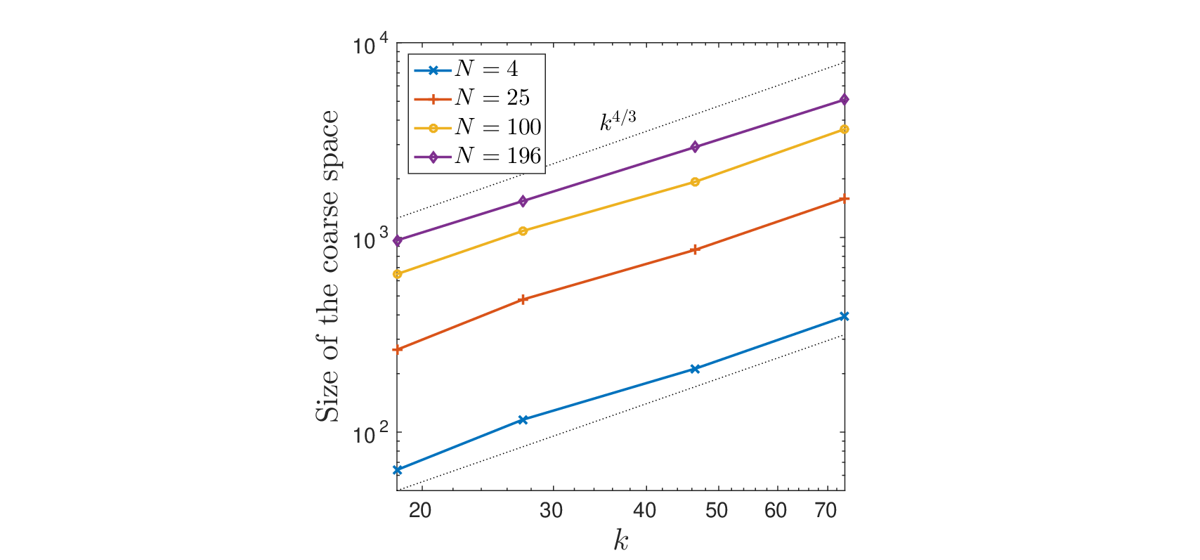
In Table 1 we vary the threshold as powers for the homogeneous problem using a fixed square decomposition. The best choice advocated in ConenEtAl-DtN, namely , succeeds in requiring relatively low iteration counts to reach convergence with a modest size of coarse space. However, we observe that as the wave number increases the number of iterations required also increases, suggesting the approach will begin to struggle if becomes too large. We see from other choices of that taking a larger coarse space reduces the iteration counts. For instance, with the largest wave number tested when the size of the coarse space doubles while the iteration count it cut almost by a factor of three compared to . In fact, there is a qualitative change in behaviour with respect to the wave number , namely independence of the iteration counts to , once becomes large enough, this point being approximately given by . We note that the size of the coarse space is approximately proportional to in the results of Table 1 (see also Figure 2). As such, we see that the coarse space should grow faster than linearly in in order to achieve wave number independent iteration counts for this problem.
| 100 | 18.5 | 12 (144) | 9 (160) | 8 (200) | 7 (240) | 6 (320) | 5 (400) |
|---|---|---|---|---|---|---|---|
| 200 | 29.3 | 16 (215) | 11 (240) | 9 (320) | 7 (434) | 6 (560) | 5 (760) |
| 400 | 46.5 | 18 (299) | 13 (393) | 10 (545) | 7 (784) | 6 (1074) | 4 (1480) |
| 800 | 73.8 | 27 (499) | 18 (674) | 10 (960) | 8 (1376) | 6 (2025) | 4 (2928) |
We now verify that the DtN coarse space provides an approach which is scalable with respect to the number of subdomains . Table 2 details results for a varying number of square subdomains when using a threshold . As well as seeing the iteration counts staying predominantly constant as we increase , they do also as we increase the number of subdomains (aside from a small number of slightly larger outliers). Note that, while the size of the coarse space increases as we increase , approximately at a rate proportional to as shown in Figure 2 (in fact, independent of our choice of ), the number of eigenfunctions required per subdomain decreases with . This means the solution of each eigenproblem is much cheaper for large as they are of smaller size and we require fewer eigenfunctions.
| 4 | 9 | 16 | 25 | 36 | 49 | 64 | 81 | 100 | 121 | 144 | 169 | 196 | ||
|---|---|---|---|---|---|---|---|---|---|---|---|---|---|---|
| 100 | 18.5 | 6 | 6 | 8 | 6 | 6 | 6 | 6 | 6 | 6 | 6 | 6 | 7 | 7 |
| 200 | 29.3 | 6 | 13 | 8 | 6 | 6 | 17 | 7 | 7 | 7 | 7 | 7 | 7 | 7 |
| 400 | 46.5 | 7 | 11 | 7 | 7 | 7 | 7 | 7 | 7 | 10 | 20 | 7 | 7 | 7 |
| 800 | 73.8 | 7 | 9 | 9 | 7 | 7 | 7 | 7 | 7 | 7 | 7 | 8 | 7 | 7 |
We now turn our attention to the heterogeneous case. Table 3 (left) gives results for the alternating layers wave guide problem (see Figure 1a) for varying angular frequency , contrast in wave speed , and number of subdomains when using in subdomain . The picture painted is now rather different from the homogeneous case. While for some choices of iteration counts remain robust to wave number, in general they degrade as increases. The best results are for , , and (powers of 2) while the poorest are with large . More generally, if the subdomains are close to being aligned with the jumps in we obtain better results, otherwise robustness is lost. We note, however, that iteration counts are robust to large contrasts . We confirm that the disparate trends observed for the alternating layers problem are due to the geometrical aspects of the problem by considering instead the diagonal layers problem (see Figure 1b). Results for the diagonal layers problem are given in Table 3 (right) and now show that any robustness to the wave number is, in general, lost for the heterogeneous problem. We note that increasing the threshold to does not improve this assessment. Nonetheless, the DtN approach remains robust to increasing the number of subdomains .
| Alternating layers problem | Diagonal layers problem | |||||||||||||||||||||||
| 4 | 9 | 16 | 25 | 36 | 49 | 64 | 81 | 100 | 121 | 144 | 4 | 9 | 16 | 25 | 36 | 49 | 64 | 81 | 100 | 121 | 144 | |||
| 10 | 6 | 6 | 7 | 6 | 6 | 14 | 6 | 16 | 13 | 17 | 13 | 7 | 12 | 15 | 18 | 18 | 18 | 18 | 18 | 17 | 17 | 18 | ||
| 100 | 18.5 | 100 | 6 | 6 | 7 | 6 | 6 | 14 | 6 | 16 | 13 | 17 | 13 | 11 | 20 | 21 | 20 | 19 | 19 | 18 | 18 | 17 | 16 | 16 |
| 1000 | 6 | 6 | 7 | 6 | 6 | 14 | 6 | 16 | 13 | 17 | 13 | 11 | 20 | 21 | 20 | 19 | 19 | 18 | 18 | 17 | 16 | 16 | ||
| 10 | 8 | 8 | 9 | 8 | 9 | 29 | 9 | 29 | 25 | 32 | 22 | 9 | 17 | 20 | 19 | 19 | 23 | 21 | 28 | 28 | 28 | 28 | ||
| 200 | 29.3 | 100 | 8 | 7 | 9 | 8 | 8 | 28 | 8 | 28 | 23 | 30 | 20 | 16 | 28 | 30 | 30 | 28 | 29 | 27 | 27 | 25 | 25 | 24 |
| 1000 | 8 | 7 | 9 | 8 | 8 | 28 | 8 | 28 | 23 | 30 | 20 | 16 | 28 | 30 | 29 | 28 | 29 | 27 | 27 | 25 | 25 | 24 | ||
| 10 | 9 | 7 | 7 | 7 | 7 | 25 | 7 | 29 | 25 | 45 | 22 | 10 | 18 | 20 | 25 | 26 | 26 | 25 | 26 | 26 | 32 | 29 | ||
| 400 | 46.5 | 100 | 9 | 7 | 7 | 7 | 7 | 24 | 7 | 28 | 24 | 44 | 22 | 22 | 39 | 43 | 43 | 40 | 40 | 39 | 37 | 37 | 39 | 35 |
| 1000 | 9 | 7 | 7 | 7 | 7 | 24 | 7 | 28 | 24 | 44 | 22 | 22 | 38 | 43 | 42 | 40 | 40 | 39 | 37 | 37 | 39 | 34 | ||
| 10 | 8 | 10 | 8 | 11 | 9 | 30 | 8 | 34 | 27 | 36 | 33 | 11 | 19 | 24 | 29 | 28 | 30 | 31 | 34 | 37 | 40 | 41 | ||
| 800 | 73.8 | 100 | 8 | 10 | 8 | 11 | 9 | 38 | 8 | 43 | 33 | 39 | 31 | 32 | 52 | 62 | 61 | 60 | 58 | 58 | 54 | 53 | 53 | 51 |
| 1000 | 8 | 10 | 8 | 11 | 9 | 38 | 8 | 43 | 33 | 39 | 31 | 32 | 55 | 60 | 60 | 59 | 56 | 56 | 54 | 52 | 51 | 49 | ||
We now show that the sensitivity of the DtN approach is not solely due to the heterogeneity of the media by reconsidering the homogeneous problem but using non-uniform subdomains, which we compute using METIS. Results for this case are given in Table 4 where we see a slow but definite increase in iteration counts as increases. Again, we see robustness to the number of subdomains but lose robustness to the wave number. Note that this persists even for . Nonetheless, in our DtN approach we still have rather few GMRES iterations required to compute the solution when is relatively large (in this case up to ).
| 4 | 9 | 16 | 25 | 36 | 49 | 64 | 81 | 100 | 121 | 144 | 169 | 196 | ||
|---|---|---|---|---|---|---|---|---|---|---|---|---|---|---|
| 100 | 18.5 | 7 | 7 | 11 | 7 | 7 | 7 | 7 | 7 | 7 | 7 | 7 | 7 | 7 |
| 200 | 29.3 | 8 | 9 | 10 | 7 | 11 | 9 | 7 | 7 | 7 | 7 | 7 | 7 | 7 |
| 400 | 46.5 | 8 | 10 | 10 | 13 | 14 | 16 | 9 | 14 | 15 | 9 | 8 | 8 | 8 |
| 800 | 73.8 | 8 | 10 | 12 | 12 | 15 | 15 | 13 | 17 | 11 | 14 | 10 | 12 | 17 |
| 1600 | 117.2 | 10 | 12 | 12 | 15 | 16 | 16 | 17 | 17 | 17 | 16 | 16 | 16 | 16 |
| 100 | 18.5 | 75 | 158 | 219 | 303 | 397 | 476 | 558 | 644 | 740 | 829 | 923 | 1024 | 1118 |
| 200 | 29.3 | 135 | 282 | 418 | 558 | 677 | 860 | 1003 | 1123 | 1275 | 1435 | 1588 | 1731 | 1867 |
| 400 | 46.5 | 241 | 516 | 751 | 1001 | 1291 | 1569 | 1818 | 2048 | 2294 | 2596 | 2850 | 3145 | 3366 |
| 800 | 73.8 | 481 | 979 | 1446 | 1919 | 2378 | 2844 | 3261 | 3753 | 4291 | 4651 | 5246 | 5720 | 6126 |
| 1600 | 117.2 | 925 | 1857 | 2639 | 3566 | 4408 | 5244 | 6201 | 7008 | 7909 | 8770 | 9563 | 10448 | 11402 |
5 Conclusions
In this work we have investigated a two-level domain decomposition approach to solving the heterogeneous Helmholtz equation. Our focus has been on the Dirichlet-to-Neumann coarse space and how the approach depends on the threshold to select which eigenfunctions go into the coarse space. We have seen that the threshold in ConenEtAl-DtN can be improved in order to give wave number independent convergence with only moderate added cost due to the larger coarse space. However, this is only true for the homogeneous problem with sufficiently uniform subdomains. In particular, convergence depends on the wave number for a general heterogeneous problem.
In order to obtain fully wave number independent convergence for Helmholtz problems, a stronger coarse space is needed. A recent approach that achieves this, based on a related GenEO-type method, can be found in BootlandEtAl-H-GenEO.
References
- (1) Babuška, I.M., Sauter, S.A.: Is the pollution effect of the FEM avoidable for the Helmholtz equation considering high wave numbers? SIAM J. Numer. Anal. 34(6), 2392–2423 (1997)
- (2) Bootland, N., Dolean, V., Jolivet, P.: A GenEO-type coarse space for heterogeneous Helmholtz problems (2019). In preparation
- (3) Conen, L., Dolean, V., Krause, R., Nataf, F.: A coarse space for heterogeneous Helmholtz problems based on the Dirichlet-to-Neumann operator. J. Comput. Appl. Math. 271, 83–99 (2014)
- (4) Dolean, V., Jolivet, P., Nataf, F.: An Introduction to Domain Decomposition Methods: Algorithms, Theory, and Parallel Implementation, vol. 144. SIAM (2015)
- (5) Ernst, O.G., Gander, M.J.: Why it is difficult to solve Helmholtz problems with classical iterative methods. In: I.G. Graham, T.Y. Hou, O. Lakkis, R. Scheichl (eds.) Numerical Analysis of Multiscale Problems, pp. 325–363. Springer (2012)
- (6) Nataf, F., Xiang, H., Dolean, V., Spillane, N.: A coarse space construction based on local Dirichlet-to-Neumann maps. SIAM J. Sci. Comput. 33(4), 1623–1642 (2011)
- (7) Saad, Y., Schultz, M.H.: GMRES: A generalized minimal residual algorithm for solving nonsymmetric linear systems. SIAM J. Sci. Stat. Comput. 7(3), 856–869 (1986)
- (8) Spillane, N., Dolean, V., Hauret, P., Nataf, F., Pechstein, C., Scheichl, R.: Abstract robust coarse spaces for systems of PDEs via generalized eigenproblems in the overlaps. Numer. Math. 126(4), 741–770 (2014)