Measurement of the branching fraction for the decay $K_{S}\to\pi\mu\nu$ with the KLOE detector
The KLOE-2 Collaboration

The branching fraction for semileptonic decays of charged and neutral kaons together with the lifetime measurements are used to determine the $|V_{us}|$ element of the Cabibbo–Kobayashi–Maskawa quark mixing matrix. The relation among the matrix elements of the first row, $|V_{ud}|^{2}+|V_{us}|^{2}+|V_{ub}|^{2}=1$, provides the most stringent test of the unitarity of the quark mixing matrix. Different factors contribute to the uncertainty in determining $|V_{us}|$ from kaon decays [1, 2, 3] and among the six semileptonic decays the contribution of the lifetime uncertainty is smallest for the $K_{S}$ meson. Nevertheless, given the lack of pure high-intensity $K_{S}$ meson beams contrary to the case of $K^{\pm}$ and $K_{L}$ mesons, the $K_{S}\to\pi e\nu$ decay provides the least precise determination of $|V_{us}|$, and the branching fraction $\mathcal{B}(K_{S}\to\pi\mu\nu)$ has not yet been measured. Measurement of this decay mode allows an independent determination of $|V_{us}|$ and to extend the test of lepton-flavour universality to $K_{S}$ semileptonic decays by comparison with the expected value of $(4.69\pm 0.06)\times 10^{-4}$ [4] derived from $\mathcal{B}(K_{S}\to\pi e\nu)$.

We present a measurement of the $K_{S}\to\pi\mu\nu$ branching fraction performed by the KLOE experiment at the DA$\Phi$NE $\phi$–factory of the Frascati National Laboratory based on an integrated luminosity of 1.6 fb^-1. DA$\Phi$NE [5] is an electron–positron collider running at the centre-of-mass energy of 1.02 GeV colliding $e^{+}$ and $e^{-}$ beams at an angle of $\pi$$-$0.025 rad and with a bunch-crossing period of 2.71 ns. The $\phi$ mesons are produced with a small transverse momentum of 13 MeV and $K_{L}$–$K_{S}$ pairs are produced almost back-to-back with a cross section times the $\phi\to K_{L}K_{S}$ branching fraction of about 1 $\mu$b. The beam energy, the energy spread, the beams transverse momentum and the position of the interaction point are measured using Bhabha scattering events [6].

The $K_{S}$ ($K_{L}$) mesons are identified (tagged) by the observation of a $K_{L}$ ($K_{S}$) meson in the opposite hemisphere. This tagging procedure allows the selection efficiency for $K_{S}\to\pi\mu\nu$ to be evaluated with good accuracy using a sample of the abundant decay $K_{L}\to\pi\mu\nu$ tagged by the detection of $K_{S}\to\pi^{+}\pi^{-}$ decays. The branching fraction is extracted normalising the number of $K_{S}\to\pi\mu\nu$ events to the number of $K_{S}\to\pi^{+}\pi^{-}$ events recorded in the same dataset.

The detector¹¹ 1 KLOE uses a coordinate system where the $z$ axis is the bisector of the electron and positron beams, $x$ and $y$ axes define the transverse plane, the polar angle is relative to the $z$ axis. consists of a large-volume cylindrical drift chamber, surrounded by a lead/scintillating fibers finely-segmented calorimeter. A superconducting coil around the calorimeter provides a 0.52 T axial magnetic field. The beam pipe at the interaction region is spherical in shape with 10 cm radius, made of a 0.5 mm thick beryllium-aluminum alloy. Final-focus quadrupoles are located at $\pm$50 cm from the interaction region. Two small lead/scintillating-tile calorimeters [7] are wrapped around the quadrupoles.

The drift chamber [8], 4 m in diameter and 3.3 m long, has 12582 drift cells arranged in 58 concentric rings with alternating stereo angles and is filled with a low-density gas mixture of 90% helium–10% isobutane. The chamber shell is made of carbon fiber-epoxy composite with an internal wall of 1.1 mm thickness at 25 cm radius. The spatial resolution is $\sigma_{xy}=$ 0.15 mm and $\sigma_{z}=$ 2 mm in the transverse and longitudinal projections, respectively. The momentum resolution is $\sigma_{p_{\rm T}}/p_{\rm T}=0.4\%$, tracks vertices are reconstructed with a spatial resolution of about 3 mm.

The calorimeter [9] is divided into a barrel and two endcaps and covers 98% of the solid angle. The readout granularity is 4.4$\times$4.4 cm², for a total of 2440 cells arranged in five layers. Each cell is read out at both ends by photomultipliers. The energy deposits are obtained from signal amplitudes while the arrival time and the position along the fibers are obtained from time differences between the two signals. Cells close in time and space are grouped into energy clusters. The cluster energy $E$ is the sum of the cell energies, the cluster time and position are energy-weighted averages. Energy and time resolutions are $\sigma_{E}/E=0.057/\sqrt{E\ {\rm(GeV)}}$ and $\sigma_{t}=54\ {\rm ps}/\sqrt{E\ {\rm(GeV)}}\oplus 100$ ps, respectively. The cluster spatial resolution is $\sigma_{\parallel}=1.4\ {\rm cm}/\sqrt{E\ {\rm(GeV)}}$ along the fibers and $\sigma_{\perp}=1.3$ cm in the orthogonal direction.

The first-level trigger [10] uses both the calorimeter and the drift chamber information; the calorimeter trigger requires two energy deposits with $E>50$ MeV in the barrel and $E>150$ MeV in the endcaps; the drift chamber trigger is based on the number and topology of hit drift cells. A second-level cosmic-ray veto rejects events with at least two energy deposits above 30 MeV in the outermost calorimeter layer. The trigger time is determined by the first particle reaching the calorimeter and is synchronised with the DA$\Phi$NE radio frequency signal. The time interval between bunch crossings is smaller than the time spread of the signals produced by the particles, thus the time of the bunch crossing originating the event, T₀, is determined after event reconstruction and all the times related to that event are shifted accordingly. Data for reconstruction are selected by an on-line filter [11] to reject beam backgrounds. The filter also records the events into different output files for analysis according to their properties and topology (event classification), 5% of the events are recorded without applying the filter to control the efficiency of the event classification.

Processes of interest for the analysis are simulated with the GEANFI Monte Carlo (MC) program [11] for an integrated luminosity equal to that of the data. All $\phi$ decays are generated according to their branching fractions as well as other final states produced in $e^{+}e^{-}$ annihilation. The operating conditions of DA$\Phi$NE during data taking as well as measurements of beam parameters are included in the MC on a run-by-run basis. Calorimeter energy deposits and drift chamber hits from beam background acquired with a random trigger are overlaid onto the simulated events. The simulated events are processed with the same reconstruction algorithms as the data.

Kaons from $\phi$-meson decays are emitted in two opposite hemispheres with mean decay path $\lambda_{S}=5.9$ mm and $\lambda_{L}=3.4$ m, thus about 50% of $K_{L}$ mesons reach the calorimeter before decaying. The velocity of the $K_{L}$ in the $\phi$ reference system is $\beta^{*}=0.22$. $K_{S}$ mesons are tagged by $K_{L}$ interactions in the calorimeter, named $K_{L}$-crash in the following, with a clear signature of a late signal of about 25 ns not associated to tracks. The following requirements are applied to select $K_{L}$-crash:

• 1.

  a cluster with energy $E_{\rm clu}>100$ MeV not associated to tracks (neutral cluster); the centroid of the neutral cluster defines the $K_{L}$ direction with a resolution of $\sim$1^∘;

• 2.

  polar angle of the neutral cluster $15^{\circ}<\theta_{\rm clu}<165^{\circ}$ to suppress small-angle beam backgrounds;

• 3.

  $0.17<\beta^{*}<0.28$ for the velocity in the $\phi$ reference system of the particle originating the neutral cluster; $\beta^{*}$ is obtained from the velocity in the laboratory system, $\beta=r_{\rm clu}/ct_{\rm clu}$, with $t_{\rm clu}$ being the cluster time and $r_{\rm clu}$ the distance from the nominal interaction point, the $\phi$ transverse momentum determined run-by-run and the angle between the $\phi$ momentum and the $K_{L}$-crash direction.

Assuming the neutral kaon mass, the $K_{S}$ 4-momentum is defined by the $K_{L}$-crash direction and the $\phi$ 4-momentum: $P_{K_{S}}=P_{\phi}-P_{K_{L}}$.

The $K_{S}\to\pi\mu\nu$ candidates are selected requiring two tracks of opposite curvature forming a vertex inside the cylinder defined by

In case more than one vertex is found, the closest to the interaction region is chosen. The above requirements define the event preselection.

After preselection, the data sample contains about 300 million events and its composition, as evaluated by simulation, is shown in Table 1. The large majority of events are $K_{S}\to\pi^{+}\pi^{-}$ decays, and there is also a large contribution from $\phi\to K^{+}K^{-}$ events where one kaon or its decay products generate a fake $K_{L}$-crash and the other kaon decays early into $\pi^{\pm}\pi^{0}$.

The distribution of $\beta^{*}$ is shown in Figure 1 for data and simulated events. Two peaks are visible, the first is associated to events triggered by photons or electrons, and the second to events triggered by charged pions. The trigger is synchronised with the bunch crossing and the time difference between a photon (or electron) and a pion (or muon) arriving at the calorimeter corresponds to a time shift of about one bunch-crossing.

The selection of signal events is performed in two steps; first a selection based on the event kinematics using only tracking variables and then a selection based on the time-of-flight measured with the calorimeter. The two groups of variables are uncorrelated. In order to assign a time to the particles each track is associated to a cluster. The track-to-cluster association (TCA) is applied as follows: for each track connected to the vertex a cluster with $E_{\rm clu}>20$ MeV and $15^{\circ}<\theta_{\rm clu}<165^{\circ}$ is required whose centroid is within 60 cm of the track extrapolation to the calorimeter front surface. The event is retained only if TCA is satisfied by both tracks.

Five variables with good discriminating power against background are used in a multivariate analysis. A boosted decision tree (BDT) classifier is built with the following variables:

• $\vec{p}_{1},\vec{p}_{2}$

  : the tracks momenta;

• $\alpha_{1,2}$

  : the angle at the vertex between the two momenta in the $K_{S}$ reference system;

• $\alpha_{SL}$

  : the angle between $\vec{p}_{\rm sum}=\vec{p}_{1}+\vec{p}_{2}$ and the $K_{L}$-crash direction;

• $\Delta p$

  : the difference between $|\vec{p}_{\rm sum}|$ and the absolute value $|\vec{p}_{K_{S}}|$ of the $K_{S}$ momentum determined using the tagging $K_{L}$;

• $m_{\pi\pi}$

  : the invariant mass reconstructed from $\vec{p}_{1}$ and $\vec{p}_{2}$, in the hypothesis of charged-pion mass.

The distributions of the variables are shown in Figure 2 for data and simulated events.

After preselection two cuts are applied to suppress the background in the tails of the distributions:

The training of the BDT classifier is done on a simulated sample of 5,000 $K_{S}\to\pi\mu\nu$ events and a sample of 50,000 background events; samples of the same size are used for the test. After training and test the classification is run on all events of the MC and data sample. The distribution of the BDT classifier output is shown in Figure 3 for data and simulated events. The data distribution is well reproduced by simulation in the region populated by the signal. To suppress the large background of $K_{S}\to\pi^{+}\pi^{-}$ and $\phi\to K^{+}K^{-}$ events, a cut is applied

chosen to maximise the ratio $S/\sqrt{S+B}$ where $S$ and $B$ are the signal and background yields.

The selected events contain $\pi\pi$, $K\pi$, $e\pi$ track pairs for the main backgrounds and $\mu\pi$ for the signal. A selection based on time-of-flight measurement is performed to identify $\mu\pi$ pairs. For each track associated to a cluster, the difference between the time measured by the calorimeter and the time-of-flight measured along the particle trajectory

is computed, where $t_{{\rm clu},i}$ is the time of the cluster associated to track $i$, $L_{i}$ is the length of the track, and $\beta_{i}=p_{i}/\sqrt{p_{i}^{2}+m_{i}^{2}}$ is function of the mass hypothesis for track $i$. To reduce the uncertainty due to the T₀ determination, the difference

is used to determine the mass assignment to the tracks. The $\pi\pi$ hypothesis is tested first, the distribution of $\delta t_{\pi\pi}=\delta t_{1,\pi}-\delta t_{2,\pi}$ is shown in Figure 4(left). A fair agreement is observed between data and simulation, the $K_{S}\to\pi\mu\nu$ and $K_{S}\to\pi e\nu$ distributions are well separated and the $K^{+}K^{-}$ background is isolated in the tails of the distribution, however the signal is hidden under a large $K_{S}\to\pi^{+}\pi^{-}$ background. To reduce the background a cut is applied

The $\pi\mu$ hypothesis is tested by assuming the pion and muon mass for either track

The two-dimensional $(\delta t_{\pi\mu},\delta t_{\mu\pi})$ distribution for simulated signal events shows that the correct mass assignment corresponds to the smaller absolute value of the two hypotheses. The distribution of the signed value of $\delta t_{\mu}={\rm min}\left[|\delta t_{\pi\mu}|,|\delta t_{\mu\pi}|\right]$ is shown in Figure 4(right) for data and simulated events. The distribution for the signal is narrow and peaked at zero while it is broader for the backgrounds. A final cut is applied

The number of surviving events in the data sample is 38686 and its composition as evaluated by simulation is listed in Table 2. After the mass assignment to the two tracks the invariant mass of the charged particle identified as the muon is evaluated as

with $p_{\rm miss}^{2}=(\vec{p}_{K_{S}}-\vec{p}_{\pi}-\vec{p}_{\mu})^{2}$, $E_{K_{S}}$ and $\vec{p}_{K_{S}}$ being the energy and momentum reconstructed using the tagging $K_{L}$, and $\vec{p}_{\pi}$, $\vec{p}_{\mu}$, the momenta of the candidate pion and muon track.

The number of signal events is extracted with a fit to the $m_{\mu}^{2}$ distribution with the MC shapes of three components: $K_{S}\to\pi\mu\nu$, $K_{S}\to\pi^{+}\pi^{-}$ and the sum of all other backgrounds. The fit is performed in the range $-6000<m^{2}_{\mu}<24000$ MeV² with 48 degrees of freedom. The third component, which is peaked around $m_{e}^{2}$, is constrained to a negligible value by the fit. Figure 5 shows the distribution of $m_{\mu}^{2}$ for data, simulated events and the fit, and Table 3 presents the result of the fit. The number of signal events is

The normalisation sample of $K_{S}\to\pi^{+}\pi^{-}$ events is selected by requiring $140<p<280$ MeV for both tracks (Figure 2). This requirement selects $N_{\pi\pi}=(282.314\pm 0.017)\times 10^{6}$ events with a purity of 99.9% as determined by simulation.

The branching fraction for the $K_{S}\to\pi\mu\nu$ decay is evaluated as

where $N_{\pi\mu\nu}$ and $N_{\pi\pi}$ are the numbers of $K_{S}\to\pi\mu\nu$ and $K_{S}\to\pi^{+}\pi^{-}$ events, $\epsilon_{\pi\mu\nu}$ and $\epsilon_{\pi\pi}$ are the respective selection efficiencies, and $R_{\epsilon}$ is the ratio of the efficiencies for the trigger, on-line filter and preselection for the two decays.

The signal selection efficiency is determined with $K_{L}\to\pi\mu\nu$ control samples (CS) and evaluated as

where $\epsilon_{\rm CS}$ is the efficiency of the control sample and $\epsilon^{\rm MC}_{\pi\mu\nu}$, $\epsilon^{\rm MC}_{\rm CS}$ are the efficiencies obtained from simulation for the signal and control samples, respectively.

The $K_{L}\to\pi\mu\nu$ decay [12, 13] is kinematically identical to the signal, the only difference being the much longer decay path. For the control sample the tagging is done with $K_{S}\to\pi^{+}\pi^{-}$ decays, preselected in the same way as for the signal sample with the addional cut $|m_{\pi\pi}-m_{K^{0}}|<15$ MeV to increase the purity. The radial distance of the $K_{L}$ vertex is required to be smaller than 5 cm to match the signal selection, but greater than 1 cm to minimise the ambiguity in identifying the $K_{L}$ and $K_{S}$ vertices. The control sample is composed mainly of $K_{L}\to\pi e\nu$ , $K_{L}\to\pi^{+}\pi^{-}\pi^{0}$ and $K_{L}\to\pi\mu\nu$ decays, while most of $K_{L}\to\pi^{0}\pi^{0}\pi^{0}$ decays are rejected by the requirement of two tracks. The distribution of the missing mass, $m^{2}_{\rm miss}$, of the two tracks connected to the $K_{L}$ vertex, assigning the charged-pion mass, shows a narrow isolated peak at the $\pi^{0}$ mass; a cut $m^{2}_{\rm miss}<15000$ MeV² efficiently rejects the $K_{L}\to\pi^{+}\pi^{-}\pi^{0}$ decays. The number of events in the control sample is 911757.

In order to evaluate the signal selection efficiency, two control samples are used, one selected based on kinematic variables and the other based on time-of-flight (TOF), the two groups of variables being largely uncorrelated.

The control sample for evaluating the efficiencies of the selection with kinematic variables and BDT classifier is selected applying a cut on the two-dimensional $(\delta t_{\pi\mu},\delta t_{\mu\pi})$ distribution that removes most of the $K_{L}\to\pi e\nu$ events. The purity of the sample as determined with simulation is 86%. The resolutions in the measurement of the tagging $K_{S}$ (control sample) are similar to those of the tagging $K_{L}$ (signal sample) and the same BDT classifier is used for both samples. The BDT MC distributions for the signal and control sample are compared in Figure 6(left). Applying to the control sample the same selections as for the signal, the efficiencies evaluated with Eq. (7) are

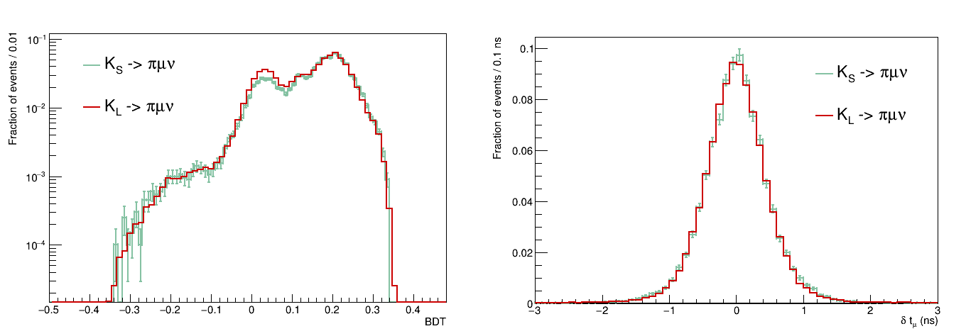
To evaluate TCA and TOF efficiencies for the signal, the T0 determination using the earlier among the two clusters associated with the $K_{S}$ decay has to be considered. The control sample selection therefore requires the earliest cluster to be associated with one of charged secondary particles from $K_{L}$ decay and a cut on the $(m_{\pi\pi},m^{2}_{\rm miss})$ distribution to reject $K_{L}\to\pi e\nu$ events. The purity of the sample as determined with simulation is 87%. The MC distributions of $\delta t_{\mu}$ for the signal and control sample are compared in Figure 6(right). Applying to the control sample the analysis procedure as for the signal the efficiencies evaluated with Eq. (7) are

The correction factors in Eq. (7) differ from one by less than 10% but for $\epsilon$(TOF) where it differs by 20%.

The tails of the $m^{2}_{\mu}$ distribution in Figure 5(left) are not included in the fit to improve its stability, the relative efficiency is $0.991\pm 0.001$.

The signal selection efficiencies are summarised in Table 4 where only the statistical errors are shown. Combining the values accounting for the correlation of the control samples we obtain $\epsilon_{\pi\mu\nu}=0.0552\pm 0.0005$.

The ratio $R_{\epsilon}$ in Eq. (6) accounts for several effects all depending on the global properties of the event: trigger, on-line filter, event classification, T₀ determination, $K_{L}$-crash and $K_{S}$ identification. The various contributions to $R_{\epsilon}$ evaluated with simulation are listed in Table 5 where only the statistical errors are shown.

The efficiency of the $K_{S}\to\pi^{+}\pi^{-}$ normalisation sample is measured using the preselected data by varying the cut on the vertex transverse position, as in Eq. (1), in 1 cm steps from $\rho^{\rm max}_{\rm vtx}=1$ cm to $\rho^{\rm max}_{\rm vtx}=4$ cm, based on the observation that $\rho_{\rm vtx}$ and the tracks momenta are very loosely correlated. Using Eq. (7) and extrapolating to $\rho^{\rm max}_{\rm vtx}=5$ cm the efficiency is $\epsilon_{\pi\pi}=(96.569\pm 0.004)\%$. Alternatively, the efficiency is evaluated using the $K_{S}\to\pi^{+}\pi^{-}$ data sample (with $\rho^{\rm max}_{\rm vtx}=5$ cm ): $\epsilon_{\pi\pi}=(96.657\pm 0.002)\%$. The latter value is used as the efficiency and the difference between the two values is taken as systematic uncertainty. The number of $K_{S}\to\pi^{+}\pi^{-}$ events corrected for the efficiency is

Three main systematic uncertainties affect the signal count: BDT and time-of-flight selection, and the $m^{2}_{\mu}$ fit.

The distributions of the BDT classifier output for the data and simulated signal and control sample events are in good agreement as shown in Figures 3 and 6. The resolution of the BDT variable predicted by simulation comparing the reconstructed events with those at generation level is $\sigma_{\rm BDT}=0.005$. The analysis is repeated varying the BDT cut of Eq. (3), the number of signal events is found to be stable and the rms value of the differences corresponds to a relative uncertainty of 0.3%.

The main source of uncertainty in the TOF selection is the cut on $\delta t_{\pi\pi}$ in Eq. (4) because the signal and background distributions in Figure 4(left) are steep and with opposite slopes; the subsequent selection on $\delta t_{\mu}$ in Eq. (5) has a minor effect. The resolution of the $\delta t_{\pi\pi}$ variable evaluated with simulation and $K_{S}\to\pi^{+}\pi^{-}$ data control samples is $0.27$ ns. The analysis is repeated varying the $\delta t_{\pi\pi}$ lower cut in the range 0.5–1.25 ns, the rms value of the differences corresponds to a relative uncertainty of 3.0%. This is the main systematic uncertainty affecting the measurement.

The fit to the $m_{\mu^{2}}$ distribution in Figure 5 is repeated varying the range and the bin size. The relative systematic uncertainty on the number of events is 0.3% obtained shifting the range by five bins on either side and increasing the bin size by a factor of two.

The statistical uncertainties of the simulation signal and control samples, and of the data control sample contribute with a relative uncertainty of 0.8% (Table 4).

The dependence of $R_{\epsilon}$ on systematic effects has been studied in previous analyses for different $K_{S}$ decays selected with the $K_{L}$-crash method: $K_{S}\to\pi^{+}\pi^{-}$ and $K_{S}\to\pi^{0}\pi^{0}$ [14], and $K_{S}\to\pi e\nu$ [15]. The systematic uncertainties are evaluated by a comparison of data with simulation, as described in the following.

Trigger – Two triggers are used for recording the events, the calorimeter trigger and the drift chamber trigger. The validation of the MC relative efficiency is derived from the comparison of the single-trigger and coincidence rates with the data. The data over MC ratio is 0.999 with negligible error.

On-line filter and event classification – The event classification produces different streams for the analyses. The $K_{L}K_{S}$ stream selects events based on the properties of $K_{S}$ and $K_{L}$ decays. In more than 99% of the cases the events are selected based on the $K_{S}$ decay topology and the $K_{L}$-crash signature and differences between MC and data are accounted for in the systematic uncertainties derived below for the $K_{S}$ identification and $K_{L}$-crash.

T₀ – The systematic uncertainty is evaluated analising the data and MC T₀ distributions for the decays with the most different timing properties: $K_{S}\to\pi^{+}\pi^{-}$ and $K_{S}\to\pi^{0}\pi^{0}$ [14]. The data over MC ratios is one with an uncertainty of less than 0.1%.

$K_{L}$-crash and $\beta^{*}$ selection – The systematic uncertainty is evaluated comparing data and simulated events tagged by $K_{S}\to\pi^{+}\pi^{-}$ and $K_{S}\to\pi^{0}\pi^{0}$ decays which have different timing and topology characteristics. The data over MC ratio is 1.001 with negligible error.

$K_{S}$ identification – The systematic uncertainty due to the requirement of two tracks forming a vertex in the cylinder defined by Eq. (1) is evaluated separately for signal and normalisation samples. The first is evaluated with $K_{L}\to\pi\mu\nu$ events selected with the same vertex requirements as for the signal but tagged by $K_{S}\to\pi^{0}\pi^{0}$ decays. For the $K_{S}\to\pi^{+}\pi^{-}$ sample the efficiency is evaluated by tagging with $K_{L}$-crash and removing the requirement of the vertex. Combining the two values gives a data over MC ratio of 1.002 $\pm$ 0.017 where the error is due to the purity of the samples.

The $R_{\epsilon}$ total systematic uncertainty is estimated by combining the data over MC ratios and amounts to 1.7%.

Including the systematic uncertainties the factors in Eq. (6) are:

All systematic uncertainties are summarised in Table 6.

From Eq. (6) with $N_{\pi\mu\nu}=7223\pm 180$, $N_{\pi\pi}/\epsilon_{\pi\pi}=(292.08\pm 0.27)\times 10^{6}$, the values of the efficiencies $\epsilon_{\pi\mu\nu}=0.0552\pm 0.0017$, $R_{\epsilon}=1.472\pm 0.025$, and the value $\mathcal{B}(K_{S}\to\pi^{+}\pi^{-})=0.69196\pm 0.00051$ measured by KLOE [15], we derive the branching fraction

This is the first measurement of this decay mode and completes the set of kaon semileptonic decays. The branching fraction for $K_{S}(K_{L})\to\pi\ell\nu$ decay is related to the weak coupling constant and $V_{us}$ through the relation

where $f_{+}(0)$ is the hadronic form factor at zero momentum transfer, $m_{K}$ and $\tau_{S}$ are the $K_{S}$ mass and lifetime, $I_{K}^{\ell}$ is the phase space integral, $S_{\rm EW}$ is the short-distance electroweak correction [17] and $\delta^{K\ell}_{\rm EM}$ is the long-distance electromagnetic correction [18, 19]. Assuming universality of the kaon–lepton coupling the expected value [4] is

as derived from the value of the branching fraction $\mathcal{B}(K_{S}\to\pi e\nu)$ measured by KLOE [15] and the ratio $R(I^{\ell}_{K})$ of the phase space integrals for the semileptonic decays $K_{L}\to\pi\mu\nu$ and $K_{L}\to\pi e\nu$ measured by KTeV [16].

Inverting Eq. (8) and using $I_{K}^{\mu}=0.10262\pm 47$ [3] we derive

The ratio to the value for $K_{S}\to\pi e\nu$ decay, $|f_{+}(0)V_{us}|_{K_{S}\to\pi e\nu}=0.2153\pm 14$ [3], allows to confirm the assumption of kaon–lepton coupling universality

These results are consistent with those determined for the other kaon semileptonic decays [1, 3] though less precise mainly due to the intrinsic limitations related to $\mu$–$\pi$ discrimination in the momentum range 100–250 MeV.

A measurement of the branching fraction for the decay $K_{S}\to\pi\mu\nu$ is presented based on data collected with the KLOE experiment at the DA$\Phi$NE $e^{+}e^{-}$ collider corresponding to an integrated luminosity of 1.6 fb^-1. The $\phi\to K_{L}K_{S}$ decays are exploited to select samples of pure and quasi-monochromatic $K_{S}$ mesons and data control samples of $K_{L}\to\pi\mu\nu$ decays. The $K_{S}\to\pi\mu\nu$ decays are selected by a boosted decision tree built with kinematic variables and by a measurement of time-of-flight. The efficiencies for detecting the $K_{S}\to\pi\mu\nu$ decays are derived from $K_{L}\to\pi\mu\nu$ data control samples. A fit to the $m_{\mu}^{2}$ distribution finds $7223\pm 180$ signal events. Normalising to $K_{S}\to\pi^{+}\pi^{-}$ decay events, the result for the branching fraction is $\mathcal{B}(K_{S}\to\pi\mu\nu)=(4.56\pm 0.11_{\rm stat}\pm 0.17_{\rm syst})\times 10^{-4}$ to be compared with the expected value of $(4.69\pm 0.06)\times 10^{-4}$ assuming lepton-flavour universality.

Acknowledgements – We warmly thank our former KLOE colleagues for the access to the data collected during the KLOE data taking campaign. We thank the DA$\Phi$NE team for their efforts in maintaining low background running conditions and their collaboration during all data taking. We thank our technical staff: G.F. Fortugno and F. Sborzacchi for their dedication in ensuring efficient operation of the KLOE computing facilities; M. Anelli for his continuous attention to the gas system and detector safety; A. Balla, M. Gatta, G. Corradi and G. Papalino for electronics maintenance; C. Piscitelli for his help during major maintenance periods. This work was supported in part by the Polish National Science Centre through the Grants No. 2013/11/B/ST2/04245, 2014/14/E/ST2/00262, 2014/12/S/ST2/00459, 2016/21/N/ST2/01727, 2016/23/N/ST2/01293, 2017/26/M/ST2/00697.

References

- [1] M. Antonelli et al., An evaluation of and precise tests of the Standard Model from world data on leptonic and semileptonic kaon decays, Eur. Phys. J. C 69 (2010) 399, arXiv:1005.2323 [hep-ph].
- [2] M. Moulson, Experimental determination of from kaon decays, PoS CKM2016 (2017) 033, arXiv:1704.04104 [hep-ex].
- [3] F.Ambrosino et al., and lepton universality from kaon decays with the KLOE detector, JHEP 04 (2008) 059, arXiv:hep-ex/0802.3009.
- [4] M. Tanabashi et al. (Partice Data Group), The Review of Particle Physics, Phys. Rev. D 98 (2018) 030001.
- [5] A. Gallo et al., DANE Status Report, European Particle Accelerator Conference, 26-30 June 2006, Edinburgh, Scotland, Conf. Proc. C060626 (2006) 604.
- [6] F. Ambrosino et al., Measurement of the DANE luminosity with the KLOE detector using large angle Bhabha scattering, Eur. Phys. J. C 47 (2006) 589, arXiv:hep-ex/0604048.
- [7] M. Adinolfi et al., The QCAL tile calorimeter of KLOE, Nucl. Instrum. Meth. A 483 (2002) 649.
- [8] M. Adinolfi et al., The tracking detector of the KLOE experiment, Nucl. Instrum. Meth. A 488 (2002) 51.
- [9] M. Adinolfi et al., The KLOE electromagnetic calorimeter, Nucl. Instrum. Meth. A 482 (2002) 364.
- [10] M. Adinolfi et al., The trigger system of the KLOE experiment, Nucl. Instrum. Meth. A 492 (2002) 134.
- [11] F. Ambrosino et al., Data handling, reconstruction and simulation for the KLOE experiment, Nucl. Instrum. Meth. A 534 (2004) 403, arXiv:physics/0404100.
- [12] F. Ambrosino et al., Measurements of the absolute branching ratios for the dominant decays, the lifetime and with the KLOE detector, Phys. Lett. B 632 (2006) 43, arXiv:hep-ex/0509045.
- [13] F. Ambrosino et al., Measurement of the form factor parameters with the KLOE detector, JHEP 12 (2007) 105, arXiv:0710.4470 [hep-ex].
- [14] F. Ambrosino et al., Precise measurement of , with the KLOE detector at DANE, Eur. Phys. J. C 48 (2006) 767, arXiv:hep-ex/0601025.
- [15] F. Ambrosino et al., Study of the branching ratio and charge asymmetry for the decay with the KLOE detector, Phys. Lett. B 636 (2006) 173, arXiv:hep-ex/0601026.
- [16] T. Alexopoulos et al., Measurements of semileptonic decay form factors, Phys. Rev. D 70 (2004) 092007, arXiv:hep-ex/0406003.
- [17] W. J. Marciano and A. Sirlin, Radiative corrections to decays, Phys. Rev. Lett. 71 (1993) 3629.
- [18] V. Cirigliano, M. Giannotti and H. Neufeld, Electromagnetic effects in decays, JHEP 11 (2008) 006, arXiv: 0807.4507 [hep-ph]
- [19] T. C. André, Radiative corrections in decays, Annals Phys. 332 (2007) 2518, arXiv:hep-ph/0406006.