Behavior of the Random Field Model on Simple Cubic Lattices at
Abstract
We have performed studies of the 3D random field model on 32 samples of simple cubic lattices with periodic boundary conditions, with a random field strength of = 1.5, for 128, using a parallelized Monte Carlo algorithm. We present results for the sample-averaged magnetic structure factor, over a range of temperature, using both random hot start and ferromagnetic cold start initial states, and along the [1,0,0] and [1,1,1] directions. At 1.875, shows a broad peak near , with a correlation length which is limited by thermal fluctuations, rather than the lattice size. As is lowered, this peak grows and sharpens. By 1.5, it is clear that the correlation length is larger than 128. The lowest temperature for which was calculated is 1.421875, where the hot start and cold start initial conditions are usually not finding the same local minimum in the phase space. Our results are consistent with the idea that there is a finite value of below which diverges slowly as goes to zero. This divergence would imply that the relaxation time of the spins is also diverging. That is the signature of an ergodicity-breaking phase transition.
pacs
75.10.Nr, 05.50.+q, 64.60.Cn, 75.10.HkI Introduction
The behavior of the three-dimensional (3D) random-field model (RFXYM) at low temperatures and weak to moderate random field strengths continues to be controversial. A detailed calculation by LarkinLar70 showed that, in the limit that the number of spin components, , becomes infinite, the ferromagnetic phase becomes unstable when the spatial dimension of the lattice is less than or equal to four, . Dimensional reduction argumentsIM75; AIM76 appeared to show that the long-range order is unstable for for any finite . However, there are several reasons for questioning whether dimensional reduction can be trusted for , i.e. , spins.
The existence of replica-symmetry breaking (RSB) in random field models was first shown by Mezard and YoungMY92 in 1992. Mezard and Young emphasized the Ising case, and the fact that this applies for all finite seems to have been overlooked by most people for a number of years. The result was confirmed by Brezin and De Dominicis,BDD01 who also emphasized the Ising case. A detailed analysis of perturbation theory finds that dimensional reduction is not correct. The renormalization group critical point describing the paramagnet to ferromagnet phase transition becomes unstable in six dimensions. They argue that below six dimensions there is a phase transition from the paramagnetic phase into a RSB glassy phase which has no magnetization. It is expected that there is still a ferromagnetic phase below the glassy phase for some range of dimensions below six, but this point is not discussed in detail.
Some time ago, Monte Carlo calculationsGH96; Fis97 showed that there was a line in the temperature vs. random-field plane of the phase diagram of the three-dimensional (3D) random-field model (RFXYM), at which the magnetic structure factor becomes large as the wave-number becomes small. Gingras and HuseGH96 claim that the phase transition occurs at the temperature where vortex lines undergo a percolation transition, as is true for the pure 3D model. The current author does not understand why this should be an exact result when there is a random field, but it seems to be a good approximation. Additional calculationsFis07 indicated that there appeared to be small jumps in the magnetization and the energy of = 64 lattices at a random field strength of , at a temperature somewhat below . Further calculationsFis10 showing similar behavior for other values of the random field strength were also performed. If such behavior persisted for larger values of , with the sizes of these jumps being independent of for large , this would demonstrate that there is a ferromagnetic phase at weak to moderate random fields and low temperatures for this model. However, Aizenman and WehrAW89; AW90 have proven under certain conditions that this should not happen in 3D. The sizes of these jumps should scale to zero as goes to infinity. The rates of the scaling characterizes the phase transition, analogous to the critical exponents which describe critical behavior in second order phase transitions. Behavior of this type would appear to be a reasonable description of the phase transition from the paramagnet to the RSB phase predicted by Brezin and De DominicisBDD01 This type of behavior was recently seen in Monte Carlo calculations by the authorFis19 at .
The work reported here describes Monte Carlo calculation conducted at a random field strength of . The results for simple cubic lattices with will be presented. One significance of is that Garanin, Chudnovsky and ProcterGCP13 have claimed that in the 3D RFXYM there is a large magnetization at for this value of . The region of the phase diagram which is studied here also overlaps the region studied by Gingras and Huse.GH96
II The Model
For fixed-length classical spins the Hamiltonian of the RFXYM is
| (1) |
Each is a dynamical variable which takes on values between 0 and . The indicates here a sum over nearest neighbors on a simple cubic lattice of size . We choose each to be an independent identically distributed quenched random variable, with the probability distribution
| (2) |
for between 0 and . We set the exchange constant to . This gives no loss of generality, since it merely defines the temperature scale. This Hamiltonian is closely related to models of vortex lattices and charge density waves.GH96; Fis97
LarkinLar70 studied a model for a vortex lattice in a superconductor. His model replaces the spin-exchange term of the Hamiltonian with a harmonic potential, so that each is no longer restricted to lie in a compact interval. He argued that for any non-zero value of this model has no ferromagnetic phase on a lattice whose dimension is less than or equal to four. The Larkin approximation is equivalent to a model for which the number of spin components, , is sent to infinity. A more intuitive derivation of this result was given by Imry and Ma,IM75 who assumed that the increase in the energy of an lattice when the order parameter is twisted at a boundary scales as for all , just as it would for . Using this assumption, they argued that when there is a length , now called the Imry-Ma length, at which the energy which can be gained by aligning a local spin domain with its local random field exceeds the energy cost of forming a domain wall. They claimed that this implies the magnetization would decay to zero when the system size, , exceeds .
Within a perturbative -expansion one finds the phenomenon of “dimensional reduction”AIM76 for the properties of the paramagnetic-to-ferromagnetic critical point. The critical exponents of any -dimensional random-field model appear to be identical to those of an ordinary model of dimension . For the (RFIM) case, this was soon shown rigorously to be incorrect for .Imb84; BK87 However, Brezin and De DominicisBDD01 later showed that the existence of RSB in this modelMY92 means that the paramagnetic-to-ferromagnetic critical point is unstable in less than six dimensions. More recently, extensive numerical results for the Ising case at have been obtained for and .FMPS17a; FMPS17b They determined that dimensional reduction is ruled out numerically in the Ising case for , but not for .FMPS18 The algorithm used to obtain these numerical results for the RFIM does not work for , and it is not clear what the finite behavior should be. According to Brezin and De Dominicis,BDD01 there should be a glassy RSB phase sandwiched between the paramagnet and the ferromagnet when . This behavior is likely to occur in the RFXYM also, as long as is high enough for a ferromagnetic phase to exist. Further, there does not seem to be any reason why a glassy phase should not continue to exist for the RFXYM in , even if there is no ferromagnetic phase.
The scaling behavior at low is somewhat different for . Because translation invariance is broken for any non-zero , it seems quite implausible to the current author that the twist energy for Eqn. (1) scales as for large when , even though this is correct to all orders in perturbation theory. The problem with assuming this scaling is that the Irmy-Ma length provides a natural length scale to the problem. We need to scale out to the Imry-Ma length before we can learn the true long-distance behavior of the model. This means that the effective strength of the randomness cannot be assumed to grow without bound when , just because it grows for weak non-zero . We must do an detailed calculation to find out what actually happens.
This point needs to be emphasized. When the random field is weak, the Imry-Ma length, , becomes long. No matter how weak the random field is, we must always go to lengths larger than to see the crossover to the true thermodynamic limit. In this work we will demonstrate numerically that the calculations of Gingras and HuseGH96 were done on lattices which were too small to reveal this true thermodynamic limit. This is also true of the current author’s work done on the model at that time.Fis97
An alternative derivation of the Imry-Ma result by Aizenman and Wehr,AW90 which claims to be mathematically rigorous, also makes an assumption that the model is defined on a lattice which has a probability distribution which is invariant under rotation and translation. Thus, their argument is only rigorous for a model which is defined on some lattice which is locally disordered, but has rotational invariance on the average.
It may be that there exists a better argument, which can show that this technical issue is not essential. It is not clear, however, such an argument ought to exist. It could be true that, in the 3D case, the Imry-Ma argument fails when the random fields are weak enough, as a consequence of the existence of vortex lines on the dual lattice. This possibility has been suggested by a number of authors, e.g. Chudnovsky and coworkers.GCP13; PGC14 However, the current author does not find the existing numerical work by the Chudnovsky group to be convincing, because they are not using weak random fields.
The model we study here is defined on a finite simple cubic lattice, which does not have the property of average rotational invariance. Although the average over the probability distribution of random fields restores translation invariance, one must take the infinite volume limit first. It is not correct to interchange the infinite volume limit with the average over random fields. Taking an average over random field configurations does not remove the necessity of going beyond the Imry-Ma length to reach the large system behavior.
This problem of the interchange of limits is equivalent to the existence of RSB. A functional renormalization group calculation going to two-loop order was performed by Tissier and Tarjus,TT06 and independently by Le Doussal and Wiese.LW06 They found that there was a stable critical fixed point of the renormalization group for some range of below four dimensions in the random field case. However, it is not clear from their calculation what the nature of the low-temperature phase is, or whether this fixed point is stable down to . Tarjus and TissierTT08 later presented an improved version of this calculation, which explains more explicitly why dimensional reduction fails for the case when . The difference between these calculations and the RSB calculations is that they are looking at the stability of the ferromagnetic phase near , and not the stability of the paramagnet-ferromagnet transition.
III Structure factor and magnetic susceptibility
The magnetic structure factor, , for spins is
| (3) |
where is the vector on the lattice which starts at site and ends at site , and here the angle brackets denote a thermal average. For a random field model, unlike a random bond model, the longitudinal part of the magnetic susceptibility, , which is given by
| (4) |
is not the same as even above . For spins,
| (5) |
and
| (6) |
When there is a ferromagnetic phase transition, has a stronger divergence than .
The scalar quantity , when averaged over a set of random samples of the random fields, is a well-defined function of the lattice size for finite lattices. With high probability, it will approach its large limit smoothly as increases. The vector , on the other hand, is not really a well-behaved function of for an model in a random field. Knowing the local direction in which is pointing, averaged over some small part of the lattice, may not give us a strong constraint on what for the entire lattice will be. When we look at the behavior for all , instead of merely looking at , we get a much better idea of what is really happening.
IV Numerical results for and
In this work, we will present results for . The data were obtained from simple cubic lattices with using periodic boundary conditions. The calculations were done using a clock model which has 12 equally spaced dynamical states at each site. In addition, there is a static random phase at each site which was chosen to be or with equal probability. This random phase does not play an essential role, but it is convenient. It reduces the effective strength of the 12-fold anisotropy without a significant slowing down of the computer algorithm. It is expected to reduce the chance of any issue with the quality of the pseudorandom-number generators. It also provides an increased number of ordered initial states for the calculations which start in such ordered initial states. The algorithm used in this work is a version of the algorithm which was used in our earlier calculations.Fis19
The idea of adding -fold symmetry-breaking terms to an model goes back to Jose, Kadanoff, Kirkpatrick and Nelson,JKKN77 who studied the effects of nonrandom fields of this type on the Kosterlitz-Thouless (KT) transition in 2D. The result they found was that the KT transition survives the addition of terms of this type near if , but that the system becomes ferromagnetic at some lower value of . This work was extended to -fold fields which varied randomly in space by Houghton, Kenway and YingHKY81 and Cardy and Ostland.CO82 It was found that the KT transition survives in the random -fold field case for .
Generalizing this idea to is straightforward. It has been known for some time that a nonrandom model of this type is in the universality class of the ferromagnetic model whenever .WK74 For random phase models without a random-field term, there are no analytical results. However, it has been found numerically that in 3D the model is in the universality class of the pure model under most conditions, even if the number of dynamical states of each spin is only 3.Fis92 Under conditions of very low temperature, this model may undergo an incommensurate-to-commensurate type of charge-density wave phase transition. Thus it is expected that, when we include the random-field term, the model will behave essentially as a random-field model, as long as we do not attempt to work at very low temperatures and random field strengths much weaker than the ones used here.Fis97 However, we want to have more than merely being in the same universality class, which only requires 3 dynamical states at each site. We have found that if we use at least 8 dynamical states at each site, then the results we find numerically do not depend on the number of dynamical states, at least for .
Based on earlier Monte Carlo calculations,GH96; Fis07 we know the approximate location of the phase boundary in the () plane. This is true despite the fact that we are not certain what the nature of the low temperature phase is. The reason why this is possible is that we are able to locate the phase boundary by finding where the static ferromagnetic correlation length first diverges as we lower or . It was not known a priori if it would be possible to do calculations under conditions where we could get past the crossover region and see the large lattice behavior on the phase boundary.
The direction of the random field at site , , was chosen randomly from the set of the 48th roots of unity, independently at each site. Since has 48 possible values, our past experience with models of this typeFis19 indicates that there is no reason to expect that the discretization will affect the behavior in an observable way.
The computer program uses three independent pseudorandom number generators: one for choosing initial values of the dynamical variables, , in the hot start initial condition, one for setting the static random phases, , and a third one for the Monte Carlo spin flips, which are performed by a single-spin-flip heat-bath algorithm.
The pseudorandom-number generators for the and the are standard linear congruential generators which have been used for many years. Given the same initial seeds, they will always produce the same string of numbers, which is a property needed by the program. They have excellent statistical properties for strings of numbers up to length or so, which is adequate for our purpose here. Using separate generators for choosing the initial values of the dynamical and the static random was not really necessary, since the hot starts were always done at a high value of . However, the cost of doing this is negligible, and it would have allowed the use of random initial start conditions at any value of , although that was not done in the work reported here.
The pseudorandom-number generator used for the Monte Carlo spin flips was the library function supplied by the Intel Fortran compiler, which is suitable for parallel computation. It is believed that this generator has good statistical properties for strings of length , which is what we need here. However, the author has no ability to check this for himself. The spin-flip subroutine was parallelized using OpenMP, by taking advantage of the fact that the simple cubic lattice is two-colorable. It was run on Intel multicore processors of the Bridges Regular Memory machine at the Pittsburgh Supercomputer Center. The code was checked by setting , and seeing that the known behavior of the pure ferromagnetic 3D XY model was reproduced correctly. It was found, however, that using more than two cores in parallel did not result in any additional speedup of the calculation. This made it impractical to study 3D lattices larger than .
32 different realizations of the random fields were studied. Each lattice was started off in a random spin state at , above the for the pure model, which is approximately 2.202.Jan90 The for a pure model is 2.2557, half that of the pure Ising model. As far as the author knows, there are no highly accurate calculations of for pure models with on a simple cubic lattice. It is expected, however, that these will converge to the for the model exponentially fast in . The reason for this is that for nearest neighbor and at , which is the energy per bond at , is 0.33 on this lattice. This means that the typical angle between nearest neighbor spins at is slightly less than . Once the mesh size for becomes less than the typical value of , the effect of the discretization disappears rapidly.
Each lattice was then cooled slowly to , using a cooling schedule which depended on . Although the relaxation of the spins is not a simple exponential function, it is quite apparent that the relaxation is becoming very slow as is approached. At , the sample was relaxed until an apparent equilibrium was reached over an appropriate time scale. This time scale was at least 737.280 Monte Carlo steps per spin (MCS). Some samples required relaxation for up to three times longer than these minimum times.
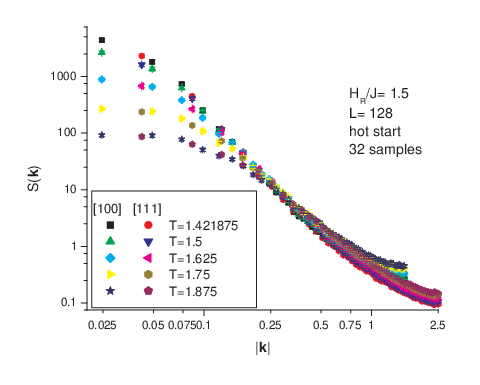

After each sample was relaxed at = 1.421875, a sequence of 6 equilibrated spin states obtained at intervals of 40,960 MCS was Fourier transformed and averaged to calculate . Finally, an average over the 32 samples was performed. Similar procedures were followed at higher values of , where the equilibration times were shorter. The results for along the [1,0,0] and [1,1,1] directions at a sequence of temperatures from down to is shown in Fig. 1. In this range of , for small values of , is increasing as is lowered. At , is virtually independent of for small , indicating that the spin correlations are limited by thermal fluctuations. At , the spin correlations continue to increase as gets smaller, indicating that the spin correlation length is greater than the lattice size. However, the small data for do not fall on a straight line on this log-log plot. We do not know what would happen for larger lattices, but we have no evidence that the data can be explained by a critical point with a correlation length that diverges like some power of temperature.
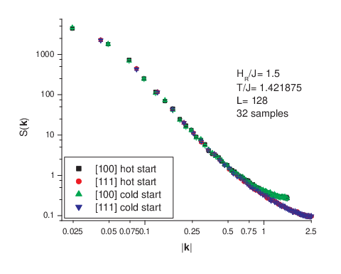
Data were also obtained for the same sets of samples using ordered initial states and warming from = 1.375. At least two, and sometimes more initial ordered states were used for each sample. The initial magnetization directions used were chosen to be close to the direction of the magnetization of the slowly cooled sample with the same set of random fields. This type of initial state was chosen because it was found in the earlier workFis07 that this is the way to find the lowest energy minima in the phase space. The data from the initial condition which gave the lowest average energy for a given sample was then selected for further analysis and comparison with the slowly cooled state data for that sample. The relaxation procedure at for the warmed states was the same one used for the cooled states, and the calculation of proceeded in the same way. In Fig. 2 we compare the for the slowly warmed initial states with the data for the slowly cooled initial states at .
For purposes of comparison with Fig. 2, in Fig. 3 we show data from ref.Fis19, analyzed in the same way. These data for lattices with at are qualitatively similar to the data in Fig. 2. Although is now larger, is smaller. Thermal disorder in Fig. 2 is being replaced by random-field induced disorder in Fig. 3. The resulting change in is not zero, but it is small. The crossover from the large behavior to the small behavior, which happens at , is at a somewhat larger value of in Fig. 3, as predicted by the Imry-Ma argument. Note that the original Imry-Ma argumentIM75 is a zero-temperature argument. One should not assume this idea of thermal disorder replacing random-field induced disorder will work for larger values of , unless and until some evidence of that is found. The small region of Fig. 3 does not appear to be approaching a finite value for in the limit , as discussed in more detail in ref.Fis19.
The reader should note that the estimates of from Fig. 2 and Fig. 3 imply that the lattices studied by Gingras and HuseGH96 are passing through close to , which is the point where Gingras and Huse claim a phase transition occurs at . This coincidence means that their ideas about the nature of the phase transition are not reliable, because their lattices are not large enough to have reached the true small region at their estimated value of the phase transition point.
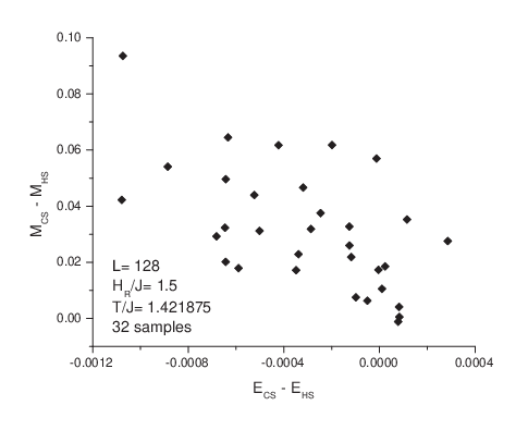
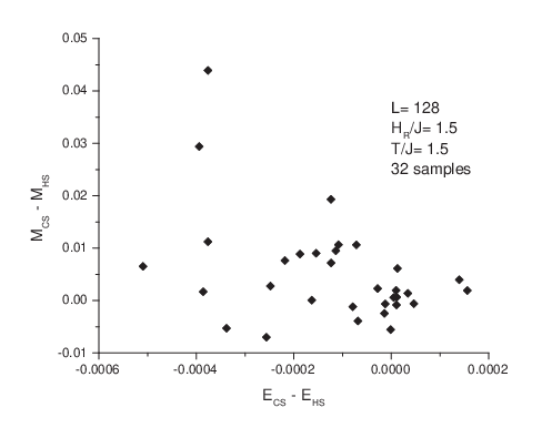
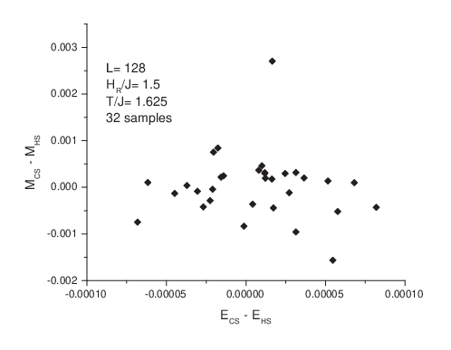
We now return to the discussion of the case. The data for the slowly warmed states and the slowly cooled states at the same value of are indistinguishable for all non-zero values of . However, this is not necessarily true at for a finite sample, as was discussed in detail for the case in ref.Fis19. It is not necessarily true that for a particular sample the spin state is very similar for the warmed state and the cooled state. What actually happens for individual samples is that, in most cases the spin state of the slowly warmed state with an ordered initial condition is significantly different at from the slowly cooled state. However, at the slowly warmed state is, in most cases, essentially indistinguishable from the slowly cooled state. We illustrate this for in Fig. 4, for in Fig. 5 and for in Fig. 6, which plot the differences in the magnetization and the energy for individual samples. Note that in most, but not all samples, at the warmed state has a lower energy and a higher magnetization than the cooled state. At the differences are much smaller, and they no longer have much systematic dependence on the initial conditions.
In Table I we display data for the average magnetization per spin, , the longitudinal magnetic susceptibility per spin, , and the specific heat at zero average field, . It was found for that appears to have a subextensive divergence at ,Fis19 and it is expected that this will also be true at . However, is somewhat longer at . Thus, in order to check how scales with at , we would need data for larger lattices, which is not practical using the computers currently available.
Table I: Thermodynamic data for hot start and cold start initial conditions at = 1.5, for various . (hs) and (cs) mean data obtained using hot start and cold start initial conditions, respectively. The one statistical errors shown are due to the sample-to-sample variations. 1.421875hs 0.0700.008 30.31.2 1.1020.003 1.421875cs 0.1020.008 28.81.1 1.0970.003 1.5hs 0.0510.005 33.91.3 1.2040.004 1.5cs 0.0560.005 33.61.4 1.1200.004 1.625hs 0.0280.003 25.20.5 1.3260.004 1.75hs 0.01420.0012 12.960.36 1.3020.004 1.875hs 0.00810.0006 6.710.22 1.1470.004
There is a peak in centered close to , but it appears to have a finite maximum, as was found for larger values of .Fis19 As should be expected, the peak in increases in height as decreases. Unless there is a phase transition into a ferromagnetic phase, it is not expected that will diverge to infinity for any . There is a very broad peak in centered at about , which is not expected to be associated with long-range correlations. is the temperature where the thermal correlation length is equal to . In the terminology of relaxor ferroelectrics, this is the Burns temperature.BD83
V Discussion
The author thinks it is worth observing that the kind of jumps we are seeing in the energy per spin and the magnetization per spin of finite samples would need to disappear in the limit . The multicritical critical point hypothesis for the behavior of random field models at = 0 says that should be an irrelevant variable at that point. However, the behavior we are seeing along the phase transition line for is not consistent with that hypothesis. If RSB creates a glassy phaseBDD01 between the paramagnet and the ferromagnet when , then this issue is resolved. This is true for both the RFXYM and also the RFIM.
Finding that diverges at low temperatures in the RFXYM as is not surprising. This behavior follows from the results of A. AharonyAha78 for models which have a probability distribution for the random fields which is not isotropic. According to Aharony’s calculation, if this distribution is even slightly anisotropic, then we should see a crossover to RFIM behavior at a sufficiently small value of . We knowImb84; BK87 that in the RFIM is ferromagnetic at low temperature if the random fields are not very strong. The instability to even a small anisotropy in the random field distribution should induce a diverging response in as for the RFXYM in . A similar effect in a related, but somewhat different, model was found by Minchau and Pelcovits.MP85.
More recently, models of quantum-mechanical spins in random fields have been studied at .Car13; AN18 These calculations find logarithmic divergences of the structure factor as in these quantum versions of random field models. It is not clear yet that one should be able to map the classical RFXYM at finite temperature onto a quantum model at = 0. However, A. Aharony’s argument about the instability in the 3D RFXYM makes this connection plausible.
Note that it is only which diverges for the 3D RFXYM. Unlike the situation for the Kosterlitz-Thouless transition, we are not seeing any divergence of . The difference in the behavior of and is due to the fact that the local magnetization, , has a non-zero average value even at high in a random field model. What is going on here is that the terms in Eqn. 4 are canceling against the terms, and giving a finite net result, even at . It is very unclear that the behavior we are seeing can be attributed to topological defects. However, the range of uncertainty in is significant, and we cannot rule out that the RSB phase transition occurs at the same temperature as the percolation transition of the vortex lines on the dual lattice, as proposed by Gingras and Huse.GH96
Several years ago, calculations of Chudnovsky and coworkersGCP13; PGC14 made much stronger claims. These authors use a downhill relaxation algorithm for the 3D RFXYM at . The states found by their algorithm are local energy minima of the Hamiltonian which have values of of approximately 0.80. We see no reason to believe that such a downhill relaxation algorithm should be able to come anywhere close to finding the true ground state of a sample for large at . It is the current author’s opinion that in order for the results of such a downhill relaxation algorithm to be convincing, they must be done using an which is a power of 2. In that case, could be calculated in the same way it has been done here. A properly relaxed state for a ferromagnetic state of an model must have a divergent peak of for .
The results we are finding at are qualitatively similar to the results we found previouslyFis19 at . Chudnovsky et al. say that they find no ground state magnetization near . We consider an abrupt qualitative change in the ground state behavior between and , as claimed by Chudnovsky et al., to be implausible for this model. Since our Monte Carlo calculations are limited to , we cannot obtain results in the regime where the thermal correlation length is larger than when . There has been no attempt in this work to equilibrate samples at temperatures below . Therefore, we have no data which directly address the question of whether the RFXYM shows true ferromagnetism in . We do not claim that we know what happens for small values of .
It appears to the author that what is going on in this model is a broken ergodicity transition in the phase space, without any change in the spatial symmetry. In that sense, it is similar to a spin-glass phase transition. However, a random field model does not have the two-fold Kramers degeneracy of a spin glass. Therefore the broken ergodicity occurs in the random field model in a purer form, without the extra complication of the two-fold symmetry in the phase space.
The reader may be tempted to object that such a phase transition cannot be described within the usual formalism of equilibrium statistical mechanics, based on the canonical partition function
| (7) |
where is given in Eqn. 1. We are thinking now about a particular sample, so the variables are fixed. For a classical system, the standard formulas based on do not have any dependence on dynamics. That is the point. The fact that our Monte Carlo calculation sees that the hot start states and the cold start states we find for are not the same means that these results cannot be described by . Our calculation is not finding the partition function. When the dynamical relaxation time is infinite over a range of , will not give us the behavior seen in a laboratory experiment. Of course, strictly speaking, the relaxation time is not actually infinite in a finite sample. However, real experiments are done on finite samples, in finite times.
The idea of the broken ergodicity transition is exactly that we need to include dynamics in order to understand what is going on. It is true that if we ran the Monte Carlo calculation for any finite lattice a very long time, the results would, in principle, eventually converge to the for that particular finite lattice. However, there is an order of limits issue. A broken ergodicity transition, like all thermodynamic phase transitions, only exists in the limit of an infinite system. To get correct results in the thermodynamic limit, we need to take the limit in an appropriate way. We should not take the limit of infinite time while holding fixed. The results which come from a Monte Carlo calculation may be thought of as telling us that the RSB in the RFXYM is happening in three space dimensions and one time dimension at some , if is not too large. This is completely independent of whether or not there might be a ferromagnetic transition at some lower temperature. A helpful review of Monte Carlo calculations, which discusses critical slowing down of the dynamical behavior at a phase transition, has been given by Sokal.Sok92 One could say that, for the RFXYM problem, dynamical slowing down is not a bug, it is a feature.
Hui and BerkerHB89 argued that the vanishing of the latent heat implied that a critical fixed point should exist. This author does not see, however, why such a fixed point, with its associated divergent correlation length, should generally exist in a model which has no translation symmetry, except in those cases where the randomness is an irrelevant operator.Har74 It is certainly true that there are some cases where such fixed points have been found using -expansion calculations. Subextensive singularitiesFis19 in the specific heat and the magnetization are completely consistent with the Aizenman-Wehr Theorem.AW89; AW90
VI Summary
In this work we have performed Monte Carlo studies of the 3D RFXYM on simple cubic lattices, with a random field strength of . We compared the properties of slowly cooled states and slowly heated states at , and . The temperature at which there appears to be a phase transition described by a divergence in the structure factor at is probably between and . The behavior is qualitatively the same as what was found earlierFis19 for somewhat larger values of . We have also computed values of the magnetic susceptibility and the specific heat. The data are consistent with the idea that in the RFXYM has a phase transition into a phase described by broken ergodicity, as long as the strength of is not too large. We do not believe that there is a ferromagnetic phase at any value of for . These results appear to be related to RSBBDD01, and to recent work on quantum disorder.AN18
Acknowledgements.
The author thanks N. Sourlas for a helpful conversation about the recent work on the random field Ising model, and Ofer Aharony for a discussion of his recent results on quantum disordered models. This work used the Extreme Science and Engineering Discovery Environment (XSEDE) Bridges Regular Memory at the Pittsburgh Supercomputer Center through allocations DMR170067 and DMR180003. The author thanks the staff of the PSC for their help.References
- (1) A. I. Larkin, Zh. Eksp. Teor. Fiz. 58, 1466 (1970) [Sov. Phys. JETP 31, 784 (1970)].
- (2) Y. Imry and S.-K. Ma, Phys. Rev. Lett. 35, 1399 (1975).
- (3) A. Aharony, Y. Imry and S.-K. Ma, Phys. Rev. Lett. 37, 1364 (1976).
- (4) M. Mezard and A. P. Young, Europhys. Lett. 18, 653 (1992).
- (5) E. Brezin and C. De Dominicis, Eur. Phys. J. B 19. 467 (2001).
- (6) M. J. P. Gingras and D. A. Huse, Phys. Rev. B 53, 15193 (1996).
- (7) R. Fisch, Phys. Rev. B 55, 8211 (1997).
- (8) R. Fisch, Phys. Rev. B 76, 214435 (2007).
- (9) R. Fisch, arXiv:1001.3397.
- (10) M. Aizenman and J. Wehr, Phys. Rev. Lett. 62, 2503 (1989); erratum: Phys. Rev. Lett. 64, 1311 (1990).
- (11) M. Aizenman and J. Wehr, Commun. Math. Phys. 130, 489 (1990).
- (12) R. Fisch, arXiv:1812,09318v2.
- (13) D. A. Garanin, E. M. Chudnovsky and T. Proctor, Phys. Rev. B 88, 224418 (2013).
- (14) J. Z. Imbrie, Phys. Rev. Lett. 53, 1747 (1984).
- (15) J. Bricmont and A. Kupiainen, Phys. Rev. Lett. 59, 1829 (1987).
- (16) N. G. Fytas, V. Martin-Mayor, M. Picco and N. Sourlas, J. Stat.Mech. 033302 (2017).
- (17) N. G. Fytas, V. Martin-Mayor, M. Picco and N. Sourlas, Phys. Rev. E 95, 042117 (2017).
- (18) N. G. Fytas, V. Martin-Mayor, M. Picco and N. Sourlas, J. Stat. Phys. 172, 665 (2018).
- (19) T. C. Proctor, D. A. Garanin and E. M. Chudnovsky, Phys. Rev. Lett. 112, 097201 (2014).
- (20) M. Tissier and G. Tarjus, Phys. Rev. Lett. 96, 087202 (2006); Phys. Rev B 74, 214419 (2006).
- (21) P. Le Doussal and K. J. Wiese, Phys. Rev. Lett. 96, 197202 (2006).
- (22) M. Tissier and G. Tarjus, Phys. Rev B 78, 024204 (2008).
- (23) J. V. Jose, L. P. Kadanoff, S. Kirkpatrick and D. R. Nelson, Phys. Rev. B 16, 1217 (1977).
- (24) A. Houghton, R. D. Kenway and S. C. Ying, Phys. Rev. B 23, 298 (1981).
- (25) J. L. Cardy and S. Ostlund, Phys. Rev. B 25, 6899 (1982).
- (26) K. G. Wilson and J. Kogut, Phys. Rprt. 12, 75 (1974).
- (27) R. Fisch, Phys. Rev. B 46, 242 (1992).
- (28) W. Janke, Phys. Lett. A 148, 306 (1990).
- (29) N. Sourlas, J. Stat. Phys. 172, 673 (2018).
- (30) G. Burns and F. H. Dacol, Phys. Rev. B 28, 2527 (1983).
- (31) A. Aharony, Phys. Rev. B 18, 3328 (1978).
- (32) B. J. Minchau and R. A. Pelcovits, Phys. Rev. B 32, 3081 (1985).
- (33) J. Cardy, J. Phys. A 46, 494001 (2013).
- (34) O. Aharony and V. Narovlansky, Phys. Rev. D 98, 045012 (2018).
- (35) A. D. Sokal, in ”Quantum Fields on the Computer”, M. Creutz, ed., (World Scientific, Singapore, 1992), p.p. 211-274.
- (36) K. Hui and A. N. Berker, Phys. Rev. Lett. 62, 2507 (1989).
- (37) A. B. Harris, J. Phys. C 7, 1671 (1974).