Sampling for Bayesian Mixture Models: MCMC with Polynomial-Time Mixing

Wenlong Mou^⋄

Nhat Ho^⋄

Martin J. Wainwright^⋄,†,‡

Peter L. Bartlett^⋄,†

Michael I. Jordan^⋄,†

Department of Electrical Engineering and Computer Sciences^⋄

Department of Statistics^†

UC Berkeley

Voleon Group, Berkeley^‡

August 11, 2026

Abstract

We study the problem of sampling from the power posterior distribution in Bayesian Gaussian mixture models, a robust version of the classical posterior. This power posterior is known to be non-log-concave and multi-modal, which leads to exponential mixing times for some standard MCMC algorithms. We introduce and study the Reflected Metropolis-Hastings Random Walk (RMRW) algorithm for sampling. For symmetric two-component Gaussian mixtures, we prove that its mixing time is bounded as $d^{1.5}(d+\|\theta_{0}\|^{2})^{4.5}$ as long as the sample size $n$ is of the order $d(d+\|\theta_{0}\|^{2})$ . Notably, this result requires no conditions on the separation of the two means. En route to proving this bound, we establish some new results of possible independent interest that allow for combining Poincaré inequalities for conditional and marginal densities.

1 Introduction

Bayesian mixture models are a popular class of models, frequently used for the purposes of density estimation (e.g., [18, 19, 20]). Various researchers have studied posterior inference of parameters in Bayesian mixture models [24, 42, 23], so that the statistical behavior of such models is relatively well-understood. In contrast, much less is known about the efficiency of different algorithms for sampling from the posterior distributions that arise from Bayesian mixture models. A standard approach for doing so is via some form of Markov Chain Monte Carlo (MCMC). Many different types of MCMC algorithms have been introduced for various types of Bayesian mixture models, including finite Bayesian mixture models [21, 49, 50, 26, 40], Dirichlet process mixture models [37, 41, 25, 28], and hierarchical and nested Dirichlet process models [52, 47]. Despite the plethora of possible MCMC methods, upper bounds on their mixing times are often challenging to establish. We refer the reader to the papers [27, 3, 55, 48, 57] for non-asymptotic upper bounds on mixing times for certain types of Bayesian models, different from those studied in this paper.

In recent years, it has been increasingly common in the Bayesian literature to make use of a fractional likelihood—meaning an ordinary likelihood raised to some fractional power. Combining such a fractional likelihood with a prior distribution in the usual way leads to a class of posteriors known as power posterior or fractional posterior distributions. The power posterior distributions have been shown to have attractive properties in terms of robustness to mis-specification in Bayesian mixture models [39], and have been used in various applications (e.g., [51, 2]). Some theoretical recent work by Yang et al. [4] provides contraction rates for a range of power posteriors.

At the same time, there is now a substantial and evolving line of work on algorithms for sampling from continuous distributions that are based on discretizations of SDEs such as the Langevin diffusion [46]. Such algorithms are now relatively well-understood when the target distribution is log-concave, with many provably efficient algorithms proposed (e.g., see the papers [15, 13, 32, 38, 14] and references therein). The efficiency of sampling from log-concave densities stems from their favorable isoperimetric properties [5], which ensure that the continuous-time Langevin diffusion mixes very fast. By way of contrast, sampling from multi-modal distributions is known to be hard in the worst case. There are multi-modal densities for which even the continuous-time diffusion can take exponential time in order to escape from a basin of attraction [7]. However, these results are worst case in nature, and so do not preclude the existence of efficient algorithms for particular multi-modal densities, such as those arising from Bayesian mixture models.

Recently, a number of researchers have tackled the algorithmic challenge of sampling from multi-modal distributions. For target distributions that satisfy a distant dissipativity condition, it is possible to prove global convergence, with the rate depending on quantities such as the spectral gap, log-Sobolev constant or Stein factor [44, 16]. These quantities typically lead to a mixing time that grows exponentially in the problem parameters. When the potential function is strongly convex outside a ball and non-convex inside this ball, there are bounds on the mixing time of the Langevin and Hamiltonian Monte Carlo algorithms [12, 36, 6]. For this class of algorithms, the time complexity is typically exponential in the product $LR^{2}$ , where $L$ is a smoothness parameter and $R$ is the radius of that ball.

If we consider such results in the context of power posterior distributions in Bayesian mixtures, the radius $R$ is potentially large and dimension-dependent. For instance, for a symmetric two-component mixture model, with means at $\theta_{0}$ and $-\theta_{0}$ , the radius $R$ scales proportionally with $\|\theta_{0}\|_{2}$ , a measure of the separation between the components. Thus, a curious phenomenon arises: although stronger separation between the components makes the estimation problem easier, it makes the sampling problem more difficult (at least in terms of the best known upper bounds). Indeed, some past work [9] shown that the complexity of sampling from these posteriors can grow exponentially for certain algorithms.

A line of recent work [31, 17] has attacked the multi-modal sampling problem by simulated tempering. In particular, these authors studied gradient-based algorithms for sampling from mixture of homogeneous strongly-log-concave distributions. Sampling from such distributions can be directly solved by log-concave sampling methods; therefore, difficulties in the simulated tempering approach mainly arise from the restriction to gradient oracles. For power posterior sampling in mixture models, even if oracle access is not restricted to gradients and the structure of the landscape is known, difficulties still persist.

1.1 Contributions

The main contribution of this paper is to propose a particular algorithm for sampling in a class of Bayesian mixture models, and to prove that it has mixing time bounded by a polynomial function of dimension and other problem parameters. More specifically, we consider a power posterior distribution of the form

\displaystyle\Pi_{n,\beta/n}\Big(\theta\mid\{X_{i}\}_{i=1}^{n}\Big)

\displaystyle\;\propto\;\;\prod\limits_{i=1}^{n}\left(f_{\theta}(X_{i})\right)^{\beta/n}\lambda(\theta),

(1)

where $\beta\in(0,n)$ is the power parameter; $\lambda$ is a prior over $\theta$ ; $f_{\theta_{0}}(x):=\frac{1}{2}\varphi(x;\theta_{0},I_{d})+\frac{1}{2}\varphi(x;-\theta_{0},I_{d})$ is the density of a two-component Gaussian mixture model in ^d. The class of power posterior distributions is a generalization of the usual posterior, to which it reduces when $\beta=n$ .

Of course, the posterior is a random object, since the observed data $\{X_{i}\}_{i=1}^{n}$ have been drawn randomly from the mixture distribution. Our main contributions are to prove certain high probability guarantees on the behavior of an algorithm for drawing samples from the posterior, where the probability is taken over the randomness of the observed data.

•

We develop an MCMC algorithm, referred to as the Reflected Metropolis-Hastings Random Walk (RMRW) algorithm, for drawing samples from posterior distributions of the form (1). We prove that with high probability over the randomness of the samples, this algorithm has polynomial mixing time—in particular, running it for $\mathrm{poly}(d,\|\theta_{0}\|,\log\frac{1}{\varepsilon})$ steps yields a sample from a distribution that is $\varepsilon$ -close to the correct posterior distribution in total variation (TV) distance, as long as the number of samples satisfies $n\gtrsim d^{2}+\beta^{2}d$ . The result does not require any separation between the components of the mixture distribution. Furthermore, we demonstrate that RMRW algorithm also achieves polynomial mixing time under model mis-specification.
•

Despite the seemingly simplicity of the symmetric Gaussian mixtures, the sampling problems associated with their power posterior are challenging. In particular, the population and empirical log-likelihoods for the symmetric Gaussian mixtures have two basins of attraction [1], which are symmetric. There is a potentially high cost for moving across the saddle point. In order to avoid such high cost, we allow the RMRW algorithm to jump between components directly.
•

For the population landscape, fast mixing within each partition requires an isoperimetric inequality. A technical challenge arises in establishing this inequality: despite the unimodality of each basin of attraction, they are only quasi-concave, and such distributions are known to have poor isoperimetry in the worst case [10]. Moreover, there can be a non-trivial proportion of mass assigned to the neighborhood of the saddle point. For this reason, the Markov chain has to explore the part with negative curvature in a careful way, instead of entirely avoiding it by a suitably large initialization [56]. Addressing these properties requires a careful analysis of the geometry of symmetric Gaussian mixtures. In particular, the population log-likelihood of these models is quasi-convex in the direction of $\theta_{0}$ restricted to a partition, and convex in all other directions. In order to show isoperimetry for this function and guarantee good isoperimetry within each partition, we establish general structural results that combine the Poincaré inequalities for conditional and marginal densities. Combining these results leads to the polynomial-time mixing rate guarantee for the RMRW algorithm.

We note in passing that our novel Poincaré inequality, while applied here only to Gaussian mixtures, is of potential use for a much broader class of non-log-concave densities. Our isoperimetric inequalities are based only on geometric properties, so can hold for distributions that need not be log-concave. The bounds from past work on sampling from mixture distribution [31, 17] are based directly on the isoperimetric constants for each mixture component, and so require each mixture component to be well-behaved.

By contrast, the isoperimetric inequalities proved in this paper are linked directly to the geometric structure of the target density. For this reason, we suspect that our results may be useful for analyzing sampling algorithms for more general classes of distributions. Finally, our proof follows the avenue of relating the sample log-likelihood to the population log-likelihood via empirical process theory, and then exploiting the structure of the population problem. This proof technique is also applicable to sampling problems from other types of Bayesian posterior distributions.

In the existing literature, many results have been established to derive log-Sobolev inequalities by combining those for marginals and conditionals [43, 33, 22]. Such results play a key role in understanding the dynamics of certain statistical physics systems. Our technical lemma for combining the Poincaré inequalities can be seen as parallel to this existing literature. In our setup, it is also important that only the Poincaré inequalities are assumed for the marginal and conditional distributions; indeed, the joint distribution is not strongly-log-concave and may not satisfy log-Sobolev inequality with a good constant.

1.2 Organization and notation

The remainder of the paper is organized as follows. In Section 2, we provide the setup for symmetric Gaussian mixtures and several useful definitions for establishing mixing time of MCMC algorithms. In Section 3, we describe the RMRW algorithm including some of the underlying geometry, and sketch out our analysis of its mixing time. Several key results with the isoperimetric inequalities and conductance of Markov chain defined by RMRW algorithm are presented in Section 4 and Section 5. The proofs for key results in the paper are in Section 6 whereas the proofs for remaining results are deferred to the appendices. We conclude with a discussion in Section 7.

Notation and basic definitions.

For each positive integer $n$ , we use $[n]$ to denote the set $\{1,2,\ldots,n\}$ . For any set $A$ , we denote $A^{c}$ as its complement. For any vector $x\in\mathbb{R}^{d}$ , we denote $x_{i}$ as its $i$ -th component while $x_{-i}$ stands for all the components except $i$ -th component for $i=1,\ldots,d$ . The expression $a_{n}\succsim b_{n}$ will be used to denote $a_{n}\geq cb_{n}$ for some positive universal constant $c$ . Given two density functions $p$ and $q$ with respect to Lebesgue measure $\mu$ , the squared Hellinger distance between $p$ and $q$ is given by $h^{2}(p,q)=\frac{1}{2}\int(\sqrt{p(x)}-\sqrt{q(x)})^{2}d\mu(x)$ . The total variation (TV) distance and Kullback-Leibler (KL) divergence are given by

\displaystyle d_{\mbox{\tiny{TV}}}(p,q)=\frac{1}{2}\int\left|p(x)-q(x)\right|d\mu(x),\quad\mbox{and}\quad\text{KL}(p,q)=\int\log(p(x)/q(x))p(x)d\mu(x),

respectively. A function $f:\mathbb{R}^{d}\to\mathbb{R}$ is quasi-convex if for any $\alpha\in\mathbb{R}$ , the level set $\{x\in\real^{d}\,\mid\,f(x)\leq\alpha\}$ is a convex set.

2 Problem set-up

In this paper, we study mixing time for the Bayesian posterior distributions that are induced by a symmetric two-component location Gaussian mixture model, or in short, a symmetric Gaussian mixture. An instance of such a mixture model is characterized by a density of the form

\displaystyle f_{\theta_{0}}(x)

\displaystyle:=\frac{1}{2}\varphi(x;\theta_{0},I_{d})+\frac{1}{2}\varphi(x;-\theta_{0},I_{d}).

(2)

Here $\varphi(\>\cdot\>;\theta,I_{d})$ denotes the multivariate Gaussian distribution with location parameter $\theta\in\mathbb{R}^{d}$ and covariance matrix $I_{d}$ . We are interested in the problem of sampling from the power posterior distribution induced by a symmetric Gaussian mixture and a prior $\lambda$ . It takes the form

\displaystyle\Pi_{n,\beta/n}\Big(\theta\mid\{X_{i}\}_{i=1}^{n}\Big):=\dfrac{\prod\limits_{i=1}^{n}\left(f_{\theta}(X_{i})\right)^{\beta/n}\lambda(\theta)}{{\displaystyle\int\prod\limits_{i=1}^{n}\left(f_{u}(X_{i})\right)^{\beta/n}\lambda(u)du}},

(3)

where $\beta\in(0,n)$ is a parameter. While the setting of $\beta$ typically varies as a function of the sample size $n$ , here we omit this dependence so as to simplify notation. The exponentiated likelihood in the numerator (disregarding the prior term) is often referred to as the power likelihood.

Note that sampling from the distribution (3) is equivalent to sampling from the distribution with density $\pi$ proportional to $e^{-U(\theta)}$ , where

\displaystyle U(\theta):=\frac{\beta}{n}\sum_{i=1}^{n}\log\left(\frac{1}{2}\varphi(\theta-X_{i})+\frac{1}{2}\varphi(\theta+X_{i})\right)+\log\lambda(\theta).

(4)

For the symmetric Gaussian mixtures, the power posterior distribution is non-log-concave and multi-modal. In such context, there are few polynomial-time guarantees on sampling algorithms. Most existing works on sampling from multi-modal distributions require the function $-\log\pi$ to be convex outside a ball, and have exponential dependence on the radius of this ball [12, 36, 6]. When applying these results to power posterior sampling in symmetric Gaussian mixtures, the radius of this ball scales with separation between mixture components, i.e., $\|\theta_{0}\|$ . From this fact arises a curious phenomenon: while larger separations between mixture components makes estimation easier, it appears to make sampling harder, at least in terms of known upper bounds.

Note that the power posterior (3) is a random measure, since it depends on the observations $\{X_{i}\}_{i=1}^{n}$ . For the purposes of analysis, it turns out to be convenient to introduce a deterministic measure that we refer to as the population power posterior. In particular, given the symmetric Gaussian mixture (2), the population power posterior is defined by a density of the form $\pi_{0}(\theta)\propto e^{-U_{0}(\theta)}$ , where

\displaystyle U_{0}(\theta):=\beta\cdot{\mathbb{E}}\log\left(\frac{1}{2}\varphi(\theta-X)+\frac{1}{2}\varphi(\theta+X)\right)+\log\lambda(\theta).

Here the expectation is taken over a random observation $X\sim\frac{1}{2}\mathcal{N}(\theta_{0},I_{d})+\frac{1}{2}\mathcal{N}(-\theta_{0},I_{d})$ taken from the underlying two-component Gaussian mixture.

3 Polynomial time MCMC algorithm

With these definitions in hand, we are now ready to describe our MCMC algorithm for sampling from the power posterior (3). For reasons to become clear, we refer to it as the Reflected Metropolis-Hastings Random Walk (RMRW) algorithm. We first describe that algorithm based on population power posterior sampling and state a formal result with its polynomial mixing time in Section 3.1. We then provide geometric intuition behind the polynomial mixing time of RMRW algorithm, along with a sketch that outlines some key ideas in the proof.

3.1 Reflected Metropolis-Hastings Random Walk algorithm

The RMRW algorithm we develop in this section relies on the special structure of symmetric Gaussian mixtures. In pseudocode, it takes the following form:

0: Oracle access to potential function

F

, step size

\eta>0

0: Approximate sample

\theta\sim\pi\propto e^{-F}

Sample

\theta^{(0)}\sim\mathcal{N}(0,I_{d})

for

t=1,2,\cdots

Let

Y\sim\theta^{(t-1)}+\sqrt{\eta}\mathcal{N}(0,I_{d})

Let

Z=Y

with probability

\frac{1}{2}

and

Z=-Y

with probability

\frac{1}{2}

Let

\theta^{(t)}=\begin{cases}Z&\text{with probability }\min\left(1,\exp(F(Z)-F(\theta^{(t-1)}))\right)\\ \theta^{(t-1)}&\text{otherwise}\end{cases}.

end for

Algorithm 1 Reflected Metropolis-Hastings Random Walk Algorithm

As seen from this pseudocode, the RMRW algorithm is a random walk, based on an isotropic Gaussian proposal distribution, combined with a reflection through origin, along with a final adjustment using a Metropolis-Hastings correction. Note that the algorithm does not exploit any information about the gradient of the potential function, and so can be seen as a zero^th-order procedure (meaning that it only uses the value of the potential function as opposed to its gradient).

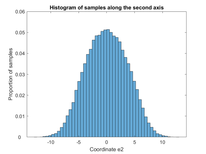
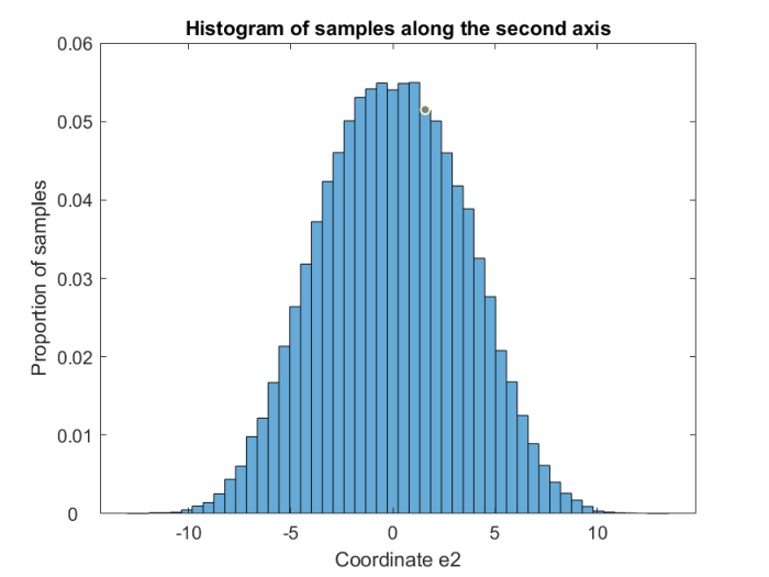
We also demonstrate the shape of the power posterior distribution by simulation results based on our RMRW algorithm. We consider $n=100$ data points generated from a $10$ -dimensional symmetric two-component Gaussian mixture model (2) with $\theta_{0}=ae_{1}$ for $a\in\{0,5\}$ and $e_{1}=(1,0,\ldots,0)$ . The fraction parameter $\beta$ is chosen as $\beta=8$ . We generate the samples by taking $100000$ consecutive iterates of the RMRW algorithm. In Figure 1, we show the histograms for the projection of samples drawn from the RMRW algorithm onto the first and second dimension.

Refer to caption — Figure 1: Illustration of samples from RMRW algorithm for approximating power posterior of a $10$ -dimensional symmetric two-component Gaussian mixture model based on $100$ data points, with $\beta=8$ . (a), (b): Case $a=5$ for which the components are well-separated. Panel (a) shows projection of samples onto $e_{1}$ , the direction of the true parameter $\theta_{0}$ , whereas plot (b) shows the projection of the samples onto $e_{2}$ , which is orthogonal to the true parameter. Due to the separation, the projection in the direction $e_{1}$ exhibits bimodality. (c), (d). Same plots with $a=0$ , for which there is no separation between components. Notice the biomodality has now disappeared.

3.2 Bound on mixing time and geometric intuition

It is straightforward to show that the target distribution is a stationary distribution of Markov chain defined by Algorithm 1. Of interest to us is a bound on the mixing time of the algorithm, defined as

\displaystyle T(\epsilon)

\displaystyle:=\inf_{t=1,2,\ldots}\left\{d_{TV}(\pi^{t},\pi)\leq\epsilon\right\},

(5)

where $\pi^{t}$ denotes the distribution of the algorithm’s iterates at time $t$ . In this paper, we study the case of a uniform and hence improper prior—namely, the choice $\lambda(\theta)=1$ for all $\theta\in\real^{d}$ . This improper prior can be viewed as the limiting case of the normal prior $\mathcal{N}(0,\sigma^{2}I_{d})$ as $\sigma\to\infty$ . We note also that the techniques in the paper can be extended to the case when $\lambda(\theta)$ is a Gaussian density function of the form $\mathcal{N}(0,\sigma^{2}I_{d})$ for $\sigma>0$ , but we refrain from doing so in order to simplify the statement. In the following statement, we use $C_{1}$ and $C_{2}$ to denote universal positive constants.

Theorem 1 (Mixing time of RMRW algorithm).

Let $\varepsilon\in(0,1)$ be a target TV distance error, and let $\delta\in(0,1)$ be a pre-specified failure probability. Suppose that the sample size $n$ is lower bounded as $n\geq C_{1}d\left(\beta^{2}(1+\|\theta_{0}\|^{2})+d\right)\log(d(\|\theta_{0}\|+1)/\delta)$ , and the RMRW algorithm is run with the (random) potential function $U$ in equation (4). Then with probability at least $1-\delta$ over this randomness, the mixing time is bounded as

\displaystyle T(\epsilon)

\displaystyle\leq C_{2}\;d^{3/2}\;\left(d+\|\theta_{0}\|^{2}\right)^{9/2}\log^{11/2}\left(\frac{1}{\varepsilon}\right).

In order to provide intuition for the result in Theorem 1, we sketch out the main steps of the proof in Section 3.4; see Section 6.2.3 for the full proof with all technical details.

3.3 Geometric intuition

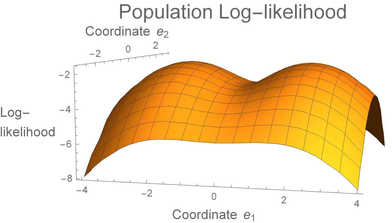
Figure 2 provides some geometric intuition for the algorithm, and its relatively fast mixing. Panel (a) provides a surface plot of the negative log-likelihood at population level for a problem in $d=2$ dimensions. Note that the negative log-likelihood is symmetric around the origin and has global minima at $\theta_{0}$ and $-\theta_{0}$ . In any direction orthogonal to $\theta_{0}$ , the negative log-likelihood is a convex function. The $\theta_{0}$ direction is the interesting one: in this direction, the landscape can be partitioned into two symmetric components; within each of them, the negative log-likelihood is quasi-convex. We exploit these properties in order to bound the conductance of Markov chain in RMRW algorithm.

An additional challenge is the existence of a saddle point at $\theta=0$ . In the context of computing point estimates for mixture models, this difficulty can be side-stepped by initializing an iterative algorithm with any vector of sufficiently large norm [56]. The sampling problem—in contrast to the problem of point estimation—requires a complete exploration of the probability surface, and the mass with negative curvature cannot be ignored. Accordingly, the following sections are devoted to the development of some new tools for establishing Poincaré and isoperimetric inequalities over a partition. We would like to note that though several geometric conditions can be verified analytically for the population power posterior, the calculations are delicate and do not generalize to the empirical counterpart. Fortunately, by the Holley-Stroock principle, conductance results are robust with multiplicative perturbation of the density. As a consequence, we can use empirical process theory to guarantee global uniform convergence of the potential function. This control allows us to transfer conductance bounds from the population to the empirical power posterior.

3.4 Proof sketch

In this section, we provide a sketch of the proof of Theorem 1. The argument makes use of the standard notions of a Poincaré inequality, and the $s$ -conductance [34], which we now define.

Poincaré inequality:

Given a set $\Omega\subseteq\mathbb{R}^{d}$ with smooth boundary, consider a probability distribution $\pi$ supported on $\Omega$ . It is said to satisfy the Poincaré inequality with constant $C>0$ if the inequality

\displaystyle\int_{\Omega}f^{2}(x)d\pi(x)\leq C\int_{\Omega}\|\nabla f(x)\|^{2}d\pi(x)

holds for all functions $f$ in the Sobolev space $H^{1}(\pi,\Omega)$ such that ${\mathbb{E}}_{\pi}f(X)=0$ .

$s$ -conductance:

For a space $\Omega$ accompanied with a $\sigma$ -algebra $\mathcal{F}$ , we consider a discrete-time Markov chain with transition kernel $\mathcal{T}_{x}(S):\Omega\times\mathcal{F}\rightarrow\mathbb{R}$ whose stationary distribution is $\pi$ . For any $s>0$ , the $s$ -conductance of this Markov chain is

\displaystyle\Phi_{s}(\pi):=\inf_{S\in\mathcal{F}:s<\pi(S)\leq\frac{1}{2}}\frac{\int T_{x}(S^{c})d\pi(x)}{\pi(S)-s}.

(6)

With these definitions in hand, we now sketch out the proof, which consists of three main steps:

Step 1:

First, since the two basins of attraction in the population log-likelihood are symmetric, we can partition the space into two symmetric components along direction $\theta_{0}$ , and analyze the isoperimetry within each of them. Even within a partition, the density is neither log-concave nor $s$ -concave, making existing isoperimetric bounds inapplicable. However, a key geometric observation is that the marginal density at $\theta_{0}$ direction is quasi-concave, and the conditional density for other directions are log-concave. We derive a novel result for combining Poincaré inequalities of these densities (Lemma 1 in Section 4.1), and use it to obtain the following isoperimetric result:

Theorem 2.

For any positive constants $A>\max(\|\theta_{0}\|,1)$ and $M>1$ , the Cheeger constant $\zeta$ for density $\pi_{0}$ restricted to $[0,A]\times\mathcal{B}(0,M)$ is lower bounded as

\displaystyle\zeta\geq\frac{c}{A^{5}M^{2}}\;\frac{1}{\sqrt{d}}.

(7)

In the lower bound (7), the constant $c>0$ is independent of $A$ and $M$ . The key results that underlie this theorem are given in Sections 4.1 and 4.2, whereas the technical details of the proof are given in Section 6.1.3.

Step 2:

The second step is to establish conductance results for the Markov chain defined by RMRW algorithm. Theorem 2 provides a lower bound on the Cheeger constants inside each partition, which implies the fast mixing of the Metropolized random walk within each component. In order to make the Markov chain mix fast in the whole space without waiting for the exponential exit time of a basin-of-attraction, we allow it to jump between two components. Due to the symmetry of population log-likelihood, this leads to $s$ -conductance lower bound on the Markov chain defined by RMRW algorithm with density $\pi_{0}\propto e^{-U_{0}}$ as follows:

\displaystyle\Phi_{s}(\pi_{0})

\displaystyle\gtrsim\;d^{-1/4}\Big\{\sqrt{d}+\|\theta_{0}\|+\sqrt{\log(1/s)}\Big\}^{-9/2}.

(8)

Section 5.1 provides various results that lead to this conductance bound.

Step 3:

Our final step is to translate results for population power posterior to its empirical counterpart, in particular using techniques from empirical process theory. Lemma 4 provides control on the deviations between the empirical and population posteriors, up to a multiplicative factor. Since the $s$ -conductance is robust with respect to such multiplicative perturbations, this control allows us to translate bounds on the mixing rate of a chain on the population posterior to the actual Markov chain that evolves according to the empirical power posterior.

4 Geometric results and isoperimetry

This section is dedicated to the proof of Theorem 2. We first provide general structural results about Poincaré inequalities for certain classes of non-log-concave densities. We then validate the assumptions in the case of population power posterior for the symmetric two-component Gaussian mixture models (2). Lemma 1 for combining Poincaré inequalities for conditional and marginal densities is of possible independent interest.

4.1 General structural results

We establish structural lemmas that are needed to prove the isoperimetric inequalities for the population power posterior. The potential function $U_{0}$ is convex in all directions that are orthogonal to $\theta_{0}$ . In contrast, it is non-convex in the direction $\theta_{0}$ , and so a special treatment is required. In particular, we make use of the following lemma, which allows us to combine Poincaré inequalities for conditional and marginal densities together so as to obtain the Poincaré inequality for the whole density.

Lemma 1.

Consider a probability measure $\pi$ that is continuously differentiable over its support $\Omega_{1}\times\Omega_{2}$ , where $\Omega_{1}\subseteq\mathbb{R}^{d_{1}}$ and $\Omega_{2}\subseteq\mathbb{R}^{d_{2}}$ are closed sets. For $X=(X_{1},X_{2})\sim\pi$ , suppose that

•

The marginal distribution of $X_{1}$ satisfies a Poincaré inequality with constant $C_{1}$ .
•

For any $x_{1}\in\Omega_{1}$ , the conditional distribution $X_{2}|X_{1}=x_{1}$ satisfies a Poincaré inequality with constant $C_{2}$ uniform in $x_{1}$ .
•

The function $x_{1}\mapsto\log\pi(x_{2}|x_{1})$ is uniformly differentiable, and moreover, there exists a constant $L>0$ such that $\sup\limits_{x_{1}\in\Omega_{1},x_{2}\in\Omega_{2}}\left\|\nabla_{x_{1}}\log\pi(x_{2}|x_{1})\right\|_{2}\leq L$ .

Under these conditions, the density $\pi$ satisfies a Poincaré inequality with the constant

\displaystyle\tilde{C}=2\left(C_{1}+C_{2}+C_{1}C_{2}L^{2}\right).

See Section 6.1.1 for the proof of this claim.

Let us sketch the main ideas underlying this lemma. For any zero-mean function $h$ on $\Omega_{1}\times\Omega_{2}$ , we need to control the variance of $h(X_{1},X_{2})$ using the second moment of its gradient. For any $x_{1}\in\Omega_{1}$ fixed, we perform bias-variance decomposition on $h^{2}(x_{1},X_{2})$ with $X_{2}\sim\pi(x_{2}|x_{1})$ . The variance term can be easily dealt with by the Poincaré inequality for the conditional density. For the bias term ${\mathbb{E}}_{\pi}\left(h(X_{1},X_{2})|X_{1}=x_{1}\right)$ , since its expectation is 0, we can still control its second moment using its gradient based on the Poincaré inequality for marginal distribution. The gradient of this conditional expectation can be related to that of $h$ , but there will also be additional terms. Drawing on the boundedness of $\nabla_{x_{1}}\log\pi(x_{2}|x_{1})$ and transformations of the integral, we can show that these terms can also be controlled by the second moment of gradient; therefore, we reach the conclusion of Lemma 1.

Although log-concavity does not hold in the bad direction $\theta_{0}$ , the density remains unimodal within each partition, and we can make use of the associated quasi-concavity. In general, it is possible for quasi-concave densities to have poor isoperimetry in high dimensions [10]. However, in one dimension, we can lower bound the Cheeger constant as follows:

Lemma 2.

Assume that $\pi$ is a quasi-concave probability density function in one-dimensional interval $[0,A]$ . For any partition $[0,A]=S_{1}\cup S_{2}\cup S_{3}$ with $S_{i}$ being mutually disjoint, we have

\displaystyle\pi(S_{3})\geq\frac{\mathrm{dist}(S_{1},S_{2})}{A}\min(\pi(S_{1}),\pi(S_{2})),

where $\mathrm{dist}(S_{1},S_{2}):=\inf\limits_{x_{1}\in S_{1},x_{2}\in S_{2}}\|x_{1}-x_{2}\|$ .

See Appendix A.1 for the proof of Lemma 2.

Equipped with Lemmas 1 and Lemma 2, we can study the isoperimetry of population power posterior on each partition. In the next section, we verify the structural assumptions used in the lemmas for symmetric Gaussian mixtures, and establish the Cheeger constant for a large bounded set in each partition.

4.2 Isoperimetric inequalities for the population power posterior

We now use the geometric tools in previous subsection to establish isoperimetry for the density $\pi_{0}$ in one partition. Throughout this section, we assume without loss of generality that $\theta_{0}=a_{0}e_{1}$ for $a_{0}>0$ and $e_{1}=(1,0,\ldots,0)$ . We take a large cylinder $[0,A]\times\mathcal{B}(0,M)$ , where the marginal Poincaré inequality on $\Omega_{1}=[0,A]$ and the conditional one for $\Omega_{2}=\mathcal{B}(0,M)$ can be established respectively. Within these bounded domains, we also have a bound on the size of gradient. By taking $A$ and $M$ sufficiently large, we can guarantee that most of the mass of $\pi_{0}$ is concentrated within $[-A,A]\times\mathcal{B}(0,M)$ .

Lemma 3.

For random vector $Y\sim\pi_{0}\propto e^{-U_{0}}$ , we have

•

The density of $Y_{1}$ exists and is quasi-concave on $\mathbb{R}_{+}$ .
•

For any $x_{1}\in\mathbb{R}_{+}$ , the conditional density $Y_{-1}|Y_{1}=x_{1}$ is log-concave on $\mathbb{R}^{d-1}$ .

See Section 6.1.2 for the proof of Lemma 3.

A few comments are in order. First, Lemma 3 provides Cheeger constants for the conditional and marginal densities, respectively. In particular, by Lemma 2, the marginal density in the direction of the first standard basis vector $e_{1}\in\real^{d}$ has Cheeger constant lower bounded by $\frac{1}{A}$ . Additionally, by standard geometric results for log-concave densities (cf. Theorem 2.4 in [35]), the Cheeger constant for the conditional density is lower bounded by $\frac{c}{M}$ for some universal constant $c>0$ . Using Cheeger’s inequality, these Cheeger constants imply bounds for the Poincaré constants for the marginal density and conditional density of $Y$ in Lemma 3. Finally, invoking Lemma 1 and these Poincaré constants, we obtain the Poincaré constant for $\pi_{0}$ on $[0,A]\times\mathcal{B}(0,M)$ . That Poincaré constant also can be translated back to Cheeger constant via the general results under negative curvature by Buser [8] and Ledoux [29]. In light of these argument, the conclusion of Theorem 2 is followed (see Section 6.1.3 for proof details).

There is one caveat with our techniques. In fact, we require uniform upper bounds of certain quantities in our analysis. However, it does not hold globally and can be shown to be satisfied in a reasonably large region. In order to address this technical challenge, we truncate the tails of $\pi_{0}$ and $\pi$ as the probability outside the large ball of these densities is exponentially decreasing. The truncation step necessitates use of the $s$ -conductance framework for Markov chains [35] in order to translate from isoperimetric results to conductance. These steps require tight tail estimates for the densities $\pi_{0}$ and $\pi$ . In stating this result, we introduce the quantity

\displaystyle R_{\varepsilon}:=C\left(1+\|\theta_{0}\|+\frac{1}{\beta}\sqrt{d+\log(1/\varepsilon)}\right),

and recall that $\pi_{0}(x)\propto e^{-U_{0}(x)}$ and $\pi(x)\propto e^{-U(x)}$ denote the population and empirical power posteriors, respectively.

Proposition 1.

There exists a constant $C>0$ such that for any $\varepsilon\in(0,1)$ , the population power posterior $\pi_{0}$ satisfies


	$\displaystyle\pi_{0}\left(\mathcal{B}\left(0,R_{\varepsilon}\right)\right)\geq 1-\varepsilon.$	(9a)
Moreover, for any $\delta\in(0,1)$ , given a sample size $n\geq(d+\\|\theta_{0}\\|^{2})\log\frac{d+\\|\theta_{0}\\|^{2}}{\delta}$ , the empirical power posterior $\pi$ satisfies

	$\displaystyle\pi\left(\mathcal{B}\left(0,R_{\varepsilon}\right)\right)\geq 1-\varepsilon.$	(9b)
with probability at least $1-\delta$ .

See Section 6.1.4 for the proof of Proposition 1.

For any $s\in(0,1)$ , by defining

\displaystyle A_{s}=M_{s}=R_{s}=C\left(1+\|\theta_{0}\|+\frac{\sqrt{d+\log(1/s)}}{\beta}\right),

we can guarantee that both $\pi$ and $\pi_{0}$ assign at least mass $1-s$ to the Cartesian product $[-A_{s},A_{s}]\times\mathcal{B}(0,M_{s})$ .

5 Bounds on the RMRW conductance

In this section, we analyze the $s$ -conductance for the Markov chain defined by RMRW algorithm (Algorithm 1), under both $\pi_{0}$ and $\pi$ , by using the geometric results in the previous sections. By referring to the well-known connection between conductance of Markov chain and its mixing time, we obtain the conclusion of Theorem 1. Furthermore, we also establish the robustness of RMRW algorithm in terms of polynomial mixing rate under model mis-specifcation.

5.1 Markov chain conductance with population power posterior

We first study the conductance of Markov chain defined by RMRW algorithm when applied to the population quantities $U_{0}$ and $\pi_{0}$ . We denote $\mathcal{T}_{x,F}$ the transition kernel of that Markov chain after Metropolis-Hasting step for any $F$ . The following result establishes a lower bound on the $s$ -conductance of this Markov chain. It involves the quantities

\displaystyle A_{s}:=M_{s}=C\left(1+\|\theta_{0}\|+\frac{\sqrt{d+\log(1/s)}}{\beta}\right),\quad\mbox{and}\quad\eta_{s}=\frac{1}{400(A_{s}+M_{s}+\sqrt{d})^{2}},

as well as the Cheeger constant bound $\zeta_{s}=\frac{1}{\sqrt{d}A_{s}^{5}M_{s}^{2}}$ from Theorem 2.

Proposition 2.

There exists a universal constant $C>0$ such that, for any set $S\subseteq\mathbb{R}^{d}$ such that $\pi_{0}(S)\in(s,\frac{1}{2})$ , we have

\displaystyle\int_{S}\mathcal{T}_{x,U_{0}}(S^{c})\pi_{0}(x)dx\geq C\cdot(\pi_{0}(S)-s)\sqrt{\eta_{s}\zeta_{s}}.

See Section 6.2.1 for the proof of Proposition 2.

Based on the result of Proposition 2, the $s$ -conductance of Markov chain defined by RMRW algorithm with $\pi_{0}$ and $U_{0}$ is lower bounded by $C\sqrt{\eta_{s}\zeta_{s}}$ for any $s>0$ where $\eta_{s}$ and $\zeta_{s}$ are given in Proposition 2.

5.2 From population to sample power posterior

As discussed in Section 3.3, the actual power posterior for empirical data does not necessarily satisfy the nice geometric properties of population power posterior. In particular, the mass within two basins-of-attraction can be unbalanced. In order to account for this problem, we establish a uniform control for the difference between sample and population posterior. We denote $g_{\theta}(x):=\log f_{\theta}(x)$ , $P_{n}g_{\theta}:=\frac{1}{n}\sum_{i=1}^{n}g_{\theta}(X_{i})$ , and $Pg_{\theta}:={\mathbb{E}}g_{\theta}(X)$ where the expectation is taken with respect to symmetric Gaussian mixtures (2).

Lemma 4.

There exists a universal constant $c>0$ such that, for any fixed constants $A,M\geq\|\theta_{0}\|+1$ , with probability at least $1-\delta$ we have

\displaystyle\sup_{\theta\in[-A,A]\times\mathcal{B}(0,M)}\left|P_{n}g_{\theta}-Pg_{\theta}\right|\leq c\cdot(1+A+M)\sqrt{\frac{d}{n}\log\frac{n(A+M+d)}{\delta}}.

The proof of Lemma 4 is in Section 6.2.2.

Note that we need $\mathcal{O}(d^{2})$ sample complexity because the uniform concentration is required in a global domain instead of local domain around $\theta_{0}$ . As seen from Proposition 1, the larger $\beta$ becomes, the smaller value of $A$ and $M$ we will have, and the mass will be more concentrated within a small region. Smaller region will make the uniform concentration bound tighter.

Equipped with Lemma 4, we are able to derive the $s$ -conductance of the Markov chain running with $U$ from its population counterpart, and prove the main theorem. By setting the sample size $n$ large enough, we can guarantee that

\displaystyle c^{-1}\pi_{0}(\theta)\leq\pi(\theta)\leq c\pi_{0}(\theta),\quad\text{and}\quad c^{-1}\mathcal{T}_{\theta,U_{0}}(S)\leq\mathcal{T}_{x,U}(S)\leq c\mathcal{T}_{\theta,U_{0}}(S),

for some universal constant $c>1$ and for any $\theta$ within the cylinder $[-A,A]\times\mathcal{B}(0,M)$ such that $\theta\notin S$ . These inequalities can be combined with Proposition 2 to obtain the $s$ -conductance of Markov chain defined by RMRW algorithm under $\pi$ and $U$ . Based on that result, we obtain the conclusion of Theorem 1 for the polynomial mixing time of RMRW algorithm (see Section 6.2.3 for detailed proof of that theorem).

5.3 Robustness under model mis-specification

Recall that one of the main motivations for power posterior distribution is its robustness under model mis-specification [39]. Accordingly, it is important to show that the RMRW algorithm is robust with respect to model mis-specification as well. In order to analyze the performance of RMRW algorithm in this setting, we use the following assumption:

Assumption 1.

Suppose that $\{X_{i}\}_{i=1}^{n}$ are i.i.d. samples from a contaminated model with distribution $Q$ , of the form $Q=(1-\gamma)P_{0}+\gamma F$ , where $P_{0}$ is a probability distribution with density $f_{\theta_{0}}$ and $F$ is a $K$ -sub-Gaussian noise distribution for some $K>0$ .

The contamination model specified in Assumption 1 is very flexible: the form of noise distribution $F$ can be quite arbitrary, with only tail assumptions needed. This is actually very mild requirement, and even if it is not satisfied, we can simply truncate the data points and enforce the tail, without affecting the data from true distribution. The mixing time of Algorithm 1 appears to be robust with respect to the model missepcification, as stated in the following proposition.

Proposition 3.

Assume that misspecified model satisfies Assumption 1 and all other assumptions in Theorem 1 hold. Then, with probability $1-\delta$ , the mixing time bound from Theorem 1 still holds as long as $\gamma\leq\frac{c}{\beta(K^{2}+1)(d+\|\theta_{0}\|^{2})\log n/\delta}$ for some universal constant $c>0$ .

The proof of Proposition 3 is in Appendix A.5.

A few comments are in order. First, the basic idea of the proof is straightforward: we relate the empirical power posterior $\pi\sim e^{-U}$ defined by data from $Q$ , to the ”population” power posterior defined by $P_{0}$ , and the difference can be controlled with $\gamma$ . Note that, the population power posterior defined by $P_{0}$ is not the exact population power posterior distribution in the contaminated model; however, since $\gamma$ is sufficiently small, that population power posterior is very close to the true population power posterior and is sufficient for the proof of Proposition 3. Second, the result of Proposition 3 suggests that if the weight associated with the contaminated distribution $F$ is $\mathcal{O}(\frac{1}{\beta d})$ , the RMRW algorithm is still able to achieve polynomial mixing time for its convergence to the stationary power posterior distribution. Therefore, smaller value of $\beta$ not only makes the power posterior itself more robust, but it also improves the robustness of our RMRW algorithm.

6 Proofs

In this section, we provide proofs for the key results with the isoperimetry of population power posterior and mixing rate of Markov chain in the paper. In particular, Section 6.1 is devoted to the proofs of results related to the isoperimetric inequalities that are given in Section 4. In Section 6.2, we provide the proofs for several results related to the mixing time of Markov chain defined by RMRW algorithm in Section 5.

6.1 Proofs for isoperimetry of population power posterior

In this section, we provide proofs for results establishing isoperimetric inequality for population power posterior of symmetric Gaussian mixtures (2).

6.1.1 Proof of Lemma 1

For any function $h:\Omega_{1}\times\Omega_{2}\rightarrow\mathbb{R}$ with $\int h(x)d\pi(x)=0$ , we have

$\displaystyle\int h^{2}(x)d\pi(x)$	$\displaystyle=\int_{\Omega_{1}}\int_{\Omega_{2}}h^{2}(x_{1},x_{2})d\pi_{2}\big\|_{x_{1}}(x_{2})d\pi_{1}(x_{1})$
	$\displaystyle=\int_{\Omega_{1}}\left({\mathbb{E}}_{\pi}\left(h(X_{1},X_{2})\Big\|X_{1}=x_{1}\right)\right)^{2}d\pi_{1}(x_{1})$
	$\displaystyle\hskip 120.00018pt+\int_{\Omega_{1}}\mathrm{var}_{\pi}\left(h(X_{1},X_{2})\Big\|X_{1}=x_{1}\right)d\pi_{1}(x_{1}).$	(10)

For the second term in equation (10), drawing on the Poincaré inequality for the conditional distribution, we find that

\displaystyle\mathrm{var}_{\pi}\left(h(X_{1},X_{2})\Big|X_{1}=x_{1}\right)\leq C_{2}\int_{\Omega_{2}}\|\nabla_{x_{2}}h(x_{1},x_{2})\|^{2}d\pi_{2}\big|_{x_{1}}(x_{2}).

Taking an integration of both sides of the above inequality leads to

\displaystyle\int_{\Omega_{1}}\mathrm{var}_{\pi}\left(h(X_{1},X_{2})\Big|X_{1}=x_{1}\right)d\pi_{1}(x_{1})\leq C_{2}\int_{\Omega_{1}\times\Omega_{2}}\|\nabla_{x_{2}}h(x_{1},x_{2})\|^{2}d\pi(x_{1},x_{2}).

(11)

For the first term in equation (10), note that we have ${\mathbb{E}}{\mathbb{E}}_{\pi}\left(h(X_{1},X_{2})\big|X_{1}\right)=0$ . Invoking the Poincaré inequality for the marginal distribution, we find that

\displaystyle\int_{\Omega_{1}}\left({\mathbb{E}}_{\pi}\left(h(X_{1},X_{2})\Big|X_{1}=x_{1}\right)\right)^{2}d\pi_{1}(x_{1})\leq C_{1}\int_{\Omega_{1}}\left\|\nabla_{x_{1}}{\mathbb{E}}_{\pi}\left(h(X_{1},X_{2})\Big|X_{1}=x_{1}\right)\right\|^{2}d\pi_{1}(x_{1}).

(12)

By the third condition in this lemma, the conditional distribution of $X_{2}|X_{1}$ has a density $\pi(x_{2}|x_{1})$ with respect to the Lebesgue measure, and the function $x_{1}\mapsto\log\pi(x_{2}|x_{1})$ is uniformly differentiable. By exchanging the derivative and integration, the following equation holds

	$\displaystyle\underbrace{\nabla_{x_{1}}\left(\int_{\Omega_{2}}h(x_{1},x_{2})\pi(x_{2}\|x_{1})dx_{2}\right)}_{T_{1}}=\int_{\Omega_{2}}\nabla_{x_{1}}h(x_{1},x_{2})\pi(x_{2}\|x_{1})dx_{2}$
		$\displaystyle\hskip-80.00012pt+\underbrace{\int_{\Omega_{2}}h(x_{1},x_{2})\pi(x_{2}\|x_{1})\nabla_{x_{1}}\log\pi(x_{2}\|x_{1})dx_{2}}_{T_{2}}.$

By simple algebra, we arrive at the following identity

	$\displaystyle T_{2}$	$\displaystyle=\int_{\Omega_{2}}\left(h(x_{1},x_{2})-{\mathbb{E}}_{\pi}\left(h(X_{1},X_{2})\Big\|X_{1}=x_{1}\right)\right)\pi(x_{2}\|x_{1})\nabla_{x_{1}}\log\pi(x_{2}\|x_{1})dx_{2}$
		$\displaystyle\hskip 150.00023pt+{\mathbb{E}}_{\pi}\left(h(X_{1},X_{2})\Big\|X_{1}=x_{1}\right)\nabla_{x_{1}}\left(\int_{\Omega_{2}}\pi(x_{2}\|x_{1})dx_{2}\right).$

Collecting the previous equations, we finally have

	$\displaystyle T_{1}=\int_{\Omega_{2}}\left(h(x_{1},x_{2})-{\mathbb{E}}_{\pi}\left(h(X_{1},X_{2})\Big\|X_{1}=x_{1}\right)\right)\pi(x_{2}\|x_{1})\nabla_{x_{1}}\log\pi(x_{2}\|x_{1})dx_{2}$
		$\displaystyle\hskip-70.0001pt+\int_{\Omega_{2}}\nabla_{x_{1}}h(x_{1},x_{2})\pi(x_{2}\|x_{1})dx_{2}.$

Given the above equality, the following inequalities hold

		$\displaystyle\int_{\Omega_{1}}\left\\|\nabla_{x_{1}}{\mathbb{E}}_{\pi}\left(h(X_{1},X_{2})\Big\|X_{1}=x_{1}\right)\right\\|^{2}d\pi_{1}(x_{1})$
		$\displaystyle\stackrel{{\scriptstyle(i)}}{{\leq}}2\int_{\Omega_{1}}\left\\|\int_{\Omega_{2}}\nabla_{x_{1}}h(x_{1},x_{2})\pi(x_{2}\|x_{1})dx_{2}\right\\|^{2}d\pi_{1}(x_{1})$
		$\displaystyle+2\int_{\Omega_{1}}\left\\|\int_{\Omega_{2}}\left(h(x_{1},x_{2})-{\mathbb{E}}_{\pi}\left(h(X_{1},X_{2})\Big\|X_{1}=x_{1}\right)\right)\pi(x_{2}\|x_{1})\nabla_{x_{1}}\log\pi(x_{2}\|x_{1})dx_{2}\right\\|^{2}d\pi_{1}(x_{1})$
		$\displaystyle\stackrel{{\scriptstyle(ii)}}{{\leq}}2\int_{\Omega_{1}\times\Omega_{2}}\\|\nabla_{x_{1}}h(x_{1},x_{2})\\|^{2}d\pi(x_{1},x_{2})+2L^{2}\int_{\Omega_{1}}\mathrm{var}_{\pi}\left(h(X_{1},X_{2})\Big\|X_{1}=x_{1}\right)d\pi_{1}(x_{1})$
		$\displaystyle\stackrel{{\scriptstyle(iii)}}{{\leq}}2\int_{\Omega_{1}\times\Omega_{2}}\\|\nabla_{x_{1}}h(x_{1},x_{2})\\|^{2}d\pi(x_{1},x_{2})+2C_{2}L^{2}\int_{\Omega_{1}\times\Omega_{2}}\\|\nabla_{x_{2}}h(x_{1},x_{2})\\|^{2}d\pi(x_{1},x_{2}),$		(13)

where inequality (i) follows from Young’s inequality; inequality in (ii) follows from the uniform upper bound of $\left\|\nabla_{x_{1}}\log\pi(x_{2}|x_{1})\right\|_{2}$ , and the inequality (iii) is based on Poincaré inequality for the conditional distribution. Putting together the results of equations (10), (11), (12), and (13), we obtain that

	$\displaystyle\int h^{2}(x)d\pi(x)$	$\displaystyle\leq C_{2}\int\\|\nabla_{x_{2}}h(x_{1},x_{2})\\|^{2}d\pi(x_{1},x_{2})+2C_{1}\int\\|\nabla_{x_{1}}h(x_{1},x_{2})\\|^{2}d\pi(x_{1},x_{2})$
		$\displaystyle\quad\quad\quad+2C_{1}C_{2}L^{2}\int\\|\nabla_{x_{2}}h(x_{1},x_{2})\\|^{2}d\pi(x_{1},x_{2})$
		$\displaystyle\leq 2\left(C_{1}+C_{2}+C_{1}C_{2}L^{2}\right)\int\\|\nabla h(x)\\|^{2}d\pi(x),$

which completes the proof of the lemma.

6.1.2 Proof of Lemma 3

Before the proof, we introduce and recall a few notation that we will use throughout this section. For a vector $z\neq 0$ , let $z^{\perp}$ denote the subspace orthogonal to $z$ , i.e., $z^{\perp}:=\{x:z^{\top}x=0\}$ . For any vector $x\in\real^{d}$ , let $x_{i}$ denote the $i$ -th coordinate of $x$ , and $x_{-i}$ denote the $(d-1)$ -dimensional vector $(x_{1},\ldots,x_{i-1},x_{i+1},\ldots,x_{d})$ . For a $d$ -dimensional density $\pi$ , we use $\pi^{(i)}$ to denote its marginal density on the $i$ -th coordinate, and $\pi^{(-i|i)}$ to denote the conditional density of $X_{-i}$ conditioned on $X_{i}$ with $X\sim\pi$ .

We study the geometry of logarithm of the population power posterior by direct calculation. For $X\sim\frac{1}{2}\mathcal{N}(\theta_{0},I_{d})+\frac{1}{2}\mathcal{N}(-\theta_{0},I_{d})$ , we can write $X$ as $X=a_{0}\tau e_{1}+\xi$ with $\xi\sim\mathcal{N}(0,I_{d})$ and $\tau$ being a Rademacher random variable independent of $\xi$ . Straightforward calculation leads to the following results

$\displaystyle\nabla U_{0}(\theta)=$	$\displaystyle\beta\theta+\beta{\mathbb{E}}\left(\frac{-\varphi(X-\theta)+\varphi(X+\theta)}{\varphi(X-\theta)+\varphi(X+\theta)}X\right)$
$\displaystyle=$	$\displaystyle\beta\theta+\frac{\beta}{2}{\mathbb{E}}\left(\frac{-\varphi(a_{0}e_{1}+\xi-\theta)+\varphi(a_{0}e_{1}+\xi+\theta)}{\varphi(a_{0}e_{1}+\xi-\theta)+\varphi(a_{0}e_{1}+\xi+\theta)}(a_{0}e_{1}+\xi)\right)$
$\displaystyle+$	$\displaystyle\frac{\beta}{2}{\mathbb{E}}\left(\frac{-\varphi(-a_{0}e_{1}+\xi-\theta)+\varphi(-a_{0}e_{1}+\xi+\theta)}{\varphi(-a_{0}e_{1}+\xi-\theta)+\varphi(-a_{0}e_{1}+\xi+\theta)}(-a_{0}e_{1}+\xi)\right)$
$\displaystyle=$	$\displaystyle\beta\theta+\beta{\mathbb{E}}\left(\frac{-\varphi(a_{0}e_{1}+\xi-\theta)+\varphi(a_{0}e_{1}+\xi+\theta)}{\varphi(a_{0}e_{1}+\xi-\theta)+\varphi(a_{0}e_{1}+\xi+\theta)}(a_{0}e_{1}+\xi)\right),\quad\text{and}$
$\displaystyle\nabla^{2}U_{0}(\theta)=$	$\displaystyle\beta I_{d}-4\beta{\mathbb{E}}\left(\frac{\varphi(X-\theta)\varphi(X+\theta)}{(\varphi(X-\theta)+\varphi(X+\theta))^{2}}XX^{\top}\right)$
$\displaystyle=$	$\displaystyle\beta I_{d}-a_{0}^{2}\beta{\mathbb{E}}\left(\frac{4\varphi(X-\theta)\varphi(X+\theta)}{(\varphi(X-\theta)+\varphi(X+\theta))^{2}}\right)e_{1}e_{1}^{\top}$
$\displaystyle-$	$\displaystyle\beta{\mathbb{E}}\left(\frac{4\varphi(X-\theta)\varphi(X+\theta)}{(\varphi(X-\theta)+\varphi(X+\theta))^{2}}\xi\xi^{\top}\right).$	(14)

In order to obtain the conclusion of the proposition, we need the following lemma:

Lemma 5.

Let subspace $H:=\{e_{1}\}^{\perp}$ . For the geometry of $U_{0}$ , we have

•

The function $f_{1}:\real_{+}\rightarrow\real$ defined by $f_{1}(a)=U_{0}(ae_{1}+z)$ is non-decreasing on $a\in[0,a_{0}]$ and non-increasing on $a\in[a_{0},+\infty)$ , for any $z\in H$ .
•

The function $f_{2}:H\rightarrow\real$ defined by $f_{2}(z)=U_{0}(ae_{1}+z)$ is a convex function of $z$ , for any $a>0$ .

The proof of Lemma 5 is in Appendix A.2.

Equipped with that lemma, we are ready to prove the structural results about geometry of $\pi$ . First, for the marginal density along the direction of $\theta_{0}$ , we note that $u\mapsto e^{-u}$ is a monotonic decreasing function on . By Lemma 5, we can conclude that for any $z\in e_{1}^{\perp}$ , $\pi(ae_{1}+z)\propto e^{-U_{0}(ae_{1}+z)}$ is an increasing function on $[0,a_{0}]$ and a decreasing function on $[a_{0},+\infty)$ . Thus, we obtain that

\displaystyle\pi_{0}^{(1)}(a)=\int_{e_{1}^{\perp}}\pi(ae_{1}+z)dz,

which is an average of increasing functions on $[0,a_{0}]$ , and an average of decreasing functions on $[a_{0},+\infty)$ . Therefore, it is also increasing on $[0,a_{0}]$ and decreasing on $[a_{0},+\infty)$ , which means it is quasi-concave.

For the conditional density of $X_{-1}|X_{1}$ , we have the following equation

\displaystyle\log\pi_{0}^{(-1|1)}(x_{-1}|x_{1})=\log\pi_{0}([0,x_{-1}]+x_{1}e_{1})-\log\int_{e_{1}^{\perp}}\pi_{0}(x_{1}e_{1}+z)dz.

It is clear that the second term in the above display is independent of $x_{-1}$ . Therefore, the conditional density of $X_{-1}|X_{1}$ is log-concave on $\mathbb{R}^{d-1}$ . As a consequence, we have established the claim in the proposition.

6.1.3 Proof of Theorem 2

In this section, we prove Theorem 2 by combining the structural results in the paper together. First, note that Lemma 1 provides a way of combining Poincaré constant estimates for the marginal and conditional distribution, and Lemma 2 gives lower bound on Cheeger constant of the marginal distribution. For the conductance framework in Markov chain mixing results, we also need isoperimetry in the form of Cheeger constants. Therefore, we utilize existing results that relate Cheeger constants and Poincaré constants in both directions.

Translating from the Cheeger inequality to the Poincairé inequality is relatively easy due to the well-known Cheeger inequality [11]: the Poincaré constant can be controlled using the Cheeger constant: $\tilde{C}_{\pi}\leq\frac{4}{\zeta_{\pi}^{2}}$ for any density $\pi$ on ^d.

The argument in the other direction is more involved. We make use of the result in the work of Buser [8] and Ledoux [29]. The result was first proven for manifolds with a uniform Ricci curvature lower bound. Ledoux’s proof is based upon the Li-Yau inequality, which also works for Bakry-Emery-Ricci curvature of diffusion semigroups.

Proposition 4.

Consider a $d$ -dimensional Riemannian manifold $\mathcal{M}$ , equipped with density $e^{-\Psi}$ . Let $\lambda_{1}$ be the eigengap of the semigroup generator $\Delta+\nabla\Psi\cdot\nabla$ and $\zeta$ be the Cheeger constant of the measure $e^{-\Psi}$ on $\mathcal{M}$ . Suppose the Bakry-Emery-Ricci Curvature is uniformly lower bounded, meaning that $\mathrm{Ric}+\nabla^{2}\Psi\succeq-K$ for some constant $K>0$ . Then we have

\displaystyle\lambda_{1}\leq 10\sqrt{d}(\zeta\sqrt{K}+\zeta^{2}).

With these technical tools at our disposal, we are ready to establish the geometric result. The proof of the theorem follows from the applications of several results in the paper. In particular, we first combine Lemma 3 with Lemma 2 and localization-based isoperimetry tools [5] to derive Poincaré inequalities for the marginal and conditional densities. These inequalities are combined together to obtain the Poincaré inequality for $\pi_{0}$ on this region. Then, we can apply Proposition 4 to get the Cheeger constant.

In order to apply Proposition 4, we need to lower bound the negative curvature of $U_{0}(\theta)$ . For any $\theta\in\mathbb{R}^{d}$ , from equation (6.1.2), we find that

	$\displaystyle\nabla^{2}U_{0}(\theta)=$	$\displaystyle\beta I_{d}-a_{0}^{2}\beta{\mathbb{E}}\left(\frac{4\varphi(X-\theta)\varphi(X+\theta)}{(\varphi(X-\theta)+\varphi(X+\theta))^{2}}\right)e_{1}e_{1}^{\top}-\beta{\mathbb{E}}\left(\frac{4\varphi(X-\theta)\varphi(X+\theta)}{(\varphi(X-\theta)+\varphi(X+\theta))^{2}}\xi\xi^{\top}\right)$
	$\displaystyle\succeq$	$\displaystyle\beta I_{d}-a_{0}^{2}\beta{\mathbb{E}}\left(\frac{4\varphi(X-\theta)\varphi(X+\theta)}{(\varphi(X-\theta)+\varphi(X+\theta))^{2}}\right)e_{1}e_{1}^{\top}-\beta{\mathbb{E}}\left(\xi\xi^{\top}\right)$
	$\displaystyle\succeq$	$\displaystyle-a_{0}^{2}\beta I_{d}.$

Therefore, the negative curvature of $U_{0}$ is bounded from below by $-\beta\|\theta_{0}\|^{2}$ .

Lemma 1 requires a uniform upper bound on the gradient of conditional density, which holds true in a bounded region:

	$\displaystyle\left\|\frac{\partial}{\partial\theta_{1}}\log\pi_{0}^{(-1\|1)}(\theta^{(-1)}\|\theta^{(1)})\right\|\leq$	$\displaystyle\left\|\frac{\partial}{\partial\theta_{1}}\log\pi_{0}(\theta)\right\|+\left\|\frac{\partial}{\partial\theta_{1}}\log\int_{e_{1}^{\perp}}\pi_{0}(z+\theta^{(1)}e_{1})dz\right\|$
	$\displaystyle\leq$	$\displaystyle 2(\|\theta^{(1)}\|+{\mathbb{E}}(\|a_{0}\|+\|\xi_{1}\|))$
	$\displaystyle\leq$	$\displaystyle 2A+2\\|\theta_{0}\\|+4.$

By Lemmas 2 and 3, the Cheeger constant for the marginal density of $\pi_{0}$ on the direction $e_{1}$ is lower bounded by $1/A$ . Furthermore, by Lemma 3 and classical results for log-concave densities [5], the Cheeger constant for the conditional density on other directions is lower bounded by $\frac{1}{2M}$ . Invoking the Cheeger inequality leads to Poincaré constants $4A^{2}$ and $16M^{2}$ respectively.

By Lemma 1, the Poincaré constant for $\pi_{0}$ is upper bounded by:

\displaystyle\tilde{C}\leq 2(4A^{2}+16M^{2}+64A^{2}M^{2}(2A+2\|\theta_{0}\|+4)^{2})\lesssim A^{4}M^{2}.

Using Proposition 4 with $K=\beta\|\theta_{0}\|^{2}$ , we obtain that $\zeta\gtrsim\frac{1}{\sqrt{d}A^{5}M^{2}}$ . As a consequence, we reach the conclusion of the theorem.

6.1.4 Proof of Proposition 1

In order to establish the tail bounds for $\pi_{0}$ and $\pi$ , we first prove a more general result that applies to a broader class, one which includes $\pi_{0}$ and $\pi$ .

Lemma 6.

Consider a differentiable function $\bar{U}$ such that $\langle x,\,\nabla\bar{U}(x)\rangle\geq a\|x\|^{2}-b$ for any $x\in\mathbb{R}^{d}$ . Then there exists a universal constant $C>0$ such that for any $\delta\in(0,1)$ , we have

\displaystyle\mathbb{P}_{\pi}\left[\|X\|\geq C\sqrt{\frac{b+d+\log\frac{1}{\delta}}{a}}\right]\leq\delta,

where $\mathbb{P}_{\pi}$ denotes the probability under the density function $\pi(x)\propto e^{-\bar{U}(x)}$ .

The proof of Lemma 6 is in Appendix A.3.

Now we can bound the tails of both $\pi_{0}$ and $\pi$ by validating the conditions needed in Lemma 6. In fact, for $U_{0}$ we have

	$\displaystyle\langle\nabla U_{0}(\theta),\theta\rangle=$	$\displaystyle\beta\\|\theta\\|^{2}+\beta{\mathbb{E}}\left(\frac{-\varphi(a_{0}e_{1}+\xi-\theta)+\varphi(a_{0}e_{1}+\xi+\theta)}{\varphi(a_{0}e_{1}+\xi-\theta)+\varphi(a_{0}e_{1}+\xi+\theta)}\theta^{\top}(a_{0}e_{1}+\xi)\right)$
	$\displaystyle\geq$	$\displaystyle\beta\\|\theta\\|^{2}-a_{0}\beta\\|\theta\\|-2\beta{\mathbb{E}}\left(\frac{\varphi(a_{0}e_{1}+\xi-\theta)}{\varphi(a_{0}e_{1}+\xi-\theta)+\varphi(a_{0}e_{1}+\xi+\theta)}\theta^{\top}\xi\right).$

For a vector of the form $\theta=ae_{1}+z$ with $z\perp e_{1}$ , we find that

	$\displaystyle{\mathbb{E}}\left(\frac{\varphi(a_{0}e_{1}+\xi-\theta)}{\varphi(a_{0}e_{1}+\xi-\theta)+\varphi(a_{0}e_{1}+\xi+\theta)}\theta_{-1}^{\top}\xi_{-1}\right)$	$\displaystyle={\mathbb{E}}\left(\frac{1}{1+\exp\left(-4(a_{0}+\xi_{1})a-4z_{-1}^{\top}\xi_{-1}\right)}z^{\top}\xi_{-1}\right)$
		$\displaystyle\geq 0,$

which is due to the symmetry of the law of $z^{\top}\xi_{-1}$ . Therefore, the following inequalities hold

	$\displaystyle\langle\nabla U_{0}(\theta),\theta\rangle$	$\displaystyle\geq\beta\\|\theta\\|^{2}-a_{0}\beta\\|\theta\\|-2\beta{\mathbb{E}}\|\xi_{1}\|\cdot\\|\theta\\|$
		$\displaystyle\geq\frac{\beta}{2}\\|\theta\\|^{2}-\beta(\\|\theta_{0}\\|^{2}+1).$

Hence, we achieve the conclusion of the proposition with $U_{0}$ .

For $U$ , we utilize empirical process tools to establish the dissipativity condition. In particular, we denote $L(\theta;X_{i})=\frac{1}{2}\varphi(\theta-X_{i})+\frac{1}{2}\varphi(\theta+X_{i})$ for all $i\in[n]$ . Then, we have the following equations

	$\displaystyle\langle\nabla\log L(\theta;X_{i}),\theta\rangle$	$\displaystyle=\\|\theta\\|^{2}-\frac{\varphi(X_{i}-\theta)-\varphi(X_{i}+\theta)}{\varphi(X_{i}-\theta)+\varphi(X_{i}+\theta)}\theta^{\top}X_{i}$
		$\displaystyle=\\|\theta\\|^{2}-\frac{e^{\theta^{\top}X_{i}}-e^{-\theta^{\top}X_{i}}}{e^{\theta^{\top}X_{i}}+e^{-\theta^{\top}X_{i}}}\theta^{\top}X_{i}.$

Define $Z:=\sup_{\|\theta\|\leq R}\frac{1}{n}\sum_{i=1}^{n}\sigma_{i}\langle\nabla\log L(\theta;X_{i}),\,\theta\rangle$ . Note that the function $z\mapsto\frac{e^{z}-e^{-z}}{e^{z}+e^{-z}}z$ is centered and Lipschitz with constant $L=3$ . Therefore, by the Ledoux-Talagrand contraction inequality for Lipschitz functions of Rademacher processes [30], we have

\displaystyle{\mathbb{E}}\left[Z\right]\leq 6{\mathbb{E}}\left[\sup_{\|\theta\|\leq R}\frac{1}{n}\sum_{i=1}^{n}\sigma_{i}\langle X_{i},\theta\rangle\right]\leq 6R\sqrt{\frac{d+\|\theta_{0}\|^{2}}{n}}.

(15)

In order to obtain a high-probability bound for $Z$ , we apply a functional Bernstein inequality due to a Talagrand, after a suitable truncation-based argument. Beginning with the truncation step, for some $b>0$ to be chosen, let us define the event

\displaystyle\mathcal{E}_{b}:=\left\{\max_{1\leq i\leq n}\sup_{\|\theta\|\leq R}|g_{\theta}(X_{i})|\leq b\right\}.

We then apply Talagrand’s theorem on empirical processes (Theorem 3.27 in the book [54]), conditionally on this event, so as to obtain

\displaystyle{\mathbb{P}}(Z>{\mathbb{E}}\left[Z\right]+t\mid\mathcal{E}_{b})\leq\exp\left(-\frac{nt^{2}}{56{\mathbb{E}}\left[\Sigma^{2}\right]+4bt}\right),

(16)

where $\Sigma^{2}:=\sup_{\|\theta\|\leq R}\frac{1}{n}\sum_{i=1}^{n}g_{\theta}^{2}(X_{i})$ . For any $n\geq d$ , we have

	$\displaystyle{\mathbb{E}}\left[\Sigma^{2}\right]$	$\displaystyle\leq R^{2}+{\mathbb{E}}\left[\sup_{\\|\theta\\|\leq R}\frac{1}{n}\sum_{i=1}^{n}(\theta^{\top}X_{i}\tanh(\theta^{\top}X_{i}))^{2}\right]$
		$\displaystyle\leq R^{2}+{\mathbb{E}}\left[\sup_{\\|\theta\\|\leq R}\frac{1}{n}\sum_{i=1}^{n}(\theta^{\top}X_{i})^{2}\right]$
		$\displaystyle=R^{2}\left(1+{\mathbb{E}}\|\!\|\!\|\frac{1}{n}\sum_{i=1}^{n}X_{i}X_{i}^{\top}\|\!\|\!\|_{{\tiny{\mbox{op}}}}\right)$
		$\displaystyle\leq R^{2}(3+\\|\theta_{0}\\|^{2}).$

By standard $\chi^{2}$ concentration results (Example 2.11, [54]), with probability at least $1-\delta$ , we have

\displaystyle{\mathbb{P}}(\|X_{i}\|\geq 2\|\theta_{0}\|+2\sqrt{d}+2t)\leq e^{-2t^{2}},

for any $t>0$ and $i\in[n]$ . In addition, we find that

\displaystyle|g_{\theta}(x)|\leq\|\theta\|^{2}+\|\theta\|\cdot\|x\|\leq R^{2}+R\|x\|\quad\text{for all}\ x.

Putting the above results together, by letting $b:=R^{2}+2R(\|\theta_{0}\|+\sqrt{d}+\sqrt{\log 2n/\delta})$ we obtain that

\displaystyle{\mathbb{P}}(\mathcal{E}_{b}^{c})\leq n\cdot{\mathbb{P}}\left(R^{2}+R\|X_{1}\|>b\right)\leq\delta/2.

(17)

Setting $t=112\sqrt{\frac{{\mathbb{E}}\left[\Sigma^{2}\right]\log\delta^{-1}}{n}}+8\frac{b\log\delta^{-1}}{n}$ in our earlier bound (16) and combining with the upper bound (17) on ${\mathbb{P}}(\mathcal{E}_{b}^{c})$ , we find that

\displaystyle{\mathbb{P}}\left(Z\geq{\mathbb{E}}\left[Z\right]+c\cdot R\sqrt{\frac{(1+\|\theta_{0}\|^{2})\log\delta^{-1}}{n}}+c\cdot\frac{R^{2}+\|\theta_{0}\|^{2}+d+\log\frac{2n}{\delta}}{n}\log\delta^{-1}\right)\leq\delta,

for some universal constant $c>0$ . Invoking a symmetrization inequality for probabilities [53], we have

\displaystyle{\mathbb{P}}\left(\sup_{\|\theta\|\leq R}|(P-P_{n})g_{\theta}|>t\right)\leq c_{1}{\mathbb{P}}(Z>c_{2}t),\quad\text{for all}\ t>0,

for some universal constants $c_{1},c_{2}>0$ .

For any $R>0,\delta>0$ , we define

\displaystyle\Delta_{n}(R,\delta):=R\sqrt{\frac{d+(1+\|\theta_{0}\|^{2})\log\delta^{-1}}{n}}+\frac{R^{2}+\|\theta_{0}\|^{2}+d+\log\frac{2n}{\delta}}{n}\log\delta^{-1}.

Combining the previous inequalities with the upper bound on ${\mathbb{E}}\left[Z\right]$ in equation (15), we have the following bound

\displaystyle{\mathbb{P}}\left(\sup_{\|\theta\|\leq R}|(P-P_{n})g_{\theta}|\geq c\cdot\Delta_{n}(R,\delta)\right)\leq\delta,

(18)

for a universal constant $c>0$ .

For $\delta>0$ fixed, let $\delta_{k}=\frac{6\delta}{k^{2}\pi^{2}}$ with $\sum_{k=1}^{\infty}\delta_{k}=\delta$ , and let $R_{k}=2^{k}$ . Combining the union bound with the ensemble of inequalities (18) for $R=R_{k},~k=1,2,\ldots$ , we find that

\mathbb{P}\left(\exists\ \theta\in\real^{d}\mbox{ such that}\ |(P_{n}-P)g_{\theta}(X)|\geq c\cdot\Delta\left(2\|\theta\|,\frac{6\delta}{\pi^{2}\log^{2}(1+2\|\theta\|)}\right)\right)\\ \leq\sum_{k=1}^{+\infty}{\mathbb{P}}\left(\sup_{\|\theta\|\leq R}|(P-P_{n})g_{\theta}|\geq c\cdot\Delta_{n}(R_{k},\delta_{k})\right)\leq\delta,

where $c$ is some universal constant. Using standard $\chi^{2}$ tail bounds, we find that

\displaystyle\frac{1}{n}\sum_{i=1}^{n}\|X_{i}\|^{2}\leq\|\theta_{0}\|^{2}+2\sqrt{\frac{d+\log\delta^{-1}}{n}}

with probability $1-\delta$ . Therefore, for $n\geq c^{\prime}(d+\|\theta_{0}\|^{2})\log\frac{d+\|\theta_{0}\|^{2}}{\delta}$ for some universal constant $c^{\prime}>0$ , with probability $1-\delta$ , we obtain that

\displaystyle\langle\nabla U(\theta),\theta\rangle\geq\frac{\beta}{2}\|\theta\|^{2}-2\beta\left(\|\theta_{0}\|^{2}+1\right).

Plugging this result into Lemma 6 yields the claim in the proposition.

6.2 Proofs related to mixing rates

In this section, we provide the proofs for several results related to the mixing time of Markov chain generated by the RMRW algorithm (Algorithm 1).

6.2.1 Proof of Proposition 2

Let $\mathcal{P}_{x,F}$ denote the unadjusted proposal distribution of the RMRW algorithm when at position $x$ . Recall that $\mathcal{T}_{x,F}$ denotes the transition kernel of the Markov chain defined by the RMRW algorithm after the Metropolis-Hasting correction. The following lemma provides bounds needed for controlling the $s$ -conductance of the Markov chain at the level of the population-level density $\pi_{0}$ :

Lemma 7.

Consider a scalar $\eta\in\big(0,\frac{1}{400(A+M+\sqrt{d})^{2}}\big)$ and a pair $x,y\in[-A,A]\times\mathcal{B}(0,M)$ such that $\max(\|x-y\|,\|x+y\|)\leq\frac{1}{10}\sqrt{\eta}$ . We then have the bounds

\displaystyle d_{\mbox{\tiny{TV}}}(\mathcal{T}_{x,U_{0}},\mathcal{P}_{x,U_{0}})\leq\frac{1}{10},\quad\text{and}\quad d_{\mbox{\tiny{TV}}}(\mathcal{T}_{x,U_{0}},\mathcal{T}_{y,U_{0}})\leq\frac{1}{2}.

See Appendix A.4 for the proof of this claim.

Using Lemma 7, we can now complete the proof of the proposition. Since $\pi_{0}$ and $T_{x,U_{0}}$ are both symmetric around 0, we only need to control the $s$ -conductance of the Markov chain on each partition. Let us introduce the truncated quantities

	$\displaystyle\tilde{\pi}_{0}(x):=$	$\displaystyle\begin{cases}2\pi_{0}(x)&x_{1}>0\\ 0&\text{otherwise}\end{cases},\quad\text{and}$
	$\displaystyle\tilde{T}_{x,U_{0}}(y):=$	$\displaystyle\begin{cases}T_{x,U_{0}}(y)+T_{x,U_{0}}(-y)&y_{1}>0\\ 0&\text{otherwise}\end{cases}.$

The claim of the proposition is equivalent to the inequalities for $\tilde{\pi}_{0}$ and $\tilde{T}_{x,U_{0}}$ restricted to the cylinder $[0,A]\times\mathcal{B}(0,M)$ . We combine Lemma 7 with the same argument as that in the proof of Lemma 2 from the paper [15]. In particular, we replace the isoperimetric inequality in the latter lemma with that from Theorem 2. Doing so yields the desired bound on the $s$ -conductance of the Markov chain defined by RMRW algorithm, thereby completing the proof of the proposition.

6.2.2 Proof of Lemma 4

For any fixed $\theta\in[-A,A]\times\mathcal{B}(0,M)$ , due to the symmetry of $\xi\sim\mathcal{N}(0,I_{d})$ , we have

\displaystyle\frac{1}{2}\varphi(\theta+\theta_{0}+\xi)+\frac{1}{2}\varphi(\theta-\theta_{0}-\xi)\overset{d}{=}\frac{1}{2}\varphi(\theta-\theta_{0}+\xi)+\frac{1}{2}\varphi(\theta+\theta_{0}-\xi),

The above distribution equation leads to

	$\displaystyle g_{\theta}(\xi)$	$\displaystyle=\log\left(\frac{1}{2}\varphi(\theta+\tau\theta_{0}+\xi)+\frac{1}{2}\varphi(\theta-\tau\theta_{0}-\xi)\right)$
		$\displaystyle\overset{d}{=}\log\left(\frac{1}{2}\varphi(\theta-\theta_{0}+\xi)+\frac{1}{2}\varphi(\theta+\theta_{0}-\xi)\right),$		(19)

where $\tau$ is a Rademacher random variable independent of $\xi$ . The equal in distribution result in equation (19) is uniform in $\theta$ . Namely, $g_{\theta}(\xi)$ as a random function of $\theta$ has the same distribution as the term $\log\left(\frac{1}{2}\varphi(\theta-\theta_{0}+\xi)+\frac{1}{2}\varphi(\theta+\theta_{0}-\xi)\right)$ . We denote

\displaystyle h_{\theta_{0},\theta}(\xi):=\log\left(\frac{1}{2}\varphi(\theta-\theta_{0}+\xi)+\frac{1}{2}\varphi(\theta+\theta_{0}-\xi)\right)+\frac{1}{2}\|\xi\|^{2}.

Following some simple algebra, we find that

\displaystyle\|\nabla_{\xi}h_{\theta_{0},\theta}(\xi)\|=\|\frac{(\theta_{0}-\theta)\varphi(\theta-\theta_{0}+\xi)+(\theta_{0}+\theta)\varphi(\theta+\theta_{0}-\xi)}{\varphi(\theta-\theta_{0}+\xi)+\varphi(\theta+\theta_{0}-\xi)}\|\leq\|\theta_{0}\|+\|\theta\|\leq 2(A+M).

Since $h_{\theta_{0},\theta}(\xi)$ is a Lipschitz function of Gaussian random vector, invoking a classical concentration inequality (cf. Theorem 2.26, [54]) yields

\displaystyle\mathbb{P}\left(\biggr|h_{\theta_{0},\theta}(\xi)-{\mathbb{E}}h_{\theta_{0},\theta}(\xi)\biggr|\geq t\right)\leq 2\exp\left(-\frac{t^{2}}{8(A+M)^{2}}\right)

for all $t>0$ . In words, we have shown that the random variable $h_{\theta_{0},\theta}(\xi)$ is sub-Gaussian with parameter $4(A+M)$ . For $\mathrm{i.i.d.}$ copies $\xi_{1},\ldots,\xi_{n}$ from $\mathcal{N}(0,I_{d})$ , we find that

\displaystyle\mathbb{P}\left(\left|\frac{1}{n}\sum_{i=1}^{n}h_{\theta_{0},\theta}(\xi)-{\mathbb{E}}h_{\theta_{0},\theta}(\xi)\right|\geq t\right)\leq 2\exp\left(-\frac{nt^{2}}{8(A+M)^{2}}\right)

for all $t>0$ .

Now we turn to bound the uniform concentration of $h_{\theta_{0},\theta}$ . For some $\varepsilon>0$ , whose specific value will be determined later, let $\mathcal{M}_{\varepsilon}=\{\theta_{1},\theta_{2},\cdots,\theta_{N_{\varepsilon}}\}$ be an $\varepsilon$ -covering of the cylinder $[-A,A]\times\mathcal{B}(0,M)$ . Note that, for $\theta_{1},\theta_{2}\in[-A,A]\times\mathcal{B}(0,M)$ , we have

	$\displaystyle\|P_{n}h_{\theta_{0},\theta_{1}}-P_{n}h_{\theta_{0},\theta_{2}}\|\leq$	$\displaystyle\\|\theta_{1}-\theta_{2}\\|\left(\frac{1}{n}\sum_{i=1}^{n}\sup_{\theta\in[-A,A]\times\mathcal{B}(0,M)}\\|\nabla_{\theta}g_{\theta}(X_{i})\\|\right)$
	$\displaystyle\leq$	$\displaystyle\\|\theta_{1}-\theta_{2}\\|\cdot\left(A+M+\frac{1}{n}\sum_{i=1}^{n}\\|X_{i}\\|\right).$

For any $\theta\in[-A,A]\times\mathcal{B}(0,M)$ , denote $\xi(\theta):=\arg\min_{\theta^{\prime}\in\mathcal{M}_{\varepsilon}}\|\theta-\theta^{\prime}\|$ . Then, we have

	$\displaystyle\|P_{n}h_{\theta_{0},\theta}-P_{n}h_{\theta_{0},\xi(\theta)}\|\leq$	$\displaystyle\left(A+M+\frac{1}{n}\sum_{i=1}^{n}\\|X_{i}\\|\right)\varepsilon,\quad\text{and}$
	$\displaystyle\|Ph_{\theta_{0},\theta}-Ph_{\theta_{0},\xi(\theta)}\|\leq$	$\displaystyle\left(A+M+{\mathbb{E}}\\|X_{i}\\|\right)\varepsilon\leq\left(A+M+\sqrt{d}\right)\varepsilon.$

For any $t>0$ , as long as $\varepsilon<\frac{t}{3\left(A+M+\sqrt{d}\right)}$ , we obtain that

	$\displaystyle\mathbb{P}\left(\sup_{\theta\in[-A,A]\times\mathcal{B}(0,M)}\left\|P_{n}h_{\theta_{0},\theta}-Ph_{\theta_{0},\theta}\right\|\geq t\right)\leq\mathbb{P}\left(\max_{\theta\in\mathcal{M}_{\varepsilon}}\left\|P_{n}h_{\theta_{0},\theta}-Ph_{\theta_{0},\theta}\right\|\geq\frac{t}{3}\right)$			(20)
		$\displaystyle\hskip-100.00015pt+\mathbb{P}\left(\sup_{\theta\in\mathcal{M}_{\varepsilon}}\left\|P_{n}h_{\theta_{0},\theta}-P_{n}h_{\theta_{0},\xi(\theta)}\right\|\geq\frac{t}{3}\right).$

For the first term in the RHS of equation (20), we have the following evaluation

	$\displaystyle\mathbb{P}\left(\max_{\theta\in\mathcal{M}_{\varepsilon}}\left\|P_{n}h_{\theta_{0},\theta}-Ph_{\theta_{0},\theta}\right\|\geq\frac{t}{3}\right)$	$\displaystyle\leq\|\mathcal{M}_{\varepsilon}\|\max_{\theta\in\mathcal{M}_{\varepsilon}}\mathbb{P}\left(\left\|P_{n}h_{\theta_{0},\theta}-Ph_{\theta_{0},\theta}\right\|\geq\frac{t}{3}\right)$
		$\displaystyle\leq\left(\frac{A+M}{\varepsilon}\right)^{d}\max_{\theta\in\mathcal{M}_{\varepsilon}}\mathbb{P}\left(\left\|P_{n}h_{\theta_{0},\theta}-Ph_{\theta_{0},\theta}\right\|\geq\frac{t}{3}\right)$
		$\displaystyle\leq 2\left(\frac{A+M}{\varepsilon}\right)^{d}\exp\left(-\frac{nt^{2}}{72(A+M)^{2}}\right).$

For the second term in the RHS of equation (20), we find that

\displaystyle\mathbb{P}\left(\sup_{\theta\in\mathcal{M}_{\varepsilon}}\left|P_{n}h_{\theta_{0},\theta}-P_{n}h_{\theta_{0},\xi(\theta)}\right|\geq\frac{t}{3}\right)\leq\mathbb{P}\left(\frac{1}{n}\sum_{i=1}^{n}\|X_{i}\|\geq\frac{t}{3\varepsilon}-A-M\right).

By choosing $\varepsilon=\frac{t}{3n(A+M+\sqrt{d\log 2d/\delta})}$ , the above inequality becomes

\displaystyle\mathbb{P}\left(\sup_{\theta\in\mathcal{M}_{\varepsilon}}\left|P_{n}h_{\theta_{0},\theta}-P_{n}h_{\theta_{0},\xi(\theta)}\right|\geq\frac{t}{3}\right)\leq\delta.

Getting back to $g_{\theta}$ from $h_{\theta,\theta_{0}}$ , note that since equation (19) holds true uniformly, for any $t>0$ , we have:

	$\displaystyle\mathbb{P}\left(\sup_{\theta\in[-A,A]\times\mathcal{B}(0,M)}\left\|P_{n}g_{\theta}-Pg_{\theta}\right\|\geq t\right)$	$\displaystyle\leq\mathbb{P}\left(\sup_{\theta\in[-A,A]\times\mathcal{B}(0,M)}\left\|P_{n}h_{\theta_{0},\theta}-Ph_{\theta_{0},\theta}\right\|\geq t/2\right)$
		$\displaystyle+\mathbb{P}\left(\left\|\frac{1}{n}\sum_{i=1}^{n}\\|\xi_{i}\\|^{2}-d\right\|\geq t\right).$

Standard $\chi^{2}$ tail bounds (Example 2.11, [54]) lead to the following inequality

\displaystyle\mathbb{P}\left(\left|\frac{1}{n}\sum_{i=1}^{n}\|\xi_{i}\|^{2}-d\right|\geq t\right)\leq 2\exp\left(-\frac{nt^{2}}{8d}\right)

for all $t\in[0,d]$ . Putting the above results together, we obtain

	$\displaystyle\mathbb{P}\left(\sup_{\theta\in[-A,A]\times\mathcal{B}(0,M)}\left\|P_{n}g_{\theta}-Pg_{\theta}\right\|\geq t\right)$	$\displaystyle\leq 2\left(\frac{A+M}{\varepsilon}\right)^{d}\exp\left(-\frac{nt^{2}}{288(A+M)^{2}}\right)$
		$\displaystyle+2\exp\left(-\frac{nt^{2}}{8d}\right)+\delta,$

where $\varepsilon=\frac{t}{3n(A+M+\sqrt{d\log 2d/\delta})}$ . Solving for $t$ yields

\displaystyle\sup_{\theta\in[-A,A]\times\mathcal{B}(0,M)}\left|P_{n}g_{\theta}-Pg_{\theta}\right|\leq c(1+A+M)\sqrt{\frac{d}{n}\log\frac{(A+M+d)n}{\delta}},

with probability at least $1-\delta$ for some universal constant $c>0$ . This completes the proof of the lemma.

6.2.3 Proof of Theorem 1

For a scalar $s>0$ , whose specific value will be determined later, we define

\displaystyle A_{s}=M_{s}:=C\left(1+\|\theta_{0}\|+\frac{\sqrt{d+\log 1/s}}{\beta}\right),

where $C$ is a positive constant in Proposition 1. By applying the results from Proposition 1, we obtain that

\displaystyle\pi([-A_{s},A_{s}]\times\mathcal{B}(0,M_{s}))\geq 1-s.

For the sample size $n\geq C_{1}d\left(\beta^{2}(1+\|\theta_{0}\|^{2})+d\right)\log(d(\|\theta_{0}\|+1)/\delta)$ , an application of Lemma 4 yields that

\displaystyle|U(\theta)-U_{0}(\theta)|\leq\frac{1}{8},

for all $\theta\in[-A,A]\times\mathcal{B}(0,M)$ with probability at least $1-\delta$ . Therefore, we arrive at the following inequalities

\displaystyle e^{-1/8}\int e^{-U_{0}(\theta)}d\theta\leq\int e^{-U(\theta)}d\theta\leq e^{1/8}\int e^{-U_{0}(\theta)}d\theta.

The above results lead to

\displaystyle e^{-1/4}\pi_{0}(\theta)\leq\pi(\theta)\leq e^{1/4}\pi_{0}(\theta).

(21)

Invoking the $s$ -conductance result of Proposition 2, for any set $S$ such that $s\leq\pi_{0}(S)\leq\frac{1}{2}$ , we obtain

\displaystyle\int_{S}\mathcal{T}_{x,U_{0}}(S^{c})\pi_{0}(x)dx\geq C\cdot(\pi_{0}(S)-s)\sqrt{\eta_{s}\zeta_{s}},

(22)

for $\eta_{s}=\frac{1}{400(A_{s}+M_{s}+\sqrt{d})^{2}}$ and $\zeta_{s}=\frac{1}{\sqrt{d}A_{s}^{5}M_{s}^{2}}$ .

Note that for any $x$ , we have $\mathcal{P}_{x,U_{0}}=\mathcal{P}_{x,U}$ since the proposal distribution is simply a spherical Gaussian independent of the potential. Moreover, for set $S$ such that $x\notin S$ , by the results in equation (21), we have the following evaluations

	$\displaystyle\mathcal{T}_{x,U}(S)=$	$\displaystyle\int_{S}\min\left(1,e^{U(y)-U(x)}\right)d\mathcal{P}_{x,U}(y)$
	$\displaystyle\geq$	$\displaystyle\int_{S}\min\left(1,e^{U_{0}(y)-U_{0}(x)}\right)e^{-\|U(x)-U_{0}(x)\|-\|U(y)-U_{0}(y)\|}d\mathcal{P}_{x,U}(y)$
	$\displaystyle\geq$	$\displaystyle e^{-\frac{1}{4}}\mathcal{T}_{x,U_{0}}(S).$

Now, for any set $S\subseteq\mathbb{R}^{d}$ with $2es\leq\pi(S)\leq\frac{1}{2}$ , the following inequalities hold

	$\displaystyle\pi_{0}(S)\geq\pi_{0}(S\cap[-A,A]\times\mathcal{B}(0,M))$	$\displaystyle\geq e^{-\frac{1}{4}}\pi(S\cap[-A,A]\times\mathcal{B}(0,M))$
		$\displaystyle\geq e^{-\frac{1}{4}}(\pi(S)-s)\geq s.$

In order to study the $s$ -conductance of Markov chain defined by the RMRW algorithm, we consider two possible cases of $\pi_{0}(S)$ :

Case 1: In the case, $\pi_{0}(S)\leq\frac{1}{2}$ , we can directly apply equation (21) to equation (22), and obtain that

	$\displaystyle\int_{S}\mathcal{T}_{x,U}(S^{c})\pi(x)dx\geq e^{-1/2}\int_{S}\mathcal{T}_{x,U_{0}}(S^{c})\pi_{0}(x)dx$	$\displaystyle\geq Ce^{-\frac{1}{2}}\pi_{0}(S)\sqrt{\eta_{s}h_{s}}$
		$\displaystyle\geq Ce^{-\frac{3}{4}}\pi(S)\sqrt{\eta_{s}h_{s}}.$

Case 2: In the case $\pi_{0}(S)>\frac{1}{2}$ , we have $\pi_{0}(S^{c})<\frac{1}{2}$ . By the result from equation (21), we have

\displaystyle\pi_{0}(S)\leq e^{\frac{1}{4}}\pi(S)\leq\frac{e^{\frac{1}{4}}}{2}.

Since the Markov chain induced by the RMRW algorithm is reversible, the following equations hold

	$\displaystyle\int_{S}\mathcal{T}_{x,U_{0}}(S^{c})\pi_{0}(x)dx=\int_{S}\int_{S^{c}}\mathcal{T}_{x,U_{0}}(y)\pi_{0}(x)dydx$	$\displaystyle=\int_{S^{c}}\int_{S}\mathcal{T}_{y,U_{0}}(x)\pi_{0}(y)dxdy$
		$\displaystyle=\int_{S^{c}}\mathcal{T}_{y,U_{0}}(S)\pi_{0}(y)dy.$

Applying the result from equation (22), by interchanging $S$ and $S^{c}$ , we obtain that

\displaystyle\int_{S^{c}}\mathcal{T}_{y,U_{0}}(S)\pi_{0}(y)dy\geq C\pi_{0}(S^{c})\sqrt{\eta_{s}\zeta_{s}}.

Therefore, we have the following inequalities

	$\displaystyle\int_{S}\mathcal{T}_{x,U}(S^{c})\pi(x)dx\geq$	$\displaystyle e^{-1/2}\int_{S^{c}}\mathcal{T}_{x,U_{0}}(S)\pi_{0}(x)dx\geq Ce^{-1/2}\pi_{0}(S^{c})\sqrt{\eta_{s}\zeta_{s}}$
	$\displaystyle\geq$	$\displaystyle Ce^{-1/2}\frac{2-e^{1/4}}{e^{1/4}}\pi_{0}(S)\sqrt{\eta_{s}\zeta_{s}}\geq C\frac{2-e^{1/4}}{e}\pi(S)\sqrt{\eta_{s}\zeta_{s}}.$

In summary, in both cases of $\pi_{0}(S)$ , the $s$ -conductance of Markov chain defined by the RMRW algorithm is lower bounded by a constant multiple of $\sqrt{\eta_{s}\zeta_{s}}$ .

Given the Gaussian initialization of the RMRW algorithm, we have

\displaystyle\log\chi^{2}(\pi||\pi^{(0)})\lesssim d+\|\theta_{0}\|^{2}.

Therefore, the warmness is controlled by $B=e^{O(d+\|\theta_{0}\|^{2})}$ . For a Markov chain with $s$ -conductance $\Phi_{s}$ , the mixing rate theorem in the paper [35] states that, the total variation distance between $\pi^{(T)}$ and stationary distribution $\pi$ is upper bounded by $Bs+Be^{-T/\Phi_{s}^{2}}$ . By choosing $s=\varepsilon/2\beta$ , we eventually obtain

\displaystyle T_{mix}=\frac{1}{(\sqrt{\eta h})^{2}}\log\frac{B}{\varepsilon}\lesssim d^{1.5}(d+\|\theta_{0}\|^{2})^{4.5}\log^{5.5}\frac{1}{\varepsilon},

which completes the proof of the theorem.

7 Discussion

In this paper, we developed and analyzed a novel polynomial mixing time MCMC algorithm for sampling from power posterior distribution in symmetric two-component Gaussian mixtures (2). Despite the relatively simple structure of these models, the multi-modal nature of the posterior poses challenges in analyzing sampling algorithms. In order to deal with these challenges, we introduced several new results on Poincaré and isoperimetric inequalities for marginal and conditional densities of power posterior distributions.

We view this work as a first step in the understanding of sampling algorihms for mixture and hierarchical models. First, the current techniques in the paper are not applicable to the classical (non-Bayesian) posterior distribution of symmetric Gaussian mixtures. It is of interest to understand whether RMRW algorithm or other algorithms can achieve polynomial mixing time for sampling from classical posterior distribution in these models. Second, the results in the paper depend on the favorable structures of symmetric Gaussian mixtures. Establishing polynomial time MCMC algorithm for more general settings of Gaussian mixtures is an interesting and important direction.

Acknowledgments

This work was partially supported by Office of Naval Research grant DOD ONR-N00014-18-1-2640 and National Science Foundation grant NSF-DMS-1612948 to MJW; by NSF-DMS-grant-1909365 joint to PLB and MJW; by Army Research Office grant W911NF-17-1-0304 to MIJ.

Appendix A Proofs of various auxiliary results

In this appendix, we provide proofs of a number of auxiliary results used to prove our main results.

A.1 Proof of Lemma 2

Although this lemma follows as a consequence of results from the paper [10], we include the proof here for the completeness. Assume without loss of generality that $S_{3}$ is a finite union of intervals, i.e., $S_{3}=\bigcup_{i=1}^{N}(x_{i},y_{i})$ . We can further assume without loss of generality that for each $i$ , the intervals to the left of $x_{i}$ and to the right of $y_{i}$ belong to different sets (otherwise, we can remove this interval from $S_{3}$ ). Therefore, we have

\displaystyle\mathrm{dist}(S_{1},S_{2})=\min_{1\leq i\leq N}(y_{i}-x_{i}).

For each $i\in[N]$ , we find that

\displaystyle\int_{x_{i}}^{y_{i}}\pi(x)dx\geq\mathrm{dist}(S_{1},S_{2})\cdot\min(\pi(x_{i}),\pi(y_{i})).

By quasi-concavity of the function $\pi$ , the sequence $(\pi(x_{1}),\pi(y_{1}),\pi(x_{2}),\pi(y_{2}),\cdots,\pi(x_{N}),\pi(y_{N}))$ is a concatenation of an increasing sequence and a decreasing sequence (one of the sequences can be empty, which does not affect the proof). For each interval in $S_{1}$ and $S_{2}$ , we can assign it to an endpoint where the value of $\pi$ is larger than that on this interval. Two intervals cannot be assigned to the same point, and there is at most one interval left unassigned. Except for the interval at the mode, each interval in $S_{1}$ and $S_{2}$ will be assigned to the lower end of some $(x_{i},y_{i})$ .

Consider $\max_{1\leq i\leq N}(\min(x_{i},y_{i}))$ . Since the interval that achieves this maximum must have two sides with different labels, there exists a set, say $S_{1}$ , such that

\displaystyle\max_{x\in S_{1}}\pi(x)\leq\max_{1\leq i\leq N}(\min(x_{i},y_{i})).

Invoking the previous results yields

\displaystyle\pi(S_{1})\leq\sum_{i=1}^{N}\min(\pi(x_{i}),\pi(y_{i}))\cdot A\leq A\sum_{i=1}^{N}\int_{x_{i}}^{y_{i}}\pi(x)dx\leq\frac{A}{\mathrm{dist}(S_{1},S_{2})}\pi(S_{3}),

which completes the proof of the lemma.

A.2 Proof of Lemma 5

Let $\varphi_{m}:\real^{m}\to\real$ be the density of $m$ -dimensional standard Gaussian distribution for $m\in\mathbb{N}_{+}$ . We first prove the first claim about $f_{1}$ . Based on equation (6.1.2), for any $z\in\theta_{0}^{\perp}$ fixed, we derive the following equation

\displaystyle\frac{\partial^{2}U_{0}(ae_{1}+z)}{\partial a^{2}}=\beta\left(1-{\mathbb{E}}\left(\frac{4\varphi(X-ae_{1}-z)\varphi(X+ae_{1}+z)}{(\varphi(X-ae_{1}-z)+\varphi(X+ae_{1}+z))^{2}}X_{1}^{2}\right)\right).

Taking another derivative, we find that

	$\displaystyle\frac{\partial^{3}U_{0}(ae_{1}+z)}{\partial a^{3}}$
		$\displaystyle\hskip-30.00005pt=-{\mathbb{E}}\frac{8\beta X_{1}^{3}(\varphi(X+ae_{1}+z)-\varphi(X-ae_{1}-z))\varphi(X+ae_{1}+z)\varphi(X-ae_{1}-z)}{(\varphi(X+ae_{1}+z)+\varphi(X-ae_{1}-z))^{3}}.$

Note that the distribution of $X$ in the above expectation is symmetric around zero. Moreover, we have $\varphi(X-ae_{1}-z)=\varphi_{1}(X_{1}-a)\varphi_{d-1}(X_{-1}-z)$ and $\varphi(X+ae_{1}+z)=\varphi_{1}(X_{1}+a)\varphi_{d-1}(X_{-1}+z)$ . Using these facts, some simple algebra leads to

	$\displaystyle\frac{\partial^{3}U_{0}(ae_{1}+z)}{\partial a^{3}}$
		$\displaystyle\hskip-60.00009pt=8\beta{\mathbb{E}}\left(\frac{X_{1}^{3}\left(e^{aX_{1}}\varphi_{d-1}(X_{-1}-z)-e^{-aX_{1}}\varphi_{d-1}(X_{-1}+z)\right)\varphi_{d-1}(X_{-1}+z)\varphi_{d-1}(X_{-1}-z)}{(e^{aX_{1}}\varphi_{d-1}(X_{-1}-z)+e^{-aX_{1}}\varphi_{d-1}(X_{-1}+z))^{3}}\right).$

For $a>0$ , since $X_{1}^{3},e^{aX_{1}}-1,1-e^{-aX_{1}}$ always have the same signs, we find that

	$\displaystyle\frac{\partial^{3}U_{0}(ae_{1}+z)}{\partial a^{3}}$
		$\displaystyle\hskip-60.00009pt=8\beta{\mathbb{E}}\left(\frac{X_{1}^{3}\left(e^{aX_{1}}\varphi_{d-1}(X_{-1}-z)-e^{-aX_{1}}\varphi_{d-1}(X_{-1}+z)\right)\varphi_{d-1}(X_{-1}+z)\varphi_{d-1}(X_{-1}-z)}{(e^{aX_{1}}\varphi_{d-1}(X_{-1}-z)+e^{-aX_{1}}\varphi_{d-1}(X_{-1}+z))^{3}}\right)$
		$\displaystyle\hskip-60.00009pt\geq 8\beta{\mathbb{E}}\left(\frac{X_{1}^{3}\left(\varphi_{d-1}(X_{-1}-z)-\varphi_{d-1}(X_{-1}+z)\right)\varphi_{d-1}(X_{-1}+z)\varphi_{d-1}(X_{-1}-z)}{(e^{aX_{1}}\varphi_{d-1}(X_{-1}-z)+e^{-aX_{1}}\varphi_{d-1}(X_{-1}+z))^{3}}\right)=0.$

The last equation in the above display is due to the symmetry of distribution of $X$ . Therefore, $\frac{\partial U_{0}(ae_{1}+z)}{\partial a}$ is a convex function of $a\in\real_{+}$ . Furthermore, the following identities can be derived by a combination of algebra and integral transforms:

	$\displaystyle\frac{\partial U_{0}(ae_{1}+z)}{\partial a}\Big\|_{a=0}=$	$\displaystyle a_{0}-2a_{0}{\mathbb{E}}\left(\frac{1}{1+\exp(4z^{\top}\xi_{-1})}\right)=0,\quad\text{and}$
	$\displaystyle\frac{\partial U_{0}(ae_{1}+z)}{\partial a}\Big\|_{a=a_{0}}=$	$\displaystyle-2{\mathbb{E}}\left(\frac{a_{0}+\xi_{1}}{1+\exp(2a_{0}(a_{0}+\xi_{1})+4z^{\top}\xi_{-1})}\right)=0.$

Given the above results, we have $\frac{\partial U_{0}(ae_{1}+z)}{\partial a}\leq 0$ on the interval $[0,a_{0}]$ , and $\frac{\partial U_{0}(ae_{1}+z)}{\partial a}\geq 0$ for $a\geq a_{0}$ . As a consequence, we achieve the conclusion of the lemma.

Now we turn to prove the second claim about $f_{2}$ . Given $a>0$ fixed, using equation (6.1.2), we obtain that

\displaystyle\nabla_{z}^{2}U_{0}(ae_{1}+z)=\beta I_{d}-\beta{\mathbb{E}}\left(\frac{4\varphi(X-\theta)\varphi(X+\theta)}{(\varphi(X-\theta)+\varphi(X+\theta))^{2}}\xi_{-1}\xi_{-1}^{\top}\right).

Thus, we have $\xi_{-1}\xi_{-1}^{\top}\succeq 0$ , and $4\varphi(X-\theta)\varphi(X+\theta)\leq(\varphi(X-\theta)+\varphi(X+\theta))^{2}$ . These inequalities lead to

\displaystyle\nabla_{z}^{2}U_{0}(ae_{1}+z)\succeq\beta(I_{d}-{\mathbb{E}}(\xi_{-1}\xi_{-1}^{\top}))=0,

as claimed.

A.3 Proof of Lemma 6

Consider the Langevin diffusion defined by the following Itô stochastic differential equation (SDE):

\displaystyle dX_{t}=-\nabla\bar{U}(X_{t})dt+\sqrt{2}dB_{t},

(23)

with initial condition $X_{0}=0$ . It is known that under the dissipativity assumption assumed in this lemma, the distribution of the diffusion process $X_{t}$ converges to the stationary distribution $\pi$ as $t$ tends to infinity [45]. Our next step is to derive an upper bound for ${\mathbb{E}}\|X_{t}\|^{p}$ with $p\geq 1$ .

Invoking Itô’s formula, for any $\alpha>0$ , we have

	$\displaystyle\frac{1}{2}e^{\alpha t}\\|X_{t}\\|^{2}-\frac{1}{2}\\|X_{0}\\|^{2}$	$\displaystyle=\int_{0}^{t}\langle X_{s},-\nabla\bar{U}(X_{s})e^{\alpha s}\rangle ds+\frac{d}{2}\int_{0}^{t}e^{\alpha s}ds$
		$\displaystyle+\int_{0}^{t}e^{\alpha s}X_{s}^{\top}dB_{s}+\frac{1}{2}\int_{0}^{t}ce^{\alpha s}\\|X_{s}\\|^{2}ds.$

Let $M_{t}:=\int_{0}^{t}X_{s}^{\top}e^{\alpha s}dB_{s}$ be the martingale term. Without loss of generality, we can assume that $p\geq 4$ ; the case $p\in[1,4]$ can be derived as a direct consequence of the result $p\geq 4$ by applying the Hölder inequality. Applying the Burkholder-Gundy-Davis inequality yields

	$\displaystyle{\mathbb{E}}\sup_{0\leq t\leq T}\|M_{t}\|^{\frac{p}{2}}\leq(pC)^{\frac{p}{4}}{\mathbb{E}}\langle M,M\rangle_{T}^{\frac{p}{4}}=$	$\displaystyle(pC)^{\frac{p}{4}}{\mathbb{E}}\left(\int_{0}^{T}e^{2\alpha s}X_{s}^{\top}X_{s}ds\right)^{\frac{p}{4}}$
	$\displaystyle\leq$	$\displaystyle(pC)^{\frac{p}{4}}{\mathbb{E}}\left(\int_{0}^{T}e^{2\alpha s}\\|X_{s}\\|^{2}ds\right)^{\frac{p}{4}}$
	$\displaystyle\leq$	$\displaystyle(pC)^{\frac{p}{4}}{\mathbb{E}}\left(\sup_{0\leq s\leq T}e^{\alpha s}\\|X_{s}\\|^{2}\cdot\int_{0}^{T}e^{\alpha s}ds\right)^{\frac{p}{4}}$
	$\displaystyle\leq$	$\displaystyle\left(\frac{Cpe^{\alpha T}}{\alpha}\right)^{\frac{p}{4}}\left(A+\frac{1}{A}{\mathbb{E}}\left(\sup_{0\leq t\leq T}e^{\alpha t}\\|X_{t}\\|^{2}\right)^{\frac{p}{2}}\right),$

where $C>0$ is some universal constant and $A$ is an arbitrary number which will be determined later. On the other hand, by the dissipativity assumption in the lemma, we have

\displaystyle\int_{0}^{t}\langle X_{s},-\nabla\bar{U}(X_{s})e^{\alpha s}\rangle ds\leq\int_{0}^{t}\left(-a\|X_{s}\|^{2}+b\right)e^{\alpha s}ds.

Putting the above results together and letting $\alpha=2a$ , we obtain that

	$\displaystyle{\mathbb{E}}\left(\sup_{0\leq t\leq T}e^{2at}\\|X_{t}\\|^{2}\right)^{\frac{p}{2}}$	$\displaystyle\leq 3^{\frac{p}{2}-1}{\mathbb{E}}\biggr(\sup_{0\leq t\leq T}\int_{0}^{t}\biggr(2\langle X_{s},-\nabla\bar{U}(X_{s})\rangle+d+c\\|X_{s}\\|^{2}\biggr)e^{cs}ds\biggr)^{\frac{p}{2}}$
		$\displaystyle\hskip 120.00018pt+3^{\frac{p}{2}-1}{\mathbb{E}}\sup_{0\leq t\leq T}\|M_{t}\|^{\frac{p}{2}}$
		$\displaystyle\leq 3^{\frac{p}{2}-1}\left(\frac{Cpe^{2aT}}{2a}\right)^{\frac{p}{4}}\left(A+\frac{1}{A}{\mathbb{E}}\left(\sup_{0\leq t\leq T}e^{2at}\\|X_{t}\\|^{2}\right)^{\frac{p}{2}}\right)$
		$\displaystyle\hskip 120.00018pt+3^{\frac{p}{2}-1}{\mathbb{E}}\left(\sup_{0\leq t\leq T}\int_{0}^{t}\left(2b+d\right)e^{2as}ds\right)^{\frac{p}{2}},$

for some universal constant $C>0$ .

Setting $A:=2\cdot 3^{\frac{p}{2}-1}\left(\frac{Cpe^{2aT}}{a}\right)^{\frac{p}{4}}$ in the above inequality, we find that

\displaystyle\left({\mathbb{E}}\|X_{T}\|^{p}\right)^{\frac{1}{p}}\leq e^{-aT}\left({\mathbb{E}}\left(\sup_{0\leq t\leq T}e^{2at}\|X_{t}\|^{2}\right)^{\frac{p}{2}}\right)^{\frac{1}{p}}\leq C^{\prime}\left(\sqrt{\frac{p}{a}}+\sqrt{\frac{b+d}{a}}\right),

(24)

for some universal constant $C^{\prime}>0$ . Letting $T\to+\infty$ yields

\displaystyle({\mathbb{E}}_{\pi}\|X\|^{p})^{\frac{1}{p}}\leq C^{\prime}\left(\sqrt{\frac{p}{a}}+\sqrt{\frac{b+d}{a}}\right).

Furthermore, for any $t>0$ , an application of Markov’s inequality leads to

\displaystyle\mathbb{P}\left(\|X\|\geq t\right)\leq\inf_{p\geq 1}\frac{{\mathbb{E}}\|X\|^{p}}{t^{p}}\leq\inf_{p\geq 1}(2C^{\prime})^{p}\left(\left(\frac{p}{at^{2}}\right)^{\frac{p}{2}}+\left(\frac{b+d}{at^{2}}\right)^{\frac{p}{2}}\right).

For any $\delta\in(0,1)$ , setting $p=2\log\frac{2}{\delta}$ and $t=2C^{\prime}(\sqrt{\frac{p}{a}}+\sqrt{\frac{b+d}{a}})$ yields

\displaystyle\mathbb{P}\left(\|X\|\geq t\right)\leq\left(\frac{4C^{\prime 2}p}{at^{2}}\right)^{\frac{p}{2}}+\left(\frac{4C^{\prime 2}(b+d)}{at^{2}}\right)^{\frac{p}{2}}\leq\frac{\delta}{2}+\frac{\delta}{2}=\delta,

which completes the proof of the lemma.

A.4 Proof of Lemma 7

At the population level, we always have $U_{0}(Z)=U_{0}(Y)$ where $Y$ and $Z$ are given in the RMRW algorithm (Algorithm 1). Therefore, the rejection step can only be caused by the difference between $F(Y)$ and $F(\theta^{(t-1)})$ where $\theta^{(t)}$ are samples from the RMRW algorithm. By Gaussian tail bounds, we have

\displaystyle\mathcal{P}_{x,U_{0}}\left(\mathcal{B}(x,10\sqrt{d\eta})^{c}\right)\leq\frac{1}{20}.

Therefore, we can restrict our attention inside the ball $\mathcal{B}(x,10\sqrt{d\eta})$ . Now, for $y\in\mathcal{B}(x,5\sqrt{d\eta})$ and $x\in[-A,A]\times\mathcal{B}(0,M)$ , we find that

\displaystyle|U_{0}(x)-U_{0}(y)|\leq\|x-y\|\sup_{x\in[-A,A]\times\mathcal{B}(0,M)}\|\nabla U_{0}(x)\|\leq 2(A+M+\sqrt{d})\|x-y\|.

By choosing $\eta\in\big(0,\frac{1}{400(A+M+\sqrt{d})^{2}}\big)$ , we can ensure that

\displaystyle\min(1,\exp(F(y)-F(x)))\geq 1-\frac{1}{20}.

Combining the previous inequalities together yields the first inequality of the lemma.

For the overlap bound, standard application of triangle inequality with the total variation distance yields that

\displaystyle d_{\mbox{\tiny{TV}}}(\mathcal{T}_{x,U_{0}},\mathcal{T}_{y,U_{0}})\leq d_{\mbox{\tiny{TV}}}(\mathcal{T}_{x,U_{0}},\mathcal{P}_{x,U_{0}})+d_{\mbox{\tiny{TV}}}(\mathcal{P}_{x,U_{0}},\mathcal{P}_{y,U_{0}})+d_{\mbox{\tiny{TV}}}(\mathcal{P}_{y,U_{0}},\mathcal{T}_{y,U_{0}}),

In order to prove the second bound of the lemma, it is sufficient to bound the term $d_{\mbox{\tiny{TV}}}(\mathcal{P}_{x,U_{0}},\mathcal{P}_{y,U_{0}})$ . For the case $\max\left\{\|x-y\|,\|x+y\|\right\}\leq\frac{1}{4}\eta$ , we assume without loss of generality that $\|x-y\|\leq\frac{1}{10}\sqrt{\eta}$ . Then, the following inequalities hold

	$\displaystyle d_{\mbox{\tiny{TV}}}(\mathcal{P}_{x,U_{0}},\mathcal{P}_{y,U_{0}})$	$\displaystyle\leq\frac{1}{2}d_{\mbox{\tiny{TV}}}(\mathcal{N}(x,\eta I_{d}),\mathcal{N}(y,\eta I_{d}))+\frac{1}{2}d_{\mbox{\tiny{TV}}}(\mathcal{N}(-x,\eta I_{d}),\mathcal{N}(-y,\eta I_{d}))$
		$\displaystyle\leq\frac{1}{2}\sqrt{\text{KL}(\mathcal{N}(x,\eta I_{d}),\mathcal{N}(y,\eta I_{d}))}+\frac{1}{2}\sqrt{\text{KL}(\mathcal{N}(-x,\eta I_{d}),\mathcal{N}(-y,\eta I_{d}))}$
		$\displaystyle\leq\frac{1}{10}.$

Putting the above inequalities together yields the second bound in the lemma statement.

A.5 Proof of Proposition 3

The proof of the proposition hinges upon several arguments similar to those used in the proofs for correctly-specified model. Therefore, we provide only detailed proofs for steps that are fundamentally different between these settings.

By Assumption 1, the true distribution can be written as $Q=(1-\gamma)P_{0}+\gamma F$ , with $P_{0}=\frac{1}{2}\mathcal{N}(\theta_{0},I_{d})+\frac{1}{2}\mathcal{N}(-\theta_{0},I_{d})$ and $F$ being an arbitrary $K$ -sub-Gaussian distribution. While $U_{0}$ is not the exact population power posterior distribution in the contaminated model, it is nonetheless very close to the true population power posterior because $\gamma$ is sufficiently small. Thus, this approximation can be used for the proof of the proposition.

Throughout the remainder of this proof, we use the isoperimetric inequalities for “population” power posterior defined by $P_{0}$ , which depends on neither the contaminated distribution nor the data. There are essentially two places in the proofs of mixing rate of the RMRW algorithm that rely on the distribution of samples: Corollary 1 and Lemma 4. Therefore, we will adjust these results to contaminated models separately.

For the proof of Corollary 1 under the correctly-specified model, we need to establish a lower bound on the term $\langle\nabla U(\theta),\theta\rangle$ . For the given mis-specified model, the following lemma gives a lower bound for this term:

Lemma 8.

Under Assumption 1, with probability at least $1-\delta$ , for the sample size $n\geq c(d+\|\theta_{0}\|^{2})\log\frac{d+\|\theta_{0}\|^{2}}{\delta}$ for some universal constant $c>0$ , we have

\displaystyle\langle\nabla U(\theta),\theta\rangle\geq\frac{\beta}{2}\|\theta\|^{2}-2\beta\left(\|\theta_{0}\|^{2}+1+\gamma dK^{2}\log\frac{n}{\delta}\right)

for any $\theta\in\real^{d}$ .

See Appendix A.5.1 for the proof of Lemma 8.

Similarly, an adaptation of Lemma 4 from the well-specified case to the mis-specified case leads to the following result:

Lemma 9.

Under Assumption 1, for fixed constants $A,M\geq\|\theta_{0}\|+1$ , with probability at least $1-\delta$ , we have

	$\displaystyle\sup_{\theta\in[-A,A]\times\mathcal{B}(0,M)}\left\|\frac{1}{n}\sum_{i=1}^{n}g_{\theta}(X_{i})-{\mathbb{E}}_{P_{0}}g_{\theta}(X)\right\|\lesssim(1+A+M)\sqrt{\frac{d}{n}\log\frac{n(A+M+d)}{\delta}}$
		$\displaystyle\hskip-80.00012pt+\gamma(A^{2}+M^{2}+K^{2}d\log\frac{n}{\delta}).$

See Appendix A.5.2 for the proof of this claim.

With these two lemmas at our disposal, we are ready to prove Proposition 3. The geometric results of population power posterior under $P_{0}$ for correctly-specified case are still valid for the mis-specified setting. In order to use the $s$ -conductance framework for the Markov chain with $U$ , we need to control the probability of a region outside a large ball, which is done in Lemma 8 with radius $A_{s}=M_{s}=\|\theta_{0}\|+1+K\sqrt{\gamma d\log\frac{n}{\delta}}+\beta^{-1}\sqrt{d+\log 1/s}$ . According to Section 6.2.3, we only need to establish a uniform upper bound on the difference between $U_{0}$ and $U$ of constant order. This has been done in Lemma 9, under the condition on $\gamma$ . As a consequence, we reach the conclusion of the proposition.

A.5.1 Proof of Lemma 8

For each $i\in[n]$ , $X_{i}$ can be written as $X_{i}=(1-\xi_{i})Y_{i}+\xi_{i}E_{i}$ , where $Y_{i}\sim P_{0}$ , $E_{i}\sim F$ and $\xi_{i}\sim\mathrm{Bern}(\gamma)$ are independent random variables. Invoking Chernoff’s bound, we find that

\displaystyle\mathbb{P}\left(\sum_{i=1}^{n}\xi_{i}\geq 2\eta n\right)\leq e^{-nD_{KL}(2\eta||\eta)}\leq e^{-(2\log 2-1)n}.

Therefore, for $n\geq C\log\delta^{-1}$ , we have $\sum_{i=1}^{n}\xi_{i}\leq 2\eta n$ with probability at least $1-\delta/2$ . Recall that $L(\theta;X_{i})=\frac{1}{2}\varphi(\theta-X_{i})+\frac{1}{2}\varphi(\theta+X_{i})$ for all $i\in[n]$ . Conditioning on the previous event, we obtain that

	$\displaystyle\langle\nabla U(\theta),\theta\rangle=$	$\displaystyle\frac{1}{n}\sum_{i:\xi_{i}=0}\langle\nabla\log L(\theta;X_{i}),\theta\rangle+\frac{1}{n}\sum_{i:\xi_{i}=1}\langle\nabla\log L(\theta;X_{i}),\theta\rangle$
	$\displaystyle\stackrel{{\scriptstyle(i)}}{{\geq}}$	$\displaystyle(1-2\gamma)\left(\frac{\beta}{2}\\|\theta\\|^{2}-2\beta(\\|\theta_{0}\\|^{2}+1)\right)+2\gamma\beta\frac{1}{n}\sum_{i:\xi_{i}=1}\left(\\|\theta\\|^{2}-\\|\theta\\|\cdot\\|X_{i}\\|\right)$
	$\displaystyle\stackrel{{\scriptstyle(ii)}}{{\geq}}$	$\displaystyle\frac{\beta}{2}\\|\theta\\|^{2}-2\beta\left(\\|\theta_{0}\\|^{2}+1+\gamma dK^{2}\log\frac{n}{\delta}\right),$

with probability $1-\delta/2$ . In the above display, inequality (i) follows from the proof of Proposition 1, and inequality (ii) is a direct consequence of the $K$ -sub-Gaussian assumption on $F$ . As a consequence, we obtain the conclusion of the lemma.

A.5.2 Proof of Lemma 9

We adopt the same notation as in the proof of Lemma 8. Note that we have the bound $\frac{1}{n}\sum_{i=1}^{n}\xi_{i}\leq 2\eta$ with probability $1-\delta/2$ . Conditioning on this event, an application of the triangle inequality yields

\displaystyle\left|\frac{1}{n}\sum_{i=1}^{n}g_{\theta}(X_{i})-{\mathbb{E}}_{P_{0}}g_{\theta}(X)\right|\leq\left|\frac{1}{n}\sum_{i:\xi_{i}=0}g_{\theta}(X_{i})-{\mathbb{E}}_{P_{0}}g_{\theta}(X)\right|+\left|\frac{1}{n}\sum_{i:\xi_{i}=1}g_{\theta}(X_{i})-{\mathbb{E}}_{P_{0}}g_{\theta}(X)\right|.

The supremum of the first term is controlled by Lemma 4. The second term can be bounded as follows:

	$\displaystyle\sup_{\theta\in[-A,A]\times\mathcal{B}(0,M)}\left\|\frac{1}{n}\sum_{i:\xi_{i}=1}g_{\theta}(X_{i})-{\mathbb{E}}_{P_{0}}g_{\theta}(X)\right\|\leq$	$\displaystyle 2\sup_{\theta\in[-A,A]\times\mathcal{B}(0,M)}\frac{1}{n}\sum_{i:\xi_{i}=1}\left(\\|\theta\\|^{2}+\\|X_{i}\\|^{2}\right)$
	$\displaystyle\leq$	$\displaystyle 4\gamma(A^{2}+M^{2}+K^{2}d\log\frac{n}{\delta}),$

a bound that holds with probability at least $1-\delta/2$ . Combining the above results yields the claim in the lemma.

References

[1] S. Balakrishnan, M. J. Wainwright, and B. Yu. Statistical guarantees for the EM algorithm: From population to sample-based analysis. Annals of Statistics, 45:77–120, 2017.
[2] M. A. Beaumont, W. Zhang, and D. J. Balding. Approximate Bayesian computation in population genetics. Genetics, 162(4):2025–2035, 2002.
[3] A. Belloni and V. Chernozhukov. On the computational complexity of MCMC-based estimators in large samples. Annals of Statistics, 37(4):2011–2055, 2009.
[4] A. Bhattacharya, D. Pati, and Y. Yang. Bayesian fractional posteriors. Annals of Statistics, 47(1):39–66, 2019.
[5] S. G. Bobkov. Isoperimetric and analytic inequalities for log-concave probability measures. The Annals of Probability, 27(4):1903–1921, 1999.
[6] N. Bou-Rabee, A. Eberle, and R. Zimmer. Coupling and convergence for Hamiltonian Monte Carlo. arXiv preprint arXiv:1805.00452, 2018.
[7] A. Bovier, M. Eckhoff, V. Gayrard, and M. Klein. Metastability in reversible diffusion processes I: Sharp asymptotics for capacities and exit times. Journal of the European Mathematical Society, 6(4):399–424, 2004.
[8] P. Buser. A note on the isoperimetric constant. Annales scientifiques de l’École Normale Supérieure, 15(2):213–230, 1982.
[9] G. Celeux, M. Hurn, and C. P. Robert. Computational and inferential difficulties with mixture posterior distributions. Journal of the American Statistical Association, 95:957–970, 2000.
[10] K. Chandrasekaran, A. Deshpande, and S. Vempala. Sampling s-concave functions: The limit of convexity based isoperimetry. In Approximation, Randomization, and Combinatorial Optimization. Algorithms and Techniques, pages 420–433. Springer, 2009.
[11] J. Cheeger. A lower bound for the smallest eigenvalue of the Laplacian. In Proceedings of the Princeton conference in honor of Professor S. Bochner, 1969.
[12] X. Cheng, N. S. Chatterji, Y. Abbasi-Yadkori, P. L. Bartlett, and M. I. Jordan. Sharp convergence rates for Langevin dynamics in the nonconvex setting. arXiv preprint arXiv:1805.01648, 2018.
[13] X. Cheng, N. S. Chatterji, P. L. Bartlett, and M. I. Jordan. Underdamped Langevin MCMC: A non-asymptotic analysis. In Conference on Learning Theory (COLT), 2018.
[14] A. S. Dalalyan. Theoretical guarantees for approximate sampling from smooth and log-concave densities. Journal of the Royal Statistical Society: Series B (Statistical Methodology), 79(3):651–676, 2017.
[15] R. Dwivedi, Y. Chen, M. J. Wainwright, and B. Yu. Log-concave sampling: Metropolis-Hastings algorithms are fast. arXiv preprint arXiv:1801.02309, 2018.
[16] M. A. Erdogdu, L. Mackey, and O. Shamir. Global non-convex optimization with discretized diffusions. In Advances in Neural Information Processing Systems, pages 9694–9703, 2018.
[17] R. Ge, H. Lee, and A. Risteski. Simulated tempering Langevin Monte Carlo II: An improved proof using soft Markov Chain decomposition. arXiv preprint arXiv:1812.00793, 2018.
[18] S. Ghosal, J. K. Ghosh, and R. V. Ramamoorthi. Posterior consistency of Dirichlet mixtures in density estimation. Annals of Statistics, 27(1):143–158, 1999.
[19] S. Ghosal and A. van der Vaart. Entropies and rates of convergence for maximum likelihood and Bayes estimation for mixtures of normal densities. Annals of Statistics, 29(5):1233–1263, 2001.
[20] S. Ghosal and A. van der Vaart. Posterior convergence rates of Dirichlet mixtures at smooth densities. Annals of Statistics, 35(2):697–723, 2007.
[21] P. Green and S. Richardson. Hidden Markov models and desease mapping. Journal of the American Statistical Association, 97:1055–1070, 2001.
[22] N. Grunewald, F. Otto, C. Villani, and M. G. Westdickenberg. A two-scale approach to logarithmic Sobolev inequalities and the hydrodynamic limit. Annales de l’IHP Probabilités et statistiques, 45(2):302–351, 2009.
[23] A. Guha, N. Ho, and X. Nguyen. On posterior contraction of parameters and interpretability in Bayesian mixture modeling. arXiv:1901.05078, 2019.
[24] H. Ishwaran, L. F. James, and J. Sun. Bayesian model selection in finite mixtures by marginal density decompositions. Journal of the American Statistical Association, 96:1316–1332, 2001.
[25] S. Jain and R. M. Neal. A split-merge Markov Chain Monte Carlo procedure for the Dirichlet process mixture model. Journal of Computational and Graphical Statistics, 13:158–182, 2004.
[26] A. Jasra, C. C. Holmes, and D. A. Stephens. Markov Chain Monte Carlo methods and the label switching problem in Bayesian mixture modeling. Statistical Science, 20:50–67, 2005.
[27] G. Jones and J. Hobert. Sufficient burn-in for Gibbs samplers for a hierarchical random effects model. Annals of Statistics, 32(2):784–817, 2004.
[28] M. Kalli, J. E. Griffin, and S. G. Walker. Slice sampling mixture models. Statistics and Computing, 21:93–105, 2011.
[29] M. Ledoux. A simple analytic proof of an inequality by P. Buser. Proceedings of the American mathematical society, 121(3):951–959, 1994.
[30] M. Ledoux and M. Talagrand. Probability in Banach Spaces: Isoperimetry and Processes. Springer-Verlag, New York, NY, 1991.
[31] H. Lee, A. Risteski, and R. Ge. Beyond log-concavity: Provable guarantees for sampling multi-modal distributions using simulated tempering Langevin Monte Carlo. In Advances in Neural Information Processing Systems, pages 7858–7867, 2018.
[32] Y. T. Lee, Z. Song, and S. Vempala. Algorithmic theory of ODEs and sampling from well-conditioned logconcave densities. arXiv preprint arXiv:1812.06243, 2018.
[33] T. Lelièvre. A general two-scale criteria for logarithmic Sobolev inequalities. Journal of Functional Analysis, 256(7):2211–2221, 2009.
[34] L. Lovász and M. Simonovits. Random walks in a convex body and an improved volume algorithm. Random Structures and Algorithms, 4:359–412, 1993.
[35] L. Lovász and S. Vempala. Logconcave functions: Geometry and efficient sampling algorithms. In 44th Annual IEEE Symposium on Foundations of Computer Science, pages 640–649, 2003.
[36] Y. Ma, Y. Chen, C. Jin, N. Flammarion, and M. I. Jordan. Sampling can be faster than optimization. Proceedings of the National Academy of Sciences, 116(42):20881–20885, 2019.
[37] S. N. MacEachern and P. Müller. Estimating mixture of Dirichlet process models. Journal of Computational and Graphical Statistics, 7:223–238, 1998.
[38] O. Mangoubi and N. K. Vishnoi. Dimensionally tight running time bounds for second-order Hamiltonian Monte Carlo. In Advances in Neural Information Processing Systems (NeurIPS), 2018.
[39] J. W. Miller and D. B. Dunson. Robust Bayesian inference via coarsening. Journal of the American Statistical Association, 114:1113–1125, 2019.
[40] J. W. Miller and M. T. Harrison. Mixture models with a prior on the number of components. Journal of the American Statistical Association, 113:340–356, 2018.
[41] R. M. Neal. Markov chain sampling methods for Dirichlet process mixture models. Journal of Computational and Graphical Statistics, 9:249–265, 2000.
[42] X. Nguyen. Convergence of latent mixing measures in finite and infinite mixture models. Annals of Statistics, 4(1):370–400, 2013.
[43] F. Otto and M. G. Reznikoff. A new criterion for the logarithmic Sobolev inequality and two applications. Journal of Functional Analysis, 243(1):121–157, 2007.
[44] M. Raginsky, A. Rakhlin, and M. Telgarsky. Non-convex learning via stochastic gradient Langevin dynamics: A nonasymptotic analysis. In Conference on Learning Theory (COLT), 2017.
[45] H. Risken. The Fokker-Planck Equation. Springer, 1996.
[46] G. O. Roberts and R. L. Tweedie. Exponential convergence of Langevin distributions and their discrete approximations. Bernoulli, 2(4):341–363, 1996.
[47] A. Rodríguez, D. B. Dunson, and A. E. Gelfand. The nested Dirichlet process. Journal of the American Statistical Association, 103:1131–1154, 2008.
[48] A. Schreck, G. Fort, S. L. Corff, and E. Moulines. A shrinkage-thresholding Metropolis adjusted Langevin algorithm for Bayesian variable selection. IEEE Journal of Selected Topics in Signal Processing, 10:366 – 375, 2015.
[49] M. Stephens. Bayesian analysis of mixture models with an unknown number of components - an alternative to reversible jump methods. Annals of Statistics, 28(1):40–74, 2000.
[50] M. Stephens. Dealing with label switching in mixture models. Journal of the Royal Statistical Society: Series B (Statistical Methodology), 62:795–809, 2002.
[51] S. Tavaré, D. J. Balding, R. C. Griffiths, and P. I. Donnelly. Inferring coalescence times from DNA sequence data. Genetics, 145(2):505–518, 1997.
[52] Y. Teh, M. Jordan, M. Beal, and D. Blei. Hierarchical Dirichlet processes. Journal of the American Statistical Association, 101:1566–1581, 2006.
[53] A. W. van der Vaart and J. Wellner. Weak Convergence and Empirical Processes. Springer-Verlag, New York, NY, 1996.
[54] M. J. Wainwright. High-dimensional statistics: A non-asymptotic viewpoint. Cambridge University Press, Cambridge, UK, 2019.
[55] D. Woodard and J. Rosenthal. Convergence rate of Markov chain methods for genomic motif discovery. Annals of Statistics, 41(1):91–124, 2013.
[56] J. Xu, D. Hsu, and A. Maleki. Global analysis of expectation maximization for mixtures of two Gaussians. In Advances in Neural Information Processing Systems 29, 2016.
[57] Y. Yang, M. J. Wainwright, and M. I. Jordan. On the computational complexity of high-dimensional Bayesian variable selection. Annals of Statistics, 44(6):2497–2532, 2016.

$\displaystyle\int h^{2}(x)d\pi(x)$	$\displaystyle=\int_{\Omega_{1}}\int_{\Omega_{2}}h^{2}(x_{1},x_{2})d\pi_{2}\big\|_{x_{1}}(x_{2})d\pi_{1}(x_{1})$
	$\displaystyle=\int_{\Omega_{1}}\left({\mathbb{E}}_{\pi}\left(h(X_{1},X_{2})\Big\|X_{1}=x_{1}\right)\right)^{2}d\pi_{1}(x_{1})$
	$\displaystyle\hskip 120.00018pt+\int_{\Omega_{1}}\mathrm{var}_{\pi}\left(h(X_{1},X_{2})\Big\|X_{1}=x_{1}\right)d\pi_{1}(x_{1}).$	(10)

		$\displaystyle\int_{\Omega_{1}}\left\\|\nabla_{x_{1}}{\mathbb{E}}_{\pi}\left(h(X_{1},X_{2})\Big\|X_{1}=x_{1}\right)\right\\|^{2}d\pi_{1}(x_{1})$
		$\displaystyle\stackrel{{\scriptstyle(i)}}{{\leq}}2\int_{\Omega_{1}}\left\\|\int_{\Omega_{2}}\nabla_{x_{1}}h(x_{1},x_{2})\pi(x_{2}\|x_{1})dx_{2}\right\\|^{2}d\pi_{1}(x_{1})$
		$\displaystyle+2\int_{\Omega_{1}}\left\\|\int_{\Omega_{2}}\left(h(x_{1},x_{2})-{\mathbb{E}}_{\pi}\left(h(X_{1},X_{2})\Big\|X_{1}=x_{1}\right)\right)\pi(x_{2}\|x_{1})\nabla_{x_{1}}\log\pi(x_{2}\|x_{1})dx_{2}\right\\|^{2}d\pi_{1}(x_{1})$
		$\displaystyle\stackrel{{\scriptstyle(ii)}}{{\leq}}2\int_{\Omega_{1}\times\Omega_{2}}\\|\nabla_{x_{1}}h(x_{1},x_{2})\\|^{2}d\pi(x_{1},x_{2})+2L^{2}\int_{\Omega_{1}}\mathrm{var}_{\pi}\left(h(X_{1},X_{2})\Big\|X_{1}=x_{1}\right)d\pi_{1}(x_{1})$
		$\displaystyle\stackrel{{\scriptstyle(iii)}}{{\leq}}2\int_{\Omega_{1}\times\Omega_{2}}\\|\nabla_{x_{1}}h(x_{1},x_{2})\\|^{2}d\pi(x_{1},x_{2})+2C_{2}L^{2}\int_{\Omega_{1}\times\Omega_{2}}\\|\nabla_{x_{2}}h(x_{1},x_{2})\\|^{2}d\pi(x_{1},x_{2}),$		(13)

	$\displaystyle\int h^{2}(x)d\pi(x)$	$\displaystyle\leq C_{2}\int\\|\nabla_{x_{2}}h(x_{1},x_{2})\\|^{2}d\pi(x_{1},x_{2})+2C_{1}\int\\|\nabla_{x_{1}}h(x_{1},x_{2})\\|^{2}d\pi(x_{1},x_{2})$
		$\displaystyle\quad\quad\quad+2C_{1}C_{2}L^{2}\int\\|\nabla_{x_{2}}h(x_{1},x_{2})\\|^{2}d\pi(x_{1},x_{2})$
		$\displaystyle\leq 2\left(C_{1}+C_{2}+C_{1}C_{2}L^{2}\right)\int\\|\nabla h(x)\\|^{2}d\pi(x),$

	$\displaystyle\left\|\frac{\partial}{\partial\theta_{1}}\log\pi_{0}^{(-1\|1)}(\theta^{(-1)}\|\theta^{(1)})\right\|\leq$	$\displaystyle\left\|\frac{\partial}{\partial\theta_{1}}\log\pi_{0}(\theta)\right\|+\left\|\frac{\partial}{\partial\theta_{1}}\log\int_{e_{1}^{\perp}}\pi_{0}(z+\theta^{(1)}e_{1})dz\right\|$
	$\displaystyle\leq$	$\displaystyle 2(\|\theta^{(1)}\|+{\mathbb{E}}(\|a_{0}\|+\|\xi_{1}\|))$
	$\displaystyle\leq$	$\displaystyle 2A+2\\|\theta_{0}\\|+4.$

	$\displaystyle{\mathbb{E}}\left[\Sigma^{2}\right]$	$\displaystyle\leq R^{2}+{\mathbb{E}}\left[\sup_{\\|\theta\\|\leq R}\frac{1}{n}\sum_{i=1}^{n}(\theta^{\top}X_{i}\tanh(\theta^{\top}X_{i}))^{2}\right]$
		$\displaystyle\leq R^{2}+{\mathbb{E}}\left[\sup_{\\|\theta\\|\leq R}\frac{1}{n}\sum_{i=1}^{n}(\theta^{\top}X_{i})^{2}\right]$
		$\displaystyle=R^{2}\left(1+{\mathbb{E}}\|\!\|\!\|\frac{1}{n}\sum_{i=1}^{n}X_{i}X_{i}^{\top}\|\!\|\!\|_{{\tiny{\mbox{op}}}}\right)$
		$\displaystyle\leq R^{2}(3+\\|\theta_{0}\\|^{2}).$


(a)	(b)


(c)	(d)


(a)	(b)

Sampling for Bayesian Mixture Models: MCMC with Polynomial-Time Mixing

Abstract

1 Introduction

1.1 Contributions

1.2 Organization and notation

Notation and basic definitions.

2 Problem set-up

3 Polynomial time MCMC algorithm

3.1 Reflected Metropolis-Hastings Random Walk algorithm

3.2 Bound on mixing time and geometric intuition

Theorem 1 (Mixing time of RMRW algorithm).

3.3 Geometric intuition

3.4 Proof sketch

Poincaré inequality:

ss-conductance:

Step 1:

Theorem 2.

Step 2:

Step 3:

4 Geometric results and isoperimetry

4.1 General structural results

Lemma 1.

Lemma 2.

4.2 Isoperimetric inequalities for the population power posterior

Lemma 3.

Proposition 1.

5 Bounds on the RMRW conductance

5.1 Markov chain conductance with population power posterior

Proposition 2.

5.2 From population to sample power posterior

Lemma 4.

5.3 Robustness under model mis-specification

Assumption 1.

Proposition 3.

6 Proofs

6.1 Proofs for isoperimetry of population power posterior

6.1.1 Proof of Lemma 1

6.1.2 Proof of Lemma 3

Lemma 5.

6.1.3 Proof of Theorem 2

Proposition 4.

6.1.4 Proof of Proposition 1

Lemma 6.

6.2 Proofs related to mixing rates

6.2.1 Proof of Proposition 2

Lemma 7.

6.2.2 Proof of Lemma 4

6.2.3 Proof of Theorem 1

7 Discussion

Acknowledgments

Appendix A Proofs of various auxiliary results

A.1 Proof of Lemma 2

A.2 Proof of Lemma 5

A.3 Proof of Lemma 6

A.4 Proof of Lemma 7

A.5 Proof of Proposition 3

Lemma 8.

Lemma 9.

A.5.1 Proof of Lemma 8

A.5.2 Proof of Lemma 9

References

$s$ -conductance: