跳到论文正文
W Papers独立论文阅读器 arXiv:1912.05061 论文正文 计算阅读时间 · 0%
引用这篇论文根据当前论文元数据生成,正式投稿前建议核对。


License: arXiv.org perpetual non-exclusive license
arXiv:1912.05061v3 [math.OC] 18 Jun 2020

Tightening QC Relaxations of AC Optimal Power Flow Problems via Complex Per Unit Normalization

Mohammad Rasoul Narimani    Daniel K. Molzahn       Mariesa L. Crow Thanks: $∗$: Electrical and Computer Engineering Department, Missouri University of Science and Technology. {mn9t5, crow}@mst.edu. Thanks: $ˆ‡$: School of Electrical and Computer Engineering, Georgia Institute of Technology. molzahn@gatech.edu.
Abstract

Optimal power flow (OPF) is a key problem in power system operations. OPF problems that use the nonlinear AC power flow equations to accurately model the network physics have inherent challenges associated with non-convexity. To address these challenges, recent research has applied various convex relaxation approaches to OPF problems. The QC relaxation is a promising approach that convexifies the trigonometric and product terms in the OPF problem by enclosing these terms in convex envelopes. The accuracy of the QC relaxation strongly depends on the tightness of these envelopes. This paper presents two improvements to these envelopes. The first improvement leverages a polar representation of the branch admittances in addition to the rectangular representation used previously. The second improvement is based on a coordinate transformation via a complex per unit base power normalization that rotates the power flow equations. The trigonometric envelopes resulting from this rotation can be tighter than the corresponding envelopes in previous QC relaxation formulations. Using an empirical analysis with a variety of test cases, this paper suggests an appropriate value for the angle of the complex base power. Comparing the results with a state-of-the-art QC formulation reveals the advantages of the proposed improvements.

Index Terms:
Optimal power flow, Convex relaxation

I Introduction

Optimal power flow (OPF) problems are central to many tasks in power system operations. OPF problems optimize an objective function, such as generation cost, subject to both the network physics and engineering limits. The AC power flow equations introduce non-convexities in OPF problems. Due to these non-convexities, OPF problems may have multiple local optima[1, 2] and are generally NP-Hard [3].

Many research efforts have focused on algorithms for obtaining locally optimal or approximate OPF solutions [4]. Recent research has also developed convex relaxations of OPF problems [5]. Convex relaxations bound the optimal objective values, can certify infeasibility, and, in some cases, provably provide globally optimal solutions to OPF problems.

The capabilities of convex relaxations are, in many ways, complementary to those of local solution algorithms. For instance, relaxations’ objective value bounds can certify how close a local solution is to being globally optimal. Accordingly, local algorithms and relaxations are used together in spatial branch-and-bound methods [6]. Solutions from relaxations are also useful for initializing some local solvers [7]. Relaxations are also needed for certain solution algorithms for robust OPF problems [8]. Moreover, the objective value bounds provided by relaxations are directly useful in other contexts, e.g., [9, 10]. The tractability and accuracy of these and other algorithms are largely determined by the employed relaxation’s tightness. Tightening relaxations is thus an active research topic [5].

The quadratic convex (QC) relaxation is a promising approach that encloses the trigonometric and product terms in the polar representation of power flow equations within convex envelopes [11]. These envelopes are formed with linear and second-order cone programming (SOCP) constraints, resulting in a convex formulation. The QC relaxation’s tightness strongly depends on the quality of these convex envelopes. This paper focuses on improving these envelopes.

Previous work has proposed a variety of approaches for tightening the QC relaxation. These include valid inequalities, such as “Lifted Nonlinear Cuts” [12, 13] and constraints that exploit bounds on the differences in the voltage magnitudes [14]. Additionally, since the accuracies of the trigonometric and product envelopes in the QC relaxation rely on the voltage magnitude and angle difference bounds, bound tightening approaches can significantly strengthen the QC relaxation [12, 15, 16, 17, 18, 19]. When bound tightening approaches provide sign-definite angle difference bounds (i.e., the upper and lower bounds on the angle differences have the same sign), tighter trigonometric envelopes can be applied [12].

This paper proposes two improvements to further tighten QC relaxations of OPF problems. The first improvement leverages a polar representation of the branch admittances in addition to the rectangular representation used in previous QC formulations. Within certain ranges, portions of the trigonometric envelopes resulting from the polar admittance representation are at least as tight (and generally tighter) than the corresponding portions of the envelopes from the rectangular admittance representation. In other ranges, the trigonometric envelopes from the polar admittance representation neither contain nor are contained within the envelopes from the rectangular admittance representation. Thus, combining these envelopes tightens the QC relaxation, with empirical results suggesting limited impacts on solution times.

The polar admittance representation also enables our second improvement. We exploit a degree of freedom in the OPF formulation related to the per unit base power normalization. Selecting a complex base power (Sb​a​s​e=|Sb​a​s​e|​ej​ψS_{base}=\left|S_{base}\right|e^{j\psi}) results in a coordinate transformation that rotates the power flow equations relative to the typical choice of a real-valued base power. We leverage the associated rotational degree of freedom ψ\psi to obtain tighter envelopes for the trigonometric functions. While previously proposed power flow algorithms [20] and state estimation algorithms [21] use similar formulations, this paper is, to the best of our knowledge, the first to exploit this rotational degree of freedom to improve convex relaxations.

This paper is organized as follows. Sections II and III review the OPF formulation and the previously proposed QC relaxation, respectively. Section IV describes the coordinate changes underlying our improved QC relaxation. Section V then presents these improvements. Section VI empirically evaluates our approach. Section VII concludes the paper.

II Overview of the Optimal Power Flow Problem

This section formulates the OPF problem using a polar voltage phasor representation. The sets of buses, generators, and lines are 𝒩\mathcal{N}, 𝒢\mathcal{G}, and ℒ\mathcal{L}, respectively. The set ℛ\mathcal{R} contains the index of the bus that sets the angle reference. Let Sid=Pid+j​QidS_{i}^{d}={P}_{i}^{d}+j{Q}_{i}^{d} and Sig=Pig+j​QigS_{i}^{g}={P}_{i}^{g}+j{Q}_{i}^{g} represent the complex load demand and generation, respectively, at bus i∈𝒩i\in\mathcal{N}, where j=−1j=\sqrt{-1}. Let ViV_{i} and θi\theta_{i} represent the voltage magnitude and angle at bus i∈𝒩i\in\mathcal{N}. Let gs​h,i+j​bs​h,ig_{sh,i}+jb_{sh,i} denote the shunt admittance at bus i∈𝒩i\in\mathcal{N}. For each generator, define a quadratic cost function with coefficients c2,i≥0c_{2,i}\geq 0, c1,ic_{1,i}, and c0,ic_{0,i}. For simplicity, we consider a single generator at each bus by setting the generation limits at buses without generators to zero. Upper and lower bounds for all variables are indicated by (⋅¯)\left(\overline{\,\cdot\,}\right) and (⋅¯)\left(\underline{\,\cdot\,}\right), respectively.

For ease of exposition, each line (l,m)∈ℒ\left(l,m\right)\in\mathcal{L} is modeled as a Π\Pi circuit with mutual admittance gl​m+j​bl​mg_{lm}+jb_{lm} and shunt admittance j​bc,l​mjb_{c,lm}. Extensions to more general line models that allow for off-nominal tap ratios and non-zero phase shifts are straightforward and available in Appendix A-B. Define θl​m=θl−θm\theta_{lm}=\theta_{l}-\theta_{m} for (l,m)∈ℒ(l,m)\in\mathcal{L}. The complex power flow into each line terminal (l,m)∈ℒ(l,m)\in\mathcal{L} is denoted by Pl​m+j​Ql​m{P}_{lm}+j{Q}_{lm}, and the apparent power flow limit is S¯l​m\overline{S}_{lm}. The OPF problem is

min∑i∈𝒢c2,i​(Pig)2+c1,i​Pig+c0,i\displaystyle\!\!\!\!\!\!\!\min\quad\sum_{{i}\in\mathcal{G}}c_{2,i}\left(P_{i}^{g}\right)^{2}+c_{1,i}\,P_{i}^{g}+c_{0,i} (1a)
subject to(∀i∈𝒩,∀(l,m)∈ℒ)\displaystyle\!\!\!\!\!\!\!\text{subject to}\quad\left(\forall i\in\mathcal{N},\;\forall\left(l,m\right)\in\mathcal{L}\right)
Pig−Pid=gs​h,i​Vi2+∑(l,m)∈ℒ,s.t.​l=iPl​m+∑(l,m)∈ℒ,s.t.​m=iPm​l,\displaystyle\!\!\!\!\!\!\!P_{i}^{g}-P_{i}^{d}=g_{sh,i}\,V_{i}^{2}+\sum_{\begin{subarray}{c}(l,m)\in\mathcal{L},\\ \text{s.t.}\hskip 3.0ptl=i\end{subarray}}\!P_{lm}+\!\!\sum_{\begin{subarray}{c}(l,m)\in\mathcal{L},\\ \text{s.t.}\hskip 3.0ptm=i\end{subarray}}\!\!P_{ml}, (1b)
Qig−Qid=−bs​h,i​Vi2+∑(l,m)∈ℒ,s.t.​l=iQl​m+∑(l,m)∈ℒ,s.t.​m=iQm​l,\displaystyle\!\!\!\!\!\!\!Q_{i}^{g}-Q_{i}^{d}=-b_{sh,i}\,V_{i}^{2}+\!\!\!\!\!\!\sum_{\begin{subarray}{c}(l,m)\in\mathcal{L},\\ \text{s.t.}\hskip 3.0ptl=i\end{subarray}}\!\!Q_{lm}+\!\!\!\sum_{\begin{subarray}{c}(l,m)\in\mathcal{L},\\ \text{s.t.}\hskip 3.0ptm=i\end{subarray}}\!\!\!\!Q_{ml}, (1c)
θr=0,r∈ℛ,\displaystyle\!\!\!\!\!\!\!{\color[rgb]{0,0,0}\theta_{r}=0,\quad r\in\mathcal{R}}, (1d)
P¯ig≤Pig≤P¯ig,Q¯ig≤Qig≤Q¯ig,\displaystyle\!\!\!\!\!\!\!\underline{P}_{i}^{g}\leq P_{i}^{g}\leq\overline{P}_{i}^{g},\quad\underline{Q}_{i}^{g}\leq Q_{i}^{g}\leq\overline{Q}_{i}^{g}, (1e)
V¯i≤Vi≤V¯i,\displaystyle\!\!\!\!\!\!\!\underline{V}_{i}\leq V_{i}\leq\overline{V}_{i}, (1f)
θ¯l​m≤θl​m≤θ¯l​m,\displaystyle\!\!\!\!\!\!\!\underline{\theta}_{lm}\leq\theta_{lm}\leq\overline{\theta}_{lm}, (1g)
Pl​m=gl​m​Vl2−gl​m​Vl​Vm​cos⁡(θl​m)−bl​m​Vl​Vm​sin⁡(θl​m),\displaystyle\!\!\!\!\!\!\!P_{lm}\!=\!g_{lm}V_{l}^{2}\!-\!g_{lm}V_{l}V_{m}\cos\left(\theta_{lm}\right)\!-\!b_{lm}V_{l}V_{m}\sin\left(\theta_{lm}\right), (1h)
Ql​m=−(bl​m+bc,l​m/2)​Vl2+bl​m​Vl​Vm​cos⁡(θl​m)\displaystyle\!\!\!\!\!\!\!Q_{lm}=-\left(b_{lm}+b_{c,lm}/2\right)V_{l}^{2}+b_{lm}V_{l}V_{m}\cos\left(\theta_{lm}\right)
−gl​m​Vl​Vm​sin⁡(θl​m),\displaystyle\qquad\qquad-g_{lm}V_{l}V_{m}\sin\left(\theta_{lm}\right), (1i)
Pm​l=gl​m​Vm2−gl​m​Vl​Vm​cos⁡(θl​m)+bl​m​Vl​Vm​sin⁡(θl​m),\displaystyle\!\!\!\!\!\!\!P_{ml}\!=\!g_{lm}V_{m}^{2}\!-\!g_{lm}V_{l}V_{m}\cos\left(\theta_{lm}\right)\!+\!b_{lm}V_{l}V_{m}\sin\left(\theta_{lm}\right), (1j)
Qm​l=−(bl​m+bc,l​m/2)​Vm2+bl​m​Vl​Vm​cos⁡(θl​m)\displaystyle\!\!\!\!\!\!\!Q_{ml}=-\left(b_{lm}+b_{c,lm}/2\right)V_{m}^{2}+b_{lm}V_{l}V_{m}\cos\left(\theta_{lm}\right)
+gl​m​Vl​Vm​sin⁡(θl​m),\displaystyle\qquad\qquad+g_{lm}V_{l}V_{m}\sin\left(\theta_{lm}\right), (1k)
(Pl​m)2+(Ql​m)2≤(S¯l​m)2,(Pm​l)2+(Qm​l)2≤(S¯l​m)2.\displaystyle\!\!\!\!\!\!\!\left(P_{lm}\right)^{2}+\left(Q_{lm}\right)^{2}\leq\left(\overline{S}_{lm}\right)^{2},\quad\left(P_{ml}\right)^{2}+\left(Q_{ml}\right)^{2}\leq\left(\overline{S}_{lm}\right)^{2}. (1l)

The objective (1a) minimizes the generation cost. Constraints (1b) and (1c) enforce power balance at each bus. Constraint (1d) sets the reference bus angle. The constraints in (1e) bound the active and reactive power generation at each bus. Constraints (1f)–(1g), respectively, bound the voltage magnitudes and voltage angle differences. Constraints (1h)–(1) relate the active and reactive power flows with the voltage phasors at the terminal buses. The constraints in (1l) limit the apparent power flows into both terminals of each line.

III The QC Relaxation of the OPF Problem

The QC relaxation convexifies the OPF problem (1) by enclosing the nonconvex terms in convex envelopes [11]. The relevant nonconvex terms are the square Vi2V_{i}^{2}, ∀i∈𝒩\forall i\in\mathcal{N}, and the products Vl​Vm​cos⁡(θl​m)V_{l}V_{m}\cos(\theta_{lm}) and Vl​Vm​sin⁡(θl​m)V_{l}V_{m}\sin(\theta_{lm}), ∀(l,m)∈ℒ\forall(l,m)\in\mathcal{L}. The envelope for the generic squared function x2x^{2} is ⟨x2⟩T\langle x^{2}\rangle^{T}:

⟨x2⟩T={xˇ:{xˇ≥x2,xˇ≤(x¯+x¯)​x−x¯​x¯.\displaystyle\langle x^{2}\rangle^{T}=\begin{cases}\widecheck{x}:\begin{cases}\check{x}\geq x^{2},\\ \widecheck{x}\leq\left({\overline{x}+\underline{x}}\right)x-{\overline{x}\underline{x}}.\\ \end{cases}\end{cases} (2)

where xˇ\widecheck{x} is a lifted variable representing the squared term. Envelopes for the generic trigonometric functions sin⁡(x)\sin(x) and cos⁡(x)\cos(x) are ⟨sin⁡(x)⟩S\left\langle\sin(x)\right\rangle^{S} and ⟨cos⁡(x)⟩C\left\langle\cos(x)\right\rangle^{C}:

⟨sin(x)⟩S={Sˇ:{Sˇ≤cos⁡(xm2)​(x−xm2)+sin⁡(xm2)​if ​x¯≤≤x¯,Sˇ≥cos⁡(xm2)​(x+xm2)−sin⁡(xm2)​if ​x¯≤≤x¯,Sˇ≥sin⁡(x¯)−sin⁡(x¯)x¯−x¯​(x−x¯)+sin⁡(x¯)​if ​x¯≥0,Sˇ≤sin⁡(x¯)−sin⁡(x¯)x¯−x¯​(x−x¯)+sin⁡(x¯)​if ​x¯≤0,\displaystyle\left\langle\sin(x)\right\rangle^{S}\!\!\!=\!\begin{cases}\!\widecheck{S}\!:\!\begin{cases}\widecheck{S}\!\leq\!\cos\left(\frac{x^{m}}{2}\right)\!\!\left(x\!-\!\frac{x^{m}}{2}\right)\!\!+\!\sin\left(\frac{x^{m}}{2}\right)\text{if\penalty\ }\underline{x}\!\leq 0\!\leq\overline{x},\\ \widecheck{S}\!\geq\!\cos\left(\frac{x^{m}}{2}\right)\!\!\left(x\!+\!\frac{x^{m}}{2}\right)\!\!-\!\sin\left(\frac{x^{m}}{2}\right)\text{if\penalty\ }\underline{x}\!\leq 0\!\leq\overline{x},\\ \widecheck{S}\geq\frac{\sin\left({\underline{x}}\right)-\sin\left(\overline{x}\right)}{{\underline{x}-\overline{x}}}\left(x-{\underline{x}}\right)+\sin\left({\underline{x}}\right)\text{if\penalty\ }\underline{x}\geq 0,\\ \widecheck{S}\leq\frac{\sin\left({\underline{x}}\right)-\sin\left({\overline{x}}\right)}{{\underline{x}-\overline{x}}}\left(x-{\underline{x}}\right)+\sin\left({\underline{x}}\right)\text{if\penalty\ }{\overline{x}}\leq 0,\end{cases}\end{cases} (3)
⟨cos(x)⟩C={Cˇ:{Cˇ≤1−1−cos⁡(xm)(xm)2​x2,Cˇ≥cos⁡(x¯)−cos⁡(x¯)x¯−x¯​(x−x¯)+cos⁡(x¯),\displaystyle\left\langle\cos(x)\right\rangle^{C}=\begin{cases}\widecheck{C}:\!\begin{cases}\widecheck{C}\leq 1-\frac{1-\cos\left({x^{m}}\right)}{\left(x^{m}\right)^{2}}x^{2},\\ \widecheck{C}\geq\frac{\cos\left(\underline{x}\right)-\cos\left({\overline{x}}\right)}{{\underline{x}-\overline{x}}}\left(x-{\underline{x}}\right)+\cos\left({\underline{x}}\right),\end{cases}\end{cases} (4)

where xm=max⁡(|x¯|,|x¯|)x^{m}=\max(\left|\underline{x}\right|,\left|\overline{x}\right|). The envelopes ⟨sin⁡(x)⟩S\left\langle\sin(x)\right\rangle^{S} and ⟨cos⁡(x)⟩C\left\langle\cos(x)\right\rangle^{C} in (3) and (4) are valid for −π2≤x≤π2-\frac{\pi}{2}\leq x\leq\frac{\pi}{2}. As detailed in Appendix A-A, similar envelopes for the sine and cosine functions are defined analogously for other angle difference ranges. The lifted variables Sˇ\widecheck{S} and Cˇ\widecheck{C} are associated with the envelopes for the functions sin⁡(θl​m)\sin(\theta_{lm}) and cos⁡(θl​m)\cos(\theta_{lm}). The QC relaxation of the OPF problem in (1) is:

min∑i∈𝒩c2,i​(Pig)2+c1,i​Pig+c0,i\displaystyle\min\quad\sum_{\footnotesize{{i}\in\mathcal{N}}}c_{2,i}\left(P_{i}^{g}\right)^{2}+c_{1,i}\,P_{i}^{g}+c_{0,i} (5a)
subject to(∀i∈𝒩,∀(l,m)∈ℒ)\displaystyle\text{subject to}\quad\left(\forall i\in\mathcal{N},\;\forall\left(l,m\right)\in\mathcal{L}\right)
Pig−Pid=gs​h,i​wi​i+∑(l,m)∈ℒ,s.t.​l=iPl​m+∑(l,m)∈ℒ,s.t.​m=iPm​l,\displaystyle P_{i}^{g}-P_{i}^{d}=g_{sh,i}\,w_{ii}+\!\!\!\!\!\sum_{\footnotesize{\begin{subarray}{c}(l,m)\in\mathcal{L},\\ \text{s.t.}\hskip 3.0ptl=i\end{subarray}}}\!\!\!P_{lm}+\sum_{\footnotesize{\begin{subarray}{c}(l,m)\in\mathcal{L},\\ \text{s.t.}\hskip 3.0ptm=i\end{subarray}}}\!\!P_{ml}, (5b)
Qig−Qid=−bs​h,i​wi​i+∑(l,m)∈ℒ,s.t.​l=iQl​m+∑(l,m)∈ℒ,s.t.​m=iQm​l,\displaystyle Q_{i}^{g}-Q_{i}^{d}=-b_{sh,i}\,w_{ii}+\!\!\!\sum_{\footnotesize{\begin{subarray}{c}(l,m)\in\mathcal{L},\\ \text{s.t.}\hskip 3.0ptl=i\end{subarray}}}\!\!Q_{lm}+\sum_{\footnotesize{\begin{subarray}{c}(l,m)\in\mathcal{L},\\ \text{s.t.}\hskip 3.0ptm=i\end{subarray}}}\!\!Q_{ml}, (5c)
θr=0,r∈ℛ,\displaystyle{\color[rgb]{0,0,0}\theta_{r}=0,\quad r\in\mathcal{R}}, (5d)
P¯ig≤Pig≤P¯ig,Q¯ig≤Qig≤Q¯ig,\displaystyle{\color[rgb]{0,0,0}\underline{P}_{i}^{g}\leq P_{i}^{g}\leq\overline{P}_{i}^{g},\quad\underline{Q}_{i}^{g}\leq Q_{i}^{g}\leq\overline{Q}_{i}^{g},} (5e)
V¯i≤Vi≤V¯i,\displaystyle{\color[rgb]{0,0,0}\underline{V}_{i}\leq V_{i}\leq\overline{V}_{i}}, (5f)
θ¯l​m≤θl​m≤θ¯l​m,\displaystyle{\color[rgb]{0,0,0}\underline{\theta}_{lm}\leq\theta_{lm}\leq\overline{\theta}_{lm}}, (5g)
(V¯i)2≤wi​i≤(V¯i)2,wi​i∈⟨Vi2⟩T,\displaystyle(\underline{V}_{i})^{2}\leq w_{ii}\leq(\overline{V}_{i})^{2},\qquad w_{ii}\in\left\langle V_{i}^{2}\right\rangle^{T}, (5h)
Pl​m=gl​m​wl​l−gl​m​cl​m−bl​m​sl​m,\displaystyle P_{lm}=g_{lm}w_{ll}-g_{lm}c_{lm}-b_{lm}s_{lm}, (5i)
Ql​m=−(bl​m+bc,l​m/2)​wl​l+bl​m​cl​m−gl​m​sl​m,\displaystyle Q_{lm}=-\left(b_{lm}+b_{c,lm}/2\right)w_{ll}+b_{lm}c_{lm}-g_{lm}s_{lm}, (5j)
Pm​l=gl​m​wm​m−gl​m​cl​m+bl​m​sl​m,\displaystyle P_{ml}=g_{lm}w_{mm}-g_{lm}c_{lm}+b_{lm}s_{lm}, (5k)
Qm​l=−(bl​m+bc,l​m/2)​wm​m+bl​m​cl​m+gl​m​sl​m,\displaystyle Q_{ml}=-\left(b_{lm}+b_{c,lm}/2\right)w_{mm}+b_{lm}c_{lm}+g_{lm}s_{lm}, (5l)
(Pl​m)2+(Ql​m)2≤(S¯l​m)2,(Pm​l)2+(Qm​l)2≤(S¯l​m)2,\displaystyle{\color[rgb]{0,0,0}\left(P_{lm}\right)^{2}+\left(Q_{lm}\right)^{2}\leq\left(\overline{S}_{lm}\right)^{2},\quad\left(P_{ml}\right)^{2}+\left(Q_{ml}\right)^{2}\leq\left(\overline{S}_{lm}\right)^{2},} (5m)
cl​m=∑k=1,…,8λk​ρ1(k)​ρ2(k)​ρ3(k),Cˇl​m∈⟨cos⁡(θl​m)⟩C,\displaystyle{c}_{lm}=\sum_{\footnotesize{k=1,\ldots,8}}\!\!\lambda_{k}\,\rho^{(k)}_{1}\rho^{(k)}_{2}\rho^{(k)}_{3},\quad\widecheck{C}_{lm}\in\left\langle\cos(\theta_{lm})\right\rangle^{C},
Vl=∑k=1,…,8λk​ρ1(k),Vm=∑k=1,…,8λk​ρ2(k),Cˇl​m=∑k=1,…,8λk​ρ3(k),\displaystyle V_{l}=\!\!\!\!\sum_{\footnotesize{k=1,\ldots,8}}\!\!\lambda_{k}\rho^{(k)}_{1},\;V_{m}=\!\!\!\!\sum_{\footnotesize{k=1,\ldots,8}}\!\!\lambda_{k}\rho^{(k)}_{2},\;\widecheck{C}_{lm}=\!\!\!\!\sum_{\footnotesize{k=1,\ldots,8}}\!\!\lambda_{k}\rho^{(k)}_{3},
∑k=1,…,8λk=1,λk⩾0,k=1,…,8.\displaystyle\sum_{k=1,\ldots,8}\lambda_{k}=1,\quad\lambda_{k}\geqslant 0,\quad k=1,\ldots,8. (5n)
sl​m=∑k=1,…,8γk​ζ1(k)​ζ2(k)​ζ3(k),Sˇl​m∈⟨sin⁡(θl​m)⟩S,\displaystyle{s}_{lm}=\sum_{\footnotesize{k=1,\ldots,8}}\!\!\!\gamma_{k}\,\zeta^{(k)}_{1}\zeta^{(k)}_{2}\zeta^{(k)}_{3},\quad\widecheck{S}_{lm}\in\left\langle\sin(\theta_{lm})\right\rangle^{S},
Vl=∑k=1,…,8γk​ζ1(k),Vm=∑k=1,…,8γk​ζ2(k),Sˇl​m=∑k=1,…,8γk​ζ3(k),\displaystyle V_{l}=\!\!\!\!\sum_{\footnotesize{k=1,\ldots,8}}\!\!\gamma_{k}\zeta^{(k)}_{1},\;V_{m}=\!\!\!\!\sum_{\footnotesize{k=1,\ldots,8}}\!\!\gamma_{k}\zeta^{(k)}_{2},\;\widecheck{S}_{lm}=\!\!\!\!\sum_{\footnotesize{k=1,\ldots,8}}\!\!\ \gamma_{k}\zeta^{(k)}_{3},
∑k=1,…,8γk=1,γk⩾0,k=1,…,8.\displaystyle\sum_{\footnotesize{k=1,\ldots,8}}\gamma_{k}=1,\quad\gamma_{k}\geqslant 0,\quad k=1,\ldots,8. (5o)
Pl​m2+Ql​m2≤wl​l​ℓl​m,\displaystyle P_{lm}^{2}+Q_{lm}^{2}\leq{\color[rgb]{0,0,0}w_{ll}}\,\ell_{lm}, (5p)
ℓl​m=(Yl​m2−bc,l​m24)​wl​l+Yl​m2​wm​m−2​Yl​m2​cl​m−bc,l​m​Ql​m,\displaystyle\ell_{lm}=\left(Y_{lm}^{2}-\frac{b_{c,lm}^{2}}{4}\right){\color[rgb]{0,0,0}w_{ll}}+Y_{lm}^{2}{\color[rgb]{0,0,0}w_{mm}}-2Y_{lm}^{2}c_{lm}-b_{c,lm}Q_{lm}, (5q)
[λ1+λ2−γ1−γ2λ3+λ4−γ3−γ4λ5+λ6−γ5−γ6λ7+λ8−γ7−γ8]⊺​[V¯l​V¯mV¯l​V¯mV¯l​V¯mV¯l​V¯m]=0.\displaystyle{\color[rgb]{0,0,0}\begin{bmatrix}\lambda_{1}+\lambda_{2}-\gamma_{1}-\gamma_{2}\\ \lambda_{3}+\lambda_{4}-\gamma_{3}-\gamma_{4}\\ \lambda_{5}+\lambda_{6}-\gamma_{5}-\gamma_{6}\\ \lambda_{7}+\lambda_{8}-\gamma_{7}-\gamma_{8}\end{bmatrix}^{\intercal}\begin{bmatrix}\underline{V}_{l}\underline{V}_{m}\\ \underline{V}_{l}\overline{V}_{m}\\ \overline{V}_{l}\underline{V}_{m}\\ \overline{V}_{l}\overline{V}_{m}\end{bmatrix}=0}. (5r)

where ℓl​m\ell_{lm} represents the squared magnitude of the current flow into terminal ll of line (l,m)∈ℒ(l,m)\in\mathcal{L} and (⋅)⊺\left(\cdot\right)^{\intercal} is the transpose operator. The relationship between ℓl​m\ell_{lm} and the power flows Pl​mP_{lm} and Ql​mQ_{lm} in (5p) tightens the QC relaxation [22, 11]. Appendix A-B gives an expression for ℓl​m\ell_{lm} that considers lines with off-nominal tap ratios and non-zero phase shifts. Also, as shown in (5h), wi​iw_{ii} is associated with the squared voltage magnitude at bus ii.

The lifted variables cl​mc_{lm} and sl​ms_{lm} represent relaxations of the trilinear terms Vl​Vm​cos⁡(θl​m)V_{l}V_{m}\cos(\theta_{lm}) and Vl​Vm​sin⁡(θl​m)V_{l}V_{m}\sin(\theta_{lm}), respectively, with (5) and (5) formulating an “extreme point” representation of the convex hulls for the trilinear terms Vl​Vm​Cˇl​mV_{l}V_{m}\widecheck{C}_{lm} and Vl​Vm​Sˇl​mV_{l}V_{m}\widecheck{S}_{lm}[6, 23]. The auxiliary variables λk,γk∈[0,1]\lambda_{k},\;\gamma_{k}\in[0,1], k=1,…,8k=1,\ldots,8, are used in the formulations of these convex hulls. The extreme points of Vl​Vm​Cˇl​mV_{l}V_{m}\widecheck{C}_{lm} are ρ(k)∈[Vl¯,Vl¯]×[Vm¯,Vm¯]×[C¯ˇl​m,Cˇ¯l​m]\rho^{(k)}\in[\underline{V_{l}},\overline{V_{l}}]\times[\underline{V_{m}},\overline{V_{m}}]\times[\underline{\widecheck{C}}_{lm},\overline{\widecheck{C}}_{lm}], k=1,…,8k=1,\ldots,8 and the extreme points of Vl​Vm​Sˇl​mV_{l}V_{m}\widecheck{S}_{lm} are ζ(k)∈[Vl¯,Vl¯]×[Vm¯,Vm¯]×[S¯ˇl​m,Sˇ¯l​m]\zeta^{(k)}\in[\underline{V_{l}},\overline{V_{l}}]\times[\underline{V_{m}},\overline{V_{m}}]\times[\underline{\widecheck{S}}_{lm},\overline{\widecheck{S}}_{lm}], k=1,…,8k=1,\ldots,8. Since sine and cosine are odd and even functions, respectively, cl​m=cm​lc_{lm}=c_{ml} and sl​m=−sm​ls_{lm}=-s_{ml}.

A “linking constraint” from [19] is also enforced in (5r). This linking constraint is associated with the bilinear terms Vl​VmV_{l}V_{m} that are shared in Vl​Vm​cos⁡(θl​m)V_{l}V_{m}\cos(\theta_{lm}) and Vl​Vm​sin⁡(θl​m)V_{l}V_{m}\sin(\theta_{lm}).

IV Coordinate Transformations

The improvements to the QC relaxation’s envelopes that are our main contributions are based on certain coordinate transformations. This section describes these transformations. We first form the power flow equations using polar representations of the lines’ mutual admittances. We then introduce a complex base power in the per unit normalization that provides a rotational degree of freedom in the power flow equations.

While this section uses a Π\Pi circuit line model for simplicity, extensions to more general line models are straightforward. These extensions are presented in Appendix A-B.

IV-A Power Flow Equations with Admittance in Polar Form

Equations (1h)–(1) model the power flows through a line (l,m)∈ℒ(l,m)\in\mathcal{L} via a rectangular representation of the line’s mutual admittance, gl​m+j​bl​mg_{lm}+jb_{lm}. In (5i)–(5l), the QC relaxation from [11] uses this rectangular admittance representation.

The line flows can be equivalently modeled using a polar representation of the mutual admittance, Yl​m​ej​δl​mY_{lm}e^{j\delta_{lm}}, where Yl​m=gl​m2+bl​m2Y_{lm}=\sqrt{g_{lm}^{2}+b_{lm}^{2}} and δl​m=arctan⁡(bl​m/gl​m)\delta_{lm}=\arctan{\left(b_{lm}/g_{lm}\right)} are the magnitude and angle of the mutual admittance for line (l,m)∈ℒ(l,m)\in\mathcal{L}, respectively. Using polar admittance coordinates, the complex power flows Sl​mS_{lm} and Sm​lS_{ml} into each line terminal are:

Sl​m=Vl​ej​θl​((Yl​m​ej​δl​m+j​bc,l​m2)​Vl​ej​θl−Yl​m​ej​δl​m​Vm​ej​θm)∗,\displaystyle S_{lm}=V_{l}e^{j\theta_{l}}\left(\left(Y_{lm}e^{j\delta_{lm}}+j\frac{b_{c,lm}}{2}\right)V_{l}e^{j\theta_{l}}-Y_{lm}e^{j\delta_{lm}}V_{m}e^{j\theta_{m}}\right)^{\ast}\!\!\!\!, (6a)
Sm​l=Vm​ej​θm​(−Yl​m​ej​δl​m​Vl​ej​θl+(Yl​m​ej​δl​m+j​bc,l​m2)​Vm​ej​θm)∗,\displaystyle S_{ml}=V_{m}e^{j\theta_{m}}\!\left(\!-Y_{lm}e^{j\delta_{lm}}V_{l}e^{j\theta_{l}}\!\!+\!\!\left(Y_{lm}e^{j\delta_{lm}}\!+\!j\frac{b_{c,lm}}{2}\!\right)V_{m}e^{j\theta_{m}}\!\!\right)^{\ast}\!\!\!\!, (6b)

where (⋅)∗(\cdot)^{\ast} is the complex conjugate. Taking the real and imaginary parts of (6) yields the active and reactive line flows:

Pl​m=Re⁡(Sl​m)=Yl​m​cos⁡(δl​m)​Vl2−Yl​m​Vl​Vm​cos⁡(θl​m−δl​m),\displaystyle P_{lm}=\operatorname{Re}(S_{lm})=Y_{lm}\cos(\delta_{lm})V_{l}^{2}-Y_{lm}V_{l}V_{m}\cos(\theta_{lm}-\delta_{lm}), (7a)
Ql​m=Im⁡(Sl​m)=−(Yl​m​sin⁡(δl​m)+bc,l​m/2)​Vl2\displaystyle Q_{lm}=\operatorname{Im}(S_{lm})=-\left(Y_{lm}\sin(\delta_{lm})+b_{c,lm}/2\right)V_{l}^{2}
−Yl​m​Vl​Vm​sin⁡(θl​m−δl​m),\displaystyle\hskip 18.49988pt\hskip 18.49988pt\hskip 18.49988pt\hskip 18.49988pt\hskip 18.49988pt-Y_{lm}V_{l}V_{m}\sin(\theta_{lm}-\delta_{lm}), (7b)
Pm​l=Re⁡(Sm​l)=Yl​m​cos⁡(δl​m)​Vm2−Yl​m​Vl​Vm​cos⁡(θl​m+δl​m),\displaystyle P_{ml}=\operatorname{Re}(S_{ml})=Y_{lm}\cos(\delta_{lm})V_{m}^{2}-Y_{lm}V_{l}V_{m}\cos(\theta_{lm}+\delta_{lm}), (7c)
Qm​l=Im⁡(Sm​l)=−(Yl​m​sin⁡(δl​m)+bc,l​m/2)​Vm2\displaystyle Q_{ml}=\operatorname{Im}(S_{ml})=-\left(Y_{lm}\sin(\delta_{lm})+b_{c,lm}/2\right)V_{m}^{2}
+Yl​m​Vl​Vm​sin⁡(θl​m+δl​m).\displaystyle\hskip 18.49988pt\hskip 18.49988pt\hskip 18.49988pt\hskip 18.49988pt\hskip 18.49988pt+Y_{lm}V_{l}V_{m}\sin(\theta_{lm}+\delta_{lm}). (7d)

With the rectangular admittance representation, the active and reactive power flow equations (1h)–(1) each have two trigonometric terms (i.e., cos⁡(θl​m)\cos(\theta_{lm}) and sin⁡(θl​m)\sin(\theta_{lm})). Conversely, there is only one trigonometric term in each of the power flow equations that use the polar admittance representation (7) (e.g., cos⁡(θl​m−δl​m)\cos(\theta_{lm}-\delta_{lm}) for Pl​mP_{lm} and sin⁡(θl​m−δl​m)\sin(\theta_{lm}-\delta_{lm}) for Ql​mQ_{lm}). While these formulations are equivalent, the differing representations of the trigonometric terms suggest the possibility of using different trigonometric envelopes. The QC formulation we will propose in Section V-C exploits these differences.

IV-B Rotated Power Flow Formulation

The base power used in the per unit normalization is traditionally chosen to be a real-valued quantity. More generally, complex-valued choices for the base power are also acceptable and can provide benefits for some algorithms. For instance, certain power flow [20] and state estimation algorithms [24, 21] leverage formulations with a complex-valued base power.

To improve the QC relaxation’s trigonometric envelopes, this section reformulates the OPF problem with a complex base power. Let Sb​a​s​eo​r​i​gS_{base}^{orig} and Sb​a​s​en​e​w​ej​ψS_{base}^{new}e^{j\psi} denote the original and the new base power, respectively, where Sb​a​s​eo​r​i​gS_{base}^{orig}, Sb​a​s​en​e​wS_{base}^{new}, and ψ\psi are real-valued. Thus, the original base Sb​a​s​eo​r​i​gS_{base}^{orig} is real-valued, while the new base Sb​a​s​en​e​w​ej​ψS_{base}^{new}e^{j\psi} is complex-valued with magnitude Sb​a​s​en​e​wS_{base}^{new} and angle ψ\psi. Quantities associated with the new base power will be accented with a tilde, (⋅~)\left(\tilde{\,\cdot\,}\right). Complex power flows in the original base and the new base are related as:

S~l​m=Sl​m⋅Sb​a​s​eo​r​i​gSb​a​s​en​e​w​ej​ψ,S~m​l=Sm​l⋅Sb​a​s​eo​r​i​gSb​a​s​en​e​w​ej​ψ.\tilde{S}_{lm}=S_{lm}\cdot\frac{S_{base}^{orig}}{S_{base}^{new}e^{j\psi}},\qquad\tilde{S}_{ml}=S_{ml}\cdot\frac{S_{base}^{orig}}{S_{base}^{new}e^{j\psi}}.

Since changing the magnitude of the base power does not affect the arguments of the trigonometric functions in the power flow equations, we choose Sb​a​s​en​e​w=Sb​a​s​eo​l​dS_{base}^{new}=S_{base}^{old}. With this choice,

S~l​m=Sl​m/ej​ψ,S~m​l=Sm​l/ej​ψ.\tilde{S}_{lm}=S_{lm}/e^{j\psi},\qquad\tilde{S}_{ml}=S_{ml}/e^{j\psi}.

The angle of the base power, ψ\psi, affects the arguments of the trigonometric functions, as shown in the following derivation:

S~l​m=Sl​m/ej​ψ=(Yl​m​e−j⁡(δl​m+ψ)+(bc,l​m/2)​e−j⁡(π2+ψ))​Vl2\displaystyle\tilde{S}_{lm}=S_{lm}/e^{j\psi}=\left(Y_{lm}e^{-j(\delta_{lm}+\psi)}+(b_{c,lm}/2)e^{-j(\frac{\pi}{2}+\psi)}\right)V_{l}^{2}
−Yl​m​Vl​Vm​ej⁡(−δl​m+θl​m−ψ),\displaystyle\qquad\qquad\qquad\qquad-Y_{lm}V_{l}V_{m}e^{j(-\delta_{lm}+\theta_{lm}-\psi)}, (8a)
S~m​l=Sm​l/ej​ψ=(Yl​m​e−j⁡(δl​m+ψ)+(bc,l​m/2)​e−j⁡(π2+ψ))​Vm2\displaystyle\tilde{S}_{ml}=S_{ml}/e^{j\psi}=\left(Y_{lm}e^{-j(\delta_{lm}+\psi)}+(b_{c,lm}/2)e^{-j(\frac{\pi}{2}+\psi)}\right)V_{m}^{2}
−Yl​m​Vm​Vl​e−j⁡(δl​m+θl​m+ψ).\displaystyle\qquad\qquad\qquad\qquad-Y_{lm}V_{m}V_{l}e^{-j(\delta_{lm}+\theta_{lm}+\psi)}. (8b)

Taking the real and imaginary parts of (8) yields:

P~l​m=Re⁡(S~l​m)=(Yl​m​cos⁡(δl​m+ψ)−(bc,l​m/2)​sin⁡(ψ))​Vl2\displaystyle\tilde{P}_{lm}\!=\!\operatorname{Re}(\tilde{S}_{lm})\!=\!\left(Y_{lm}\cos(\delta_{lm}+\psi)-(b_{c,lm}/2)\sin(\psi)\right)V_{l}^{2}
−Yl​m​Vl​Vm​cos⁡(θl​m−δl​m−ψ),\displaystyle\qquad\quad\quad\qquad\qquad-Y_{lm}V_{l}V_{m}\cos(\theta_{lm}-\delta_{lm}-\psi), (9a)
Q~l​m=Im⁡(S~l​m)=−(Yl​m​sin⁡(δl​m+ψ)+(bc,l​m/2)​cos⁡(ψ))​Vl2\displaystyle\tilde{Q}_{lm}\!=\!\operatorname{Im}(\tilde{S}_{lm})\!=\!-\left(Y_{lm}\sin(\delta_{lm}+\psi)\!+\!(b_{c,lm}/2)\cos(\psi)\right)\!V_{l}^{2}
−Yl​m​Vl​Vm​sin⁡(θl​m−δl​m−ψ),\displaystyle\qquad\quad\quad\qquad\qquad-Y_{lm}V_{l}V_{m}\sin(\theta_{lm}-\delta_{lm}-\psi), (9b)
P~m​l=Re⁡(S~m​l)=(Yl​m​cos⁡(δl​m+ψ)−(bc,l​m/2)​sin⁡(ψ))​Vm2\displaystyle\tilde{P}_{ml}\!=\!\operatorname{Re}(\tilde{S}_{ml})\!=\!\left(Y_{lm}\cos(\delta_{lm}+\psi)\!-\!(b_{c,lm}/2)\sin(\psi)\right)\!V_{m}^{2}
−Yl​m​Vm​Vl​cos⁡(θl​m+δl​m+ψ),\displaystyle\qquad\quad\quad\qquad\qquad-Y_{lm}V_{m}V_{l}\cos(\theta_{lm}+\delta_{lm}+\psi), (9c)
Q~m​l=Im⁡(S~m​l)=−(Yl​m​sin⁡(δl​m+ψ)+(bc,l​m/2)​cos⁡(ψ))​Vm2\displaystyle\tilde{Q}_{ml}\!=\!\operatorname{Im}(\tilde{S}_{ml})\!=\!-\left(Y_{lm}\sin(\delta_{lm}+\psi)\!+\!(b_{c,lm}/2)\cos(\psi)\right)\!V_{m}^{2}
+Yl​m​Vm​Vl​sin⁡(θl​m+δl​m+ψ).\displaystyle\qquad\quad\quad\qquad\qquad+Y_{lm}V_{m}V_{l}\sin(\theta_{lm}+\delta_{lm}+\psi). (9d)

The arguments of the trigonometric functions cos⁡(θl​m−δl​m−ψ)\cos(\theta_{lm}-\delta_{lm}-\psi), sin⁡(θl​m−δl​m−ψ)\sin(\theta_{lm}-\delta_{lm}-\psi), cos⁡(θl​m+δl​m+ψ)\cos(\theta_{lm}+\delta_{lm}+\psi), and sin⁡(θl​m+δl​m+ψ)\sin(\theta_{lm}+\delta_{lm}+\psi) in (9) are linear in ψ\psi. For a given ψ\psi, all other trigonometric terms in (9) are constants that do not require special handling.

IV-C Rotated OPF Problem

We next represent the complex power generation and load demands using the new base power:

S~ig=Sig⋅Sb​a​s​eo​r​i​gSb​a​s​en​e​w​ej​ψ=Sigej​ψ=Pig+j​Qigej​ψ.\tilde{S}_{i}^{g}=S_{i}^{g}\cdot\frac{S_{base}^{orig}}{S_{base}^{new}e^{j\psi}}=\frac{S_{i}^{g}}{e^{j\psi}}=\frac{P_{i}^{g}+jQ_{i}^{g}}{e^{j\psi}}.

Define S~ig=P~ig+j​Q~ig\tilde{S}_{i}^{g}=\tilde{P}_{i}^{g}+j\tilde{Q}_{i}^{g}, ∀i∈𝒩\forall i\in\mathcal{N}. Taking the real and imaginary parts of S~ig\tilde{S}_{i}^{g} yields the following relationship between the power generation in the new and original bases:

[P~igQ~ig]=[cos⁡(ψ)sin⁡(ψ)−sin⁡(ψ)cos⁡(ψ)]​[PigQig].\displaystyle\begin{bmatrix}\tilde{P}_{i}^{g}\\ \tilde{Q}_{i}^{g}\end{bmatrix}=\begin{bmatrix}\cos(\psi)&\sin(\psi)\\ -\sin(\psi)&\cos(\psi)\end{bmatrix}\begin{bmatrix}P_{i}^{g}\\ Q_{i}^{g}\end{bmatrix}. (10)

The inverse relationship is well defined for any choice of ψ\psi since the matrix in (10) is invertible.

The analogous relationship for the power demands is:

[P~idQ~id]=[cos⁡(ψ)sin⁡(ψ)−sin⁡(ψ)cos⁡(ψ)]​[PidQid].\displaystyle\begin{bmatrix}\tilde{P}_{i}^{d}\\ \tilde{Q}_{i}^{d}\end{bmatrix}=\begin{bmatrix}\cos(\psi)&\sin(\psi)\\ -\sin(\psi)&\cos(\psi)\end{bmatrix}\begin{bmatrix}P_{i}^{d}\\ Q_{i}^{d}\end{bmatrix}. (11)

Applying (9)–(11) to (1) yields a “rotated” OPF problem:

min∑i∈𝒢c2,i​(P~ig​cos⁡(ψ)−Q~ig​sin⁡(ψ))2\displaystyle\min\quad\textstyle\sum_{\footnotesize{{i}\in\mathcal{G}}}c_{2,i}\left({\tilde{P}_{i}^{g}\cos(\psi)-\tilde{Q}_{i}^{g}\sin(\psi)}\right)^{2}
+c1,i​(P~ig​cos⁡(ψ)−Q~ig​sin⁡(ψ))+c0,i\displaystyle\quad\qquad\qquad+c_{1,i}\left({\tilde{P}_{i}^{g}\cos(\psi)-\tilde{Q}_{i}^{g}\sin(\psi)}\right)+c_{0,i} (12a)
subject to(∀i∈𝒩,∀(l,m)∈ℒ)\displaystyle\text{subject to}\quad\left(\forall i\in\mathcal{N},\;\forall\left(l,m\right)\in\mathcal{L}\right)
P~ig−P~id=(gs​h,i​cos⁡(ψ)−bs​h,i​sin⁡(ψ))​Vi2\displaystyle\tilde{P}_{i}^{g}-\tilde{P}_{i}^{d}=\left(g_{sh,i}\cos(\psi)-b_{sh,i}\sin(\psi)\right)V_{i}^{2}
+∑(l,m)∈ℒ,s.t.​l=iPl​m+∑(l,m)∈ℒ,s.t.​m=iPm​l,\displaystyle\quad\quad\qquad\qquad+\sum_{\begin{subarray}{c}(l,m)\in\mathcal{L},\\ \text{s.t.}\hskip 3.0ptl=i\end{subarray}}P_{lm}+\sum_{\begin{subarray}{c}(l,m)\in\mathcal{L},\\ \text{s.t.}\hskip 3.0ptm=i\end{subarray}}P_{ml}, (12b)
Q~ig−Q~id=−(gs​h,i​sin⁡(ψ)+bs​h,i​cos⁡(ψ))​Vi2\displaystyle\tilde{Q}_{i}^{g}-\tilde{Q}_{i}^{d}=-\left(g_{sh,i}\sin(\psi)+b_{sh,i}\cos(\psi)\right)V_{i}^{2} (12c)
+∑(l,m)∈ℒ,s.t.​l=iQl​m+∑(l,m)∈ℒ,s.t.​m=iQm​l,\displaystyle\quad\quad\qquad\qquad+\sum_{\begin{subarray}{c}(l,m)\in\mathcal{L},\\ \text{s.t.}\hskip 3.0ptl=i\end{subarray}}Q_{lm}+\sum_{\begin{subarray}{c}(l,m)\in\mathcal{L},\\ \text{s.t.}\hskip 3.0ptm=i\end{subarray}}Q_{ml},
θr=0,r∈ℛ,\displaystyle{\color[rgb]{0,0,0}\theta_{r}=0,\quad r\in\mathcal{R}}, (12d)
P¯ig≤P~ig​cos⁡(ψ)−Q~ig​sin⁡(ψ)≤P¯ig,\displaystyle\underline{P}_{i}^{g}\leq\tilde{P}_{i}^{g}\cos(\psi)-\tilde{Q}_{i}^{g}\sin(\psi)\leq\overline{P}_{i}^{g}, (12e)
Q¯ig≤Q~ig​cos⁡(ψ)+P~ig​sin⁡(ψ)≤Q¯ig,\displaystyle\underline{Q}_{i}^{g}\leq\tilde{Q}_{i}^{g}\cos(\psi)+\tilde{P}_{i}^{g}\sin(\psi)\leq\overline{Q}_{i}^{g}, (12f)
V¯i≤Vi≤V¯i,θ¯l​m≤θl​m≤θ¯l​m,\displaystyle\underline{V}_{i}\leq V_{i}\leq\overline{V}_{i},\quad\qquad\underline{\theta}_{lm}\leq\theta_{lm}\leq\overline{\theta}_{lm}, (12g)
(P~l​m)2+(Q~l​m)2≤(S¯l​m)2,(P~m​l)2+(Q~m​l)2≤(S¯l​m)2,\displaystyle(\tilde{P}_{lm})^{2}+(\tilde{Q}_{lm})^{2}\leq(\overline{S}_{lm})^{2},\penalty\ \penalty\ (\tilde{P}_{ml})^{2}+(\tilde{Q}_{ml})^{2}\leq(\overline{S}_{lm})^{2}, (12h)
Eq.​(9).\displaystyle\text{Eq.}\penalty\ \eqref{rotated power flow}. (12i)

The rotated OPF problem (12) is equivalent to (1) in that any solution {V∗,θ∗,P~g⋆,Q~g⋆}\{V^{\ast},\theta^{\ast},\tilde{P}^{g\star},\tilde{Q}^{g\star}\} to (12) can be mapped to a solution {V∗,θ∗,Pg⋆,Qg⋆}\{V^{\ast},\theta^{\ast},P^{g\star},Q^{g\star}\} to (1) using (10). Solutions to both formulations have the same voltage magnitudes and angles, V∗V^{\ast} and θ∗\theta^{\ast}. Thus, (12) can be interpreted as revealing a degree of freedom associated with choosing the base power’s phase angle ψ\psi. The next section exploits this degree of freedom to tighten the QC relaxation’s trigonometric envelopes.

V Rotated QC relaxation

This section leverages the coordinate transformations presented in Section IV to tighten the QC relaxation. We first propose and analyze new envelopes for the trigonometric functions and trilinear terms. We then describe an empirical analysis that informs the choice of the base power angle ψ\psi in order to tighten the relaxation for typical OPF problems.

V-A Convex Envelopes for the Trigonometric Terms

A key determinant of the QC relaxation’s tightness is the quality of the convex envelopes for the trigonometric terms in the power flow equations. The rotated OPF formulation (12) has four relevant trigonometric terms for each line: cos⁡(θl​m−δl​m−ψ)\cos(\theta_{lm}-\delta_{lm}-\psi), sin⁡(θl​m−δl​m−ψ)\sin(\theta_{lm}-\delta_{lm}-\psi), cos⁡(θl​m+δl​m+ψ)\cos(\theta_{lm}+\delta_{lm}+\psi), and sin⁡(θl​m+δl​m+ψ)\sin(\theta_{lm}+\delta_{lm}+\psi), ∀(l,m)∈ℒ\forall(l,m)\in\mathcal{L}. This contrasts with the two unique trigonometric terms (cos⁡(θl​m)\cos(\theta_{lm}) and sin⁡(θl​m)\sin(\theta_{lm})) per pair of connected buses in the OPF formulation (1).

This would seem to suggest that at least twice as many lifted variables would be required in order to relax the rotated OPF formulation (12) compared to the original OPF formulation (1), i.e., C~l​m(s)\tilde{C}_{lm}^{(s)}, S~l​m(s)\tilde{S}_{lm}^{(s)} and C~l​m(r)\tilde{C}_{lm}^{(r)}, S~l​m(r)\tilde{S}_{lm}^{(r)} for relaxing the sending end quantities cos⁡(θl​m−δl​m−ψ)\cos(\theta_{lm}-\delta_{lm}-\psi), sin⁡(θl​m−δl​m−ψ)\sin(\theta_{lm}-\delta_{lm}-\psi) and the receiving end quantities cos⁡(θl​m+δl​m+ψ)\cos(\theta_{lm}+\delta_{lm}+\psi), sin⁡(θl​m+δl​m+ψ)\sin(\theta_{lm}+\delta_{lm}+\psi) in (12) versus Cˇl​m\widecheck{C}_{lm} and Sˇl​m\widecheck{S}_{lm} for relaxing cos⁡(θl​m)\cos(\theta_{lm}) and sin⁡(θl​m)\sin(\theta_{lm}) in (1). However, this is not the case since the arguments of the trigonometric terms in the rotated OPF formulation are not independent. For notational convenience, define δ^l​m=δl​m+ψ\hat{\delta}_{lm}=\delta_{lm}+\psi. The angle sum and difference identities imply the following relationships:

[sin⁡(δ^l​m+θl​m)cos⁡(δ^l​m+θl​m)sin⁡(δ^l​m−θl​m)cos⁡(δ^l​m−θl​m)]=[sin⁡(δ^l​m)cos⁡(δ^l​m)cos⁡(δ^l​m)−sin⁡(δ^l​m)sin⁡(δ^l​m)−cos⁡(δ^l​m)cos⁡(δ^l​m)sin⁡(δ^l​m)]​[cos⁡(θl​m)sin⁡(θl​m)].\small{\!\!\begin{bmatrix}\sin(\hat{\delta}_{lm}+\theta_{lm})\\ \cos(\hat{\delta}_{lm}+\theta_{lm})\\ \sin(\hat{\delta}_{lm}-\theta_{lm})\\ \cos(\hat{\delta}_{lm}-\theta_{lm})\end{bmatrix}\!=\!\begin{bmatrix}\sin(\hat{\delta}_{lm})&\cos(\hat{\delta}_{lm})\\ \cos(\hat{\delta}_{lm})&-\sin(\hat{\delta}_{lm})\\ \sin(\hat{\delta}_{lm})&-\cos(\hat{\delta}_{lm})\\ \cos(\hat{\delta}_{lm})&\sin(\hat{\delta}_{lm})\end{bmatrix}\begin{bmatrix}\cos(\theta_{lm})\\ \sin(\theta_{lm})\end{bmatrix}.} (13)

Rearranging these relationships yields:

[sin⁡(θl​m+δ^l​m)cos⁡(θl​m+δ^l​m)]=[αl​mβl​m−βl​mαl​m]​[sin⁡(θl​m−δ^l​m)cos⁡(θl​m−δ^l​m)].\begin{bmatrix}\sin(\theta_{lm}+\hat{\delta}_{lm})\\ \cos(\theta_{lm}+\hat{\delta}_{lm})\end{bmatrix}\!=\!\begin{bmatrix}\alpha_{lm}&\beta_{lm}\\ -\beta_{lm}&\alpha_{lm}\end{bmatrix}\begin{bmatrix}\sin(\theta_{lm}-\hat{\delta}_{lm})\\ \cos(\theta_{lm}-\hat{\delta}_{lm})\end{bmatrix}. (14)

where, for notational convenience, αl​m=(cos⁡(δ^l​m))2−(sin⁡(δ^l​m))2\alpha_{lm}=(\cos(\hat{\delta}_{lm}))^{2}-(\sin(\hat{\delta}_{lm}))^{2} and βl​m=2​cos⁡(δ^l​m)​sin⁡(δ^l​m)\beta_{lm}=2\cos(\hat{\delta}_{lm})\sin(\hat{\delta}_{lm}). The implication of (14) is that only two (rather than four) lifted variables are defined per line (chosen to be the sending end quantities C~l​m(s)\tilde{C}_{lm}^{(s)} and S~l​m(s)\tilde{S}_{lm}^{(s)} for relaxing the trigonometric terms cos⁡(θl​m−δ^l​m)\cos(\theta_{lm}-\hat{\delta}_{lm}) and sin⁡(θl​m−δ^l​m)\sin(\theta_{lm}-\hat{\delta}_{lm})). The remaining trigonometric functions, sin⁡(θl​m+δ^l​m)\sin(\theta_{lm}+\hat{\delta}_{lm}) and cos⁡(θl​m+δ^l​m)\cos(\theta_{lm}+\hat{\delta}_{lm}), are representable in terms of sin⁡(θl​m−δ^l​m)\sin(\theta_{lm}-\hat{\delta}_{lm}) and cos⁡(θl​m−δ^l​m)\cos(\theta_{lm}-\hat{\delta}_{lm}) via the linear transformation (14). Since the matrix in (14) is invertible for all δ^l​m\hat{\delta}_{lm}, the transformation (14) is always well-defined.

While not explicitly including the lifted variables C~l​m(r)\tilde{C}_{lm}^{(r)} and S~l​m(r)\tilde{S}_{lm}^{(r)} for the receiving end quantities, we tighten the relaxation of (12) by enforcing the trigonometric envelopes associated with both the sending and receiving end quantities using (14):

C~l​m(s)∈⟨cos⁡(θl​m−δl​m−ψ)⟩C,\displaystyle\tilde{C}_{lm}^{(s)}\in\left\langle\cos(\theta_{lm}-\delta_{lm}-\psi)\right\rangle^{C}, (15a)
S~l​m(s)∈⟨sin⁡(θl​m−δl​m−ψ)⟩S,\displaystyle\tilde{S}_{lm}^{(s)}\in\left\langle\sin(\theta_{lm}-\delta_{lm}-\psi)\right\rangle^{S}, (15b)
αl​m​S~l​m(s)+βl​m​C~l​m(s)∈⟨sin⁡(θl​m+δl​m+ψ)⟩S,\displaystyle\alpha_{lm}\tilde{S}_{lm}^{(s)}+\beta_{lm}\tilde{C}_{lm}^{(s)}\in\left\langle\sin(\theta_{lm}+\delta_{lm}+\psi)\right\rangle^{S}, (16a)
−βl​m​S~l​m(s)+αl​m​C~l​m(s)∈⟨cos⁡(θl​m+δl​m+ψ)⟩C,\displaystyle-\beta_{lm}\tilde{S}_{lm}^{(s)}+\alpha_{lm}\tilde{C}_{lm}^{(s)}\in\left\langle\cos(\theta_{lm}+\delta_{lm}+\psi)\right\rangle^{C}, (16b)

Related special consideration is needed for parallel lines. While the rest of this section considers systems without parallel lines for simplicity, Appendix A-C discusses this issue in detail. Using the linear relationships in (14) (and in (29) from Appendix A-C for systems with parallel lines), all relevant trigonometric terms in (12) can be represented as linear combinations of sin⁡(θl​m−δl​m−ψ)\sin(\theta_{lm}-\delta_{lm}-\psi) and cos⁡(θl​m−δl​m−ψ)\cos(\theta_{lm}-\delta_{lm}-\psi) for each unique pair of connected buses (l,m)∈ℒ(l,m)\in\mathcal{L}. The QC relaxations of (1) and (12) hence have the same number of lifted variables (two per pair of connected buses).

There are two characteristics that distinguish the trigonometric expressions in (1) and (12): First, the power flow equations (1h)–(1) contain weighted sums of two trigonometric functions of θl​m\theta_{lm}, while (9a)–(9d) each contain a single trigonometric function of θl​m\theta_{lm}. (The trigonometric expressions cos⁡(δl​m+ψ)\cos(\delta_{lm}+\psi), sin⁡(δl​m+ψ)\sin(\delta_{lm}+\psi), cos⁡(ψ)\cos(\psi), and sin⁡(ψ)\sin(\psi) in (9a)–(9d) are constants that do not require special consideration.) Second, the base power angle ψ\psi used to formulate (12) provides a degree of freedom that shifts the arguments of the trigonometric functions in (9a)–(9d). We next discuss how both of these characteristics can be exploited to tighten the QC relaxation.

Regarding the first distinguishing characteristic, factoring out −Vl​Vm-V_{l}V_{m} to focus on the trigonometric functions shows that the relaxation of (1h) depends on the quality of a weighted sum of trigonometric envelopes: gl​m​⟨cos⁡(θl​m)⟩C+bl​m​⟨sin⁡(θl​m)⟩Sg_{lm}\left\langle\cos\left(\theta_{lm}\right)\right\rangle^{C}+b_{lm}\left\langle\sin\left(\theta_{lm}\right)\right\rangle^{S}. The relaxation of (9a) depends on the quality of the envelope Yl​m​⟨cos⁡(θl​m−δl​m−ψ)⟩CY_{lm}\left\langle\cos\left(\theta_{lm}-\delta_{lm}-\psi\right)\right\rangle^{C}. (The relaxations of (1h)–(1) and (9a)–(9d) are analogous.) To focus on the first characteristic, consider the latter envelope with ψ=0\psi=0.

Fig. 1 on the following page illustrates examples of these envelopes for a line with the same mutual admittance (gl​m+j​bl​m=0.6−j​0.8g_{lm}+jb_{lm}=0.6-j0.8) for different intervals of angle differences (θ¯l​m≤θl​m≤θ¯l​m\underline{\theta}_{lm}\leq\theta_{lm}\leq\overline{\theta}_{lm}). While transmission lines with such large resistances are atypical, we choose this admittance to better visualize our approach in Fig. 1. Our approach is valid for all values of line admittances.

To compare these envelopes, we consider their boundaries. As shown in Appendix A-D, either the upper or lower boundary of the envelope Yl​m​⟨cos⁡(θl​m−δl​m)⟩CY_{lm}\left\langle\cos\left(\theta_{lm}-\delta_{lm}\right)\right\rangle^{C} is at least as tight (and sometimes tighter) compared to the corresponding boundary of the envelope gl​m​⟨cos⁡(θl​m)⟩C+bl​m​⟨sin⁡(θl​m)⟩Sg_{lm}\left\langle\cos\left(\theta_{lm}\right)\right\rangle^{C}+b_{lm}\left\langle\sin\left(\theta_{lm}\right)\right\rangle^{S} for certain values of δl​m\delta_{lm}, θl​mm​i​n\theta_{lm}^{min}, and θl​mm​a​x\theta_{lm}^{max}. In this case, there is no general dominance relationship for the other boundary. For other values of δl​m\delta_{lm}, θl​mm​i​n\theta_{lm}^{min}, and θl​mm​a​x\theta_{lm}^{max}, none of the boundaries of the envelope Yl​m​⟨cos⁡(θl​m−δl​m)⟩CY_{lm}\left\langle\cos\left(\theta_{lm}-\delta_{lm}\right)\right\rangle^{C} dominate or are dominated by a boundary of the envelope gl​m​⟨cos⁡(θl​m)⟩C+bl​m​⟨sin⁡(θl​m)⟩Sg_{lm}\left\langle\cos\left(\theta_{lm}\right)\right\rangle^{C}+b_{lm}\left\langle\sin\left(\theta_{lm}\right)\right\rangle^{S}. Thus, a QC relaxation that enforces the intersection of these envelopes is generally tighter than relaxations constructed using either of these envelopes individually. Section V-D discusses this further.

Refer to caption
(a) −90∘≤θl​m≤90∘-90^{\circ}\leq\theta_{lm}\leq 90^{\circ}
Refer to caption
(b) −60∘≤θl​m≤0∘-60^{\circ}\leq\theta_{lm}\leq 0^{\circ}
Refer to caption
(c) −30∘≤θl​m≤30∘-30^{\circ}\leq\theta_{lm}\leq 30^{\circ}
Refer to caption
(d) −30∘≤θl​m≤0∘-30^{\circ}\leq\theta_{lm}\leq 0^{\circ}
Figure 1: Comparison of envelopes for the trigonometric terms in (1) and (12). The yellow and magenta regions (with dotted and dashed borders, respectively) in (a)–(d) show the envelopes gl​m​⟨cos⁡(θl​m)⟩C+bl​m​⟨sin⁡(θl​m)⟩Sg_{lm}\left\langle\cos\left(\theta_{lm}\right)\right\rangle^{C}+b_{lm}\left\langle\sin\left(\theta_{lm}\right)\right\rangle^{S} and Yl​m​⟨cos⁡(θl​m−δl​m)⟩CY_{lm}\left\langle\cos\left(\theta_{lm}-\delta_{lm}\right)\right\rangle^{C}, respectively. The black solid lines correspond to the function gl​m​cos⁡(θl​m)+bl​m​sin⁡(θl​m)=Yl​m​cos⁡(θl​m−δl​m)g_{lm}\cos\left(\theta_{lm}\right)+b_{lm}\sin\left(\theta_{lm}\right)=Y_{lm}\cos\left(\theta_{lm}-\delta_{lm}\right).

The second characteristic distinguishing between the envelopes for (1) and (12) is the ability to choose ψ\psi in the latter envelopes. As shown in Fig. 2, changing ψ\psi rotates the arguments of these envelopes. We also visualize the impacts that different values of ψ\psi have on the sine and cosine envelopes in an animation available at https://arxiv.org/src/1912.05061v3/anc/rotated_envelope_animation.gif.

Refer to caption
(a) ⟨cos⁡(θl​m−δl​m−ψ)⟩C\left\langle\cos\left(\theta_{lm}-\delta_{lm}-\psi\right)\right\rangle^{C}
Refer to caption
(b) ⟨sin⁡(θl​m−δl​m−ψ)⟩S\left\langle\sin\left(\theta_{lm}-\delta_{lm}-\psi\right)\right\rangle^{S}
Figure 2: Comparison of envelopes for the sine and cosine functions for different values of ψ\psi. The yellow and red regions (with dashed and dotted borders, respectively) in (a) and (b) show the envelopes ⟨cos⁡(θl​m−δl​m−ψ)⟩C\left\langle\cos\left(\theta_{lm}-\delta_{lm}-\psi\right)\right\rangle^{C} and ⟨sin⁡(θl​m−δl​m−ψ)⟩S\left\langle\sin\left(\theta_{lm}-\delta_{lm}-\psi\right)\right\rangle^{S}, for ψ1=−15∘\psi_{1}=-15^{\circ} and ψ2=45∘\psi_{2}=45^{\circ}, respectively. The angle difference θl​m\theta_{lm} varies within 0∘≤θl​m≤72∘0^{\circ}\leq\theta_{lm}\leq 72^{\circ}, and δl​m=−53∘\delta_{lm}=-53^{\circ}.

Analytically comparing the impacts of different values for ψ\psi is not straightforward. Accordingly, this section will later describe an empirical study that suggests a good choice for ψ\psi for typical OPF problems.

V-B Envelopes for Trilinear Terms

In addition to the trigonometric functions considered thus far, the products between the voltage magnitudes and the trigonometric functions in (9) are another source of non-convexity in the rotated OPF problem (12). We next exploit the relationship between the sending and receiving end trigonometric functions (14) in order to relax these products using a limited number of additional lifted variables.

Similar to (5)–(5), we relax the trilinear products by constructing linear envelopes using the upper and lower bounds on VlV_{l}, VmV_{m}, cos⁡(θl​m−δl​m−ψ)\cos(\theta_{lm}-\delta_{lm}-\psi), sin⁡(θl​m−δl​m−ψ)\sin(\theta_{lm}-\delta_{lm}-\psi), cos⁡(θl​m+δl​m+ψ)\cos(\theta_{lm}+\delta_{lm}+\psi), and sin⁡(θl​m+δl​m+ψ)\sin(\theta_{lm}+\delta_{lm}+\psi). We use the linear relationship (14) to represent the upper and lower bounds on the receiving end quantities cos⁡(θl​m+δl​m+ψ)\cos(\theta_{lm}+\delta_{lm}+\psi) (denoted C¯~l​m(r)\vphantom{\tilde{C}_{lm}}\smash{\underline{\tilde{C}}}_{lm}^{(r)}, C~¯l​m(r)\vphantom{\tilde{C}_{lm}}\smash{\overline{\tilde{C}}}_{lm}^{(r)}) and sin⁡(θl​m+δl​m+ψ)\sin(\theta_{lm}+\delta_{lm}+\psi) (denoted S¯~l​m(r)\vphantom{\tilde{S_{lm}}}\smash{\underline{\tilde{S}}}_{lm}^{(r)}, S~¯l​m(r)\vphantom{\tilde{S_{lm}}}\smash{\overline{\tilde{S}}}_{lm}^{(r)}) in terms of the bounds on the sending end quantities cos⁡(θl​m−δl​m−ψ)\cos(\theta_{lm}-\delta_{lm}-\psi) (denoted C¯~l​m(s)\vphantom{\tilde{C}_{lm}}\smash{\underline{\tilde{C}}}_{lm}^{(s)}, C~¯l​m(s)\vphantom{\tilde{C}_{lm}}\smash{\overline{\tilde{C}}}_{lm}^{(s)}) and sin⁡(θl​m−δl​m−ψ)\sin(\theta_{lm}-\delta_{lm}-\psi) (denoted S¯~l​m(s)\vphantom{\tilde{S}_{lm}}\smash{\underline{\tilde{S}}}_{lm}^{(s)}, S~¯l​m(s)\vphantom{\tilde{S}_{lm}}\smash{\overline{\tilde{S}}}_{lm}^{(s)}). We then enforce constraints on the sending end quantities derived from the intersection of the transformed bounds associated with the receiving end quantities along with the bounds on the sending end quantities. Intersecting these bounds forms a polytope in terms of the sending end quantities C~l​m(s)\tilde{C}_{lm}^{(s)} (representing cos⁡(θl​m−δl​m−ψ)\cos(\theta_{lm}-\delta_{lm}-\psi)) and S~l​m(s)\tilde{S}_{lm}^{(s)} (representing sin⁡(θl​m−δl​m−ψ)\sin(\theta_{lm}-\delta_{lm}-\psi)), expressible as a convex combination of its extreme points.

Refer to caption
αl​m​C~l​m(s)−βl​m​S~l​m(s)∈[C¯~l​m(r),C~¯l​m(r)]\alpha_{lm}\tilde{C}_{lm}^{(s)}-\beta_{lm}\tilde{S}_{lm}^{(s)}\in[\vphantom{\tilde{C}_{lm}}\smash{\underline{\tilde{C}}}_{lm}^{(r)},\penalty\ \vphantom{\tilde{C}_{lm}}\smash{\overline{\tilde{C}}}_{lm}^{(r)}] and
βl​m​C~l​m(s)+αl​m​S~l​m(s)∈[S¯~l​m(r),S~¯l​m(r)]\beta_{lm}\tilde{C}_{lm}^{(s)}+\alpha_{lm}\tilde{S}_{lm}^{(s)}\in[\vphantom{\tilde{S}_{lm}}\smash{\underline{\tilde{S}}}_{lm}^{(r)},\penalty\ \vphantom{\tilde{S}_{lm}}\smash{\overline{\tilde{S}}}_{lm}^{(r)}]
C~l​m(s)∈[C¯~l​m(s),C~¯l​m(s)]\tilde{C}_{lm}^{(s)}\in[\vphantom{\tilde{C}_{lm}}\smash{\underline{\tilde{C}}}_{lm}^{(s)},\penalty\ \vphantom{\tilde{C}}\smash{\overline{\tilde{C}}}_{lm}^{(s)}] and S~l​m(s)∈[S¯~l​m(s),S~¯l​m(s)]\tilde{S}_{lm}^{(s)}\in[\vphantom{\tilde{S}_{lm}}\smash{\underline{\tilde{S}}}_{lm}^{(s)},\penalty\ \vphantom{\tilde{S}_{lm}}\smash{\overline{\tilde{S}}}_{lm}^{(s)}]
C~l​m(s)\tilde{C}_{lm}^{(s)}
S~l​m(s)\tilde{S}_{lm}^{(s)}
Figure 3: A projection of the four-dimensional polytope associated with the trilinear products between voltage magnitudes and trigonometric functions, in terms of the sending end variables S~l​m(s)\tilde{S}_{lm}^{(s)} and C~l​m(s)\tilde{C}_{lm}^{(s)} representing cos⁡(θl​m−δl​m−ψ)\cos(\theta_{lm}-\delta_{lm}-\psi) and sin⁡(θl​m−δl​m−ψ)\sin(\theta_{lm}-\delta_{lm}-\psi). The polytope formed by intersecting the sending end polytope (yellow) and receiving end polytope (red) is outlined with the dashed black lines and has vertices shown by the black dots.

Fig. 3 on the following page shows the bounds on both the sending and receiving end quantities in terms of the sending end quantities. The yellow region is the polytope formed by the bounds on cos⁡(θl​m−δl​m−ψ)\cos(\theta_{lm}-\delta_{lm}-\psi) and sin⁡(θl​m−δl​m−ψ)\sin(\theta_{lm}-\delta_{lm}-\psi). The red region is the polytope formed by using (14) to represent the bounds on the receiving end quantities cos⁡(θl​m+δl​m+ψ)\cos(\theta_{lm}+\delta_{lm}+\psi) and sin⁡(θl​m+δl​m+ψ)\sin(\theta_{lm}+\delta_{lm}+\psi) in terms of the sending end quantities cos⁡(θl​m−δl​m−ψ)\cos(\theta_{lm}-\delta_{lm}-\psi) and sin⁡(θl​m−δl​m−ψ)\sin(\theta_{lm}-\delta_{lm}-\psi). The black dots are the vertices of the polytope shown by the dashed black lines formed from the intersection of the yellow and red polytopes. Appendix A-E shows how to compute these vertices.

Enforcing the constraints associated with both the yellow and red polytopes adds an unnecessary computational burden. We instead restrict the sending end quantities cos⁡(θl​m−δl​m−ψ)\cos(\theta_{lm}-\delta_{lm}-\psi) and sin⁡(θl​m−δl​m−ψ)\sin(\theta_{lm}-\delta_{lm}-\psi) to lie within the polytope shown by the black dashed line in Fig. 3. This implicitly ensures satisfaction of the bounds on the receiving end quantities.

To relax the product terms Vl​Vm​cos⁡(θl​m−δl​m−ψ)V_{l}V_{m}\cos(\theta_{lm}-\delta_{lm}-\psi) and Vl​Vm​sin⁡(θl​m−δl​m−ψ)V_{l}V_{m}\sin(\theta_{lm}-\delta_{lm}-\psi), we first represent the quantities cos⁡(θl​m−δl​m−ψ)\cos(\theta_{lm}-\delta_{lm}-\psi) and sin⁡(θl​m−δl​m−ψ)\sin(\theta_{lm}-\delta_{lm}-\psi) using lifted variables C~l​m(s)\tilde{C}_{lm}^{(s)} and S~l​m(s)\tilde{S}_{lm}^{(s)}, respectively. We then extend the polytope shown by the black dashed lines in Fig. 3 using the upper and lower bounds on VlV_{l} and VmV_{m}. The resulting four-dimensional polytope is the convex hull of the quadrilinear polynomial Vl​Vm​C~l​m(s)​S~l​m(s)V_{l}V_{m}\tilde{C}_{lm}^{(s)}\tilde{S}_{lm}^{(s)}, which we represent using an extreme point formulation similar to (5)–(5). Let 𝒯l​m={(C~l​mi​n​t,1,S~l​mi​n​t,1),(C~l​mi​n​t,2,S~l​mi​n​t,2),…,(C~l​mi​n​t,N~,S~l​mi​n​t,N~)}\mathcal{T}_{lm}=\{(\tilde{C}_{lm}^{int,1},\tilde{S}_{lm}^{int,1}),\,(\tilde{C}_{lm}^{int,2},\tilde{S}_{lm}^{int,2}),\,\ldots,\,(\tilde{C}_{lm}^{int,\tilde{N}},\tilde{S}_{lm}^{int,\tilde{N}})\} denote the coordinates of the intersection points (black dots) in Fig. 3, where N~\tilde{N} is the number of intersection points which ranges from 44 to 88 depending on the value of ψ\psi. The extreme points of Vl​Vm​C~l​m(s)​S~l​m(s)V_{l}V_{m}\tilde{C}_{lm}^{(s)}\tilde{S}_{lm}^{(s)} are then denoted as η(k)∈[Vl¯,Vl¯]×[Vm¯,Vm¯]×𝒯l​m\eta^{(k)}\in[\underline{V_{l}},\overline{V_{l}}]\times[\underline{V_{m}},\overline{V_{m}}]\times\mathcal{T}_{lm}, k=1,…,4​N~k=1,\ldots,4\tilde{N}. The auxiliary variables λk∈[0,1]\lambda_{k}\in[0,1], k=1,…,4​N~k=1,\ldots,4\tilde{N}, are used to form the convex hull of the quadrilinear term Vl​Vm​C~l​m(s)​S~l​m(s)V_{l}V_{m}\tilde{C}_{lm}^{(s)}\tilde{S}_{lm}^{(s)}.

The envelopes for the trilinear terms are:

c~l​m=∑k=1,…,4​N~λk​η1(k)​η2(k)​η3(k),s~l​m=∑k=1,…,4​N~λk​η1(k)​η2(k)​η4(k),\displaystyle\tilde{c}_{lm}=\!\!\!\!\sum_{k=1,\ldots,4\tilde{N}}\!\!\lambda_{k}\,\eta^{(k)}_{1}\eta^{(k)}_{2}\eta^{(k)}_{3}\!\!,\;\;\;\;\tilde{s}_{lm}=\!\!\!\!\sum_{k=1,\ldots,4\tilde{N}}\!\!\!\lambda_{k}\,\eta^{(k)}_{1}\eta^{(k)}_{2}\eta^{(k)}_{4}\!\!,
Vl=∑k=1,…,4​N~λk​η1(k),Vm=∑k=1,…,4​N~λk​η2(k),S~l​m(s)=∑k=1,…,4​N~λk​η4(k),\displaystyle V_{l}=\!\!\!\!\!\sum_{k=1,\ldots,4\tilde{N}}\!\!\!\!\!\lambda_{k}\eta^{(k)}_{1},\;\;V_{m}=\!\!\!\!\!\sum_{k=1,\ldots,4\tilde{N}}\!\!\!\!\!\lambda_{k}\eta^{(k)}_{2}\!\!,\;\;\tilde{S}_{lm}^{(s)}=\!\!\!\!\!\sum_{k=1,\ldots,4\tilde{N}}\!\!\!\!\!\lambda_{k}\eta^{(k)}_{4}\,,
C~l​m(s)=∑k=1,…,4​N~λkη(k)3,∑k=1,…,4​N~λk=1,λk⩾0,k=1,…,4N~,\displaystyle\tilde{C}_{lm}^{(s)}=\!\!\!\!\!\!\!\!\!\!\sum_{k=1,\ldots,4\tilde{N}}\!\!\!\!\!\!\!\lambda_{k}\eta^{(k)}_{3}\,\!\!\!,\!\!\!\sum_{k=1,\ldots,4\tilde{N}}\!\!\!\!\lambda_{k}=1,\qquad\!\!\!\!\!\!\lambda_{k}\geqslant 0,\quad\!\!\!k=1,\ldots,4\tilde{N},
C~l​m(s)∈⟨cos⁡(θl​m−δl​m−ψ)⟩C,\displaystyle\tilde{C}_{lm}^{(s)}\in\left\langle\cos(\theta_{lm}-\delta_{lm}-\psi)\right\rangle^{C},
S~l​m(s)∈⟨sin⁡(θl​m−δl​m−ψ)⟩S,\displaystyle\tilde{S}_{lm}^{(s)}\in\left\langle\sin(\theta_{lm}-\delta_{lm}-\psi)\right\rangle^{S},
αl​m​S~l​m(s)+βl​m​C~l​m(s)∈⟨sin⁡(θl​m+δl​m+ψ)⟩S,\displaystyle\alpha_{lm}\tilde{S}_{lm}^{(s)}+\beta_{lm}\tilde{C}_{lm}^{(s)}\in\left\langle\sin(\theta_{lm}+\delta_{lm}+\psi)\right\rangle^{S},
−βl​m​S~l​m(s)+αl​m​C~l​m(s)∈⟨cos⁡(θl​m+δl​m+ψ)⟩C,\displaystyle-\beta_{lm}\tilde{S}_{lm}^{(s)}+\alpha_{lm}\tilde{C}_{lm}^{(s)}\in\left\langle\cos(\theta_{lm}+\delta_{lm}+\psi)\right\rangle^{C}, (17)

where the last four trigonometric envelope constraints correspond to (15)–(16).

Note that (17) precludes the need for the linking constraint (5r) that relates the common term Vl​VmV_{l}V_{m} in the products Vl​Vm​sin⁡(θl​m)V_{l}V_{m}\sin(\theta_{lm}) and Vl​Vm​cos⁡(θl​m)V_{l}V_{m}\cos(\theta_{lm}).

V-C QC Relaxation of the Rotated OPF Problem

Replacing the squared and trilinear terms with the corresponding lifted variables in the rotated OPF formulation (12) results in our proposed “Rotated QC” (RQC) relaxation:

min⁡(12)\displaystyle\min\hskip 9.24994pt\eqref{eq:shifted OPF objective function} (18a)
subject to(∀i∈𝒩,∀(l,m)∈ℒ)\displaystyle\text{subject to}\hskip 9.24994pt\left(\forall i\in\mathcal{N},\forall\left(l,m\right)\in\mathcal{L}\right)
P~ig−P~id=(gs​h,i​cos⁡(ψ)−bs​h,i​sin⁡(ψ))​wi​i\displaystyle\tilde{P}_{i}^{g}-\tilde{P}_{i}^{d}=\left(g_{sh,i}\cos(\psi)-b_{sh,i}\sin(\psi)\right)w_{ii}
+∑(l,m)∈ℒ,s.t.​l=iP~l​m+∑(l,m)∈ℒ,s.t.​m=iP~m​l,\displaystyle\hskip 9.24994pt\hskip 9.24994pt\hskip 9.24994pt\hskip 9.24994pt+\sum_{\footnotesize{\begin{subarray}{c}(l,m)\in\mathcal{L},\\ \text{s.t.}\hskip 3.0ptl=i\end{subarray}}}\tilde{P}_{lm}+\sum_{\footnotesize{\begin{subarray}{c}(l,m)\in\mathcal{L},\\ \text{s.t.}\hskip 3.0ptm=i\end{subarray}}}\tilde{P}_{ml}, (18b)
Q~ig−Q~id=−(gs​h,i​sin⁡(ψ)+bs​h,i​cos⁡(ψ))​wi​i\displaystyle\tilde{Q}_{i}^{g}-\tilde{Q}_{i}^{d}=-\left(g_{sh,i}\sin(\psi)+b_{sh,i}\cos(\psi)\right)w_{ii}
+∑(l,m)∈ℒ,s.t.​l=iQ~l​m+∑(l,m)∈ℒ,s.t.​m=iQ~m​l,\displaystyle\hskip 9.24994pt\hskip 9.24994pt\hskip 9.24994pt\hskip 9.24994pt+\sum_{\footnotesize{\begin{subarray}{c}(l,m)\in\mathcal{L},\\ \text{s.t.}\hskip 3.0ptl=i\end{subarray}}}\tilde{Q}_{lm}+\sum_{\footnotesize{\begin{subarray}{c}(l,m)\in\mathcal{L},\\ \text{s.t.}\hskip 3.0ptm=i\end{subarray}}}\tilde{Q}_{ml}, (18c)
P~l​m=(Yl​m​cos⁡(δl​m+ψ)−bc,l​m/2​sin⁡(ψ))​wl​l−Yl​m​c~l​m,\displaystyle\tilde{P}_{lm}=\left(Y_{lm}\cos(\delta_{lm}+\psi)-b_{c,lm}/2\sin(\psi)\right)w_{ll}-Y_{lm}\tilde{c}_{lm}, (18d)
Q~l​m=−(Yl​m​sin⁡(δl​m+ψ)+bc,l​m/2​cos⁡(ψ))​wl​l−Yl​m​s~l​m,\displaystyle\tilde{Q}_{lm}=-\left(Y_{lm}\sin(\delta_{lm}+\psi)+b_{c,lm}/2\cos(\psi)\right)w_{ll}-Y_{lm}\tilde{s}_{lm}, (18e)
P~m​l=−Yl​m​c~l​m+(Yl​m​cos⁡(δl​m+ψ)−bc,l​m/2​sin⁡(ψ))​wm​m,\displaystyle\tilde{P}_{ml}=-Y_{lm}\tilde{c}_{lm}+\left(Y_{lm}\cos(\delta_{lm}+\psi)-b_{c,lm}/2\sin(\psi)\right)w_{mm}, (18f)
Q~m​l=Yl​m​s~l​m−(Yl​m​sin⁡(δl​m+ψ)+bc,l​m/2​cos⁡(ψ))​wm​m,\displaystyle\tilde{Q}_{ml}=Y_{lm}\tilde{s}_{lm}-\left(Y_{lm}\sin(\delta_{lm}+\psi)+b_{c,lm}/2\cos(\psi)\right)w_{mm}, (18g)
P~l​m2+Q~l​m2≤wl​l​ℓ~l​m,\displaystyle\tilde{P}_{lm}^{2}+\tilde{Q}_{lm}^{2}\leq w_{ll}\,\tilde{\ell}_{lm}, (18h)
ℓ~l​m=(bc,l​m2/4+Yl​m2−Yl​m​bc,l​m​cos⁡(δl​m+ψ)​sin⁡(ψ)CLOSE\displaystyle\tilde{\ell}_{lm}=\bigg(b_{c,lm}^{2}/4+Y_{lm}^{2}-Y_{lm}b_{c,lm}\cos(\delta_{lm}+\psi)\sin(\psi)
OPEN+Yl​m​bc,l​m​sin⁡(δl​m+ψ)​cos⁡(ψ))​wl​l+Yl​m2​wm​m\displaystyle\hskip 9.24994pt\hskip 9.24994pt+Y_{lm}b_{c,lm}\sin(\delta_{lm}+\psi)\cos(\psi)\bigg){\color[rgb]{0,0,0}w_{ll}}+Y_{lm}^{2}{\color[rgb]{0,0,0}w_{mm}}
+(−2​Yl​m2​cos⁡(δl​m+ψ)+Yl​m​bc,l​m​sin⁡(ψ))​c~l​m\displaystyle\hskip 9.24994pt\hskip 9.24994pt+\left(-2Y_{lm}^{2}\cos(\delta_{lm}+\psi)+Y_{lm}b_{c,lm}\sin(\psi)\right)\tilde{c}_{lm}
+(2​Yl​m2​sin⁡(δl​m+ψ)+Yl​m​bc,l​m​cos⁡(ψ))​s~l​m,\displaystyle\hskip 9.24994pt\hskip 9.24994pt+\left(2Y_{lm}^{2}\sin(\delta_{lm}+\psi)+Y_{lm}b_{c,lm}\cos(\psi)\right)\tilde{s}_{lm}, (18i)
Equations (5h),(12d)–(12h),(17).\displaystyle\text{Equations\penalty\ }\eqref{eq:qc_V},\;\eqref{eq:shifted OPF slack bus}\text{--}\eqref{eq:shifted OPF power flow limit lm},\;\eqref{eq:convexhull trilinear terms}. (18j)

Note that trilinear terms are relaxed via the extreme point approach in (17) that yields the convex hulls for these terms. The variables c~l​m\tilde{c}_{lm} and s~l​m\tilde{s}_{lm} are relaxations of the trilinear terms Vl​Vm​cos⁡(θl​m−δl​m−ψ)V_{l}V_{m}\cos(\theta_{lm}-\delta_{lm}-\psi) and Vl​Vm​sin⁡(θl​m−δl​m−ψ)V_{l}V_{m}\sin(\theta_{lm}-\delta_{lm}-\psi), respectively. Appendix A-B gives an expression for ℓ~l​m\tilde{\ell}_{lm} that considers off-nominal tap ratios and non-zero phase shifts.

V-D Tightened QC Relaxation of the Rotated OPF Problem

Applying the angle sum and difference identities in combination with (14) reveals a linear relationship between the trigonometric functions used in the original QC relaxation (5), cos⁡(θl​m)\cos(\theta_{lm}) and sin⁡(θl​m)\sin(\theta_{lm}), and those in the RQC relaxation (18), cos⁡(θl​m−δl​m−ψ)\cos(\theta_{lm}-\delta_{lm}-\psi) and sin⁡(θl​m−δl​m−ψ)\sin(\theta_{lm}-\delta_{lm}-\psi):

[cos⁡(θl​m)sin⁡(θl​m)]=Ml​m​[sin⁡(θl​m−δl​m−ψ)cos⁡(θl​m−δl​m−ψ)],\displaystyle\begin{bmatrix}\cos(\theta_{lm})\\ \sin(\theta_{lm})\end{bmatrix}=M_{lm}\begin{bmatrix}\sin(\theta_{lm}-\delta_{lm}-\psi)\\ \cos(\theta_{lm}-\delta_{lm}-\psi)\end{bmatrix}, (19)

where the constant matrix Ml​mM_{lm} is defined as

Ml​m=\displaystyle M_{lm}= 12​([sin⁡(δl​m+ψ)cos⁡(δl​m+ψ)cos⁡(δl​m+ψ)−sin⁡(δl​m+ψ)]​[αl​mβl​m−βl​mαl​m]CLOSE\displaystyle\frac{1}{2}\left(\begin{bmatrix}\sin(\delta_{lm}+\psi)&\cos(\delta_{lm}+\psi)\\ \cos(\delta_{lm}+\psi)&-\sin(\delta_{lm}+\psi)\end{bmatrix}\begin{bmatrix}\alpha_{lm}&\beta_{lm}\\ -\beta_{lm}&\alpha_{lm}\end{bmatrix}\right.
OPEN+[−sin⁡(δl​m+ψ)cos⁡(δl​m+ψ)cos⁡(δl​m+ψ)sin⁡(δl​m+ψ)])\displaystyle\qquad\left.+\begin{bmatrix}-\sin(\delta_{lm}+\psi)&\cos(\delta_{lm}+\psi)\\ \cos(\delta_{lm}+\psi)&\sin(\delta_{lm}+\psi)\end{bmatrix}\right)

with αl​m\alpha_{lm} and βl​m\beta_{lm} defined as in (14). As mentioned in Section V-A, the RQC relaxation (18) can be further tightened by additionally enforcing the envelopes ⟨cos⁡(θl​m)⟩C\left\langle\cos\left(\theta_{lm}\right)\right\rangle^{C} and ⟨sin⁡(θl​m)⟩S\left\langle\sin\left(\theta_{lm}\right)\right\rangle^{S} used in the original QC relaxation (5). This results in the “Tightened Rotated QC” (TRQC) relaxation:

min⁡(12)\displaystyle\min\hskip 9.24994pt\eqref{eq:shifted OPF objective function} (20a)
subject to(∀i∈𝒩,∀(l,m)∈ℒ)\displaystyle\text{subject to}\hskip 9.24994pt\left(\forall i\in\mathcal{N},\forall\left(l,m\right)\in\mathcal{L}\right)
Ml​m​[C~l​m(s)S~l​m(s)]∈[⟨cos⁡(θl​m)⟩C⟨sin⁡(θl​m)⟩S]\displaystyle\hskip 9.24994ptM_{lm}\begin{bmatrix}\tilde{C}^{(s)}_{lm}\\ \tilde{S}^{(s)}_{lm}\end{bmatrix}\in\begin{bmatrix}\left\langle\cos(\theta_{lm})\right\rangle^{C}\\ \left\langle\sin(\theta_{lm})\right\rangle^{S}\end{bmatrix} (20b)
Equations (5h),(12d)–(12h),(17),(18b)–(18).\displaystyle\hskip 9.24994pt\text{Equations\penalty\ }\eqref{eq:qc_V},\;\eqref{eq:shifted OPF slack bus}\text{--}\eqref{eq:shifted OPF power flow limit lm},\;\eqref{eq:convexhull trilinear terms},\;\eqref{eq:RQC active power injection}\text{--}\eqref{eq:RQC squared current expression}. (20c)

V-E An Empirical Analysis for Determining the Rotation ψ\psi

The key parameter in our proposed QC formulation is the rotation ψ\psi. Choosing an appropriate value for ψ\psi using an analytical method is challenging because, as shown in Fig. 1, ψ\psi simultaneously affects the envelopes for both the sine and cosine functions such that values of ψ\psi which lead to tighter envelopes for the cosine function can result in looser envelopes for the sine function (and vice-versa). Moreover, the single value for ψ\psi applied to the entire system requires balancing the impacts of ψ\psi among all lines simultaneously. Thus, choosing an appropriate value for ψ\psi is not straightforward. We therefore use the following empirical analysis to choose a value for ψ\psi that works well for a range of test cases. In our results, we denote the best value of ψ\psi for each case as ψ∗\psi^{*}.

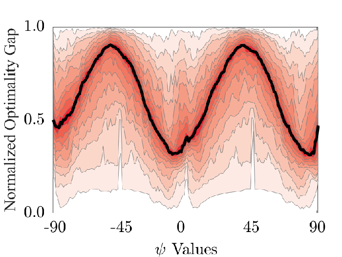
Fig. 4 shows the optimality gaps for the PGLib-OPF test cases as a function of ψ\psi, each normalized by the maximum gap for that case over all values for ψ\psi. The results in the figure were generated by sweeping ψ\psi from −90∘-90^{\circ} to 90∘90^{\circ} in steps of 0.5∘0.5^{\circ}. (The figure is exactly symmetric for values of ψ\psi from 90∘90^{\circ} to -90∘90^{\circ}.) The shaded red bands around the median line (in black) show every fifth percentile of the results.

The results in Fig. 4 indicate that good values of ψ\psi are consistent across the test systems. Thus, we suggest using ψ=80∘\psi=80^{\circ}, which is where the median of the optimality gaps over all the test cases was smallest. Moreover, the symmetry in Fig. 4 implies that selecting ψ\psi within the intervals [−90∘-90^{\circ}, −80∘-80^{\circ}], [−15∘-15^{\circ}, −5∘-5^{\circ}], and [80∘80^{\circ}, 90∘90^{\circ}] results in nearly the smallest optimality gaps for almost all of the test cases compared to the optimality gaps from the RQC relaxation using ψ∗\psi^{*}.

Refer to caption
Figure 4: Normalized optimality gap as a function of ψ\psi for PGLib-OPF cases.

Our ongoing work is generalizing the rotated QC formulation proposed in this paper by allowing for different values of ψ\psi for each line in the system in order to construct tighter envelopes (i.e., independent choices of ψl​m\psi_{lm} for each (l,m)∈ℒ(l,m)\in\mathcal{L} rather than one value of ψ\psi for the entire system). While complicating the overall formulation, this generalization simplifies the impacts from choosing each ψl​m\psi_{lm} and thus has the potential to enable analytical methods for identifying the best values for ψl​m\psi_{lm} for each (l,m)∈ℒ(l,m)\in\mathcal{L}. One possible approach is to compute the value of ψl​m\psi_{lm} that minimizes the areas of the envelopes (i.e., the yellow and red regions in Fig. 2).

VI Numerical results

This section demonstrates the effectiveness of the proposed approach using selected test cases from the PGLib-OPF v18.08 benchmark library [25]. These test cases were selected since existing relaxations fail to provide tight bounds on the best known objective values. Our implementations use Julia 0.6.4, JuMP v0.18 [26], PowerModels.jl [27], and Gurobi 8.0 as modeling tools and the solver. The results are computed using a laptop with an i7 1.80 GHz processor and 16 GB of RAM.

Table I summarizes the results from applying the QC (5), RQC (18), and TRQC (20) relaxations to selected test cases. The first column lists the test cases. The next group of columns represents optimality gaps, defined as

Optimality Gap=(Local Solution−QC BoundLocal Solution).\displaystyle\text{\emph{Optimality\penalty\ Gap}}=\left(\dfrac{\text{\emph{Local\penalty\ Solution}}-\text{\emph{QC Bound}}}{\text{\emph{Local\penalty\ Solution}}}\right). (21)

The optimality gaps are defined using the local solutions to the non-convex problem (1) from PowerModels.jl. The final group of columns shows the solver times.

Table I: Results from Applying the QC and RQC Relaxations with Various Options to Selected PGLib Test Cases
Test Cases QC Gap (%) RQC (ψ=0\psi=0) Gap (%) RQC (ψ=80∘\psi=80^{\circ}) Gap (%) RQC (ψ∗)(\psi^{*}) TRQC (ψ=80∘\psi=80^{\circ}) Gap (%) TRQC (ψ∗\psi^{*}) QC Time (sec) RQC Time (sec) TRQC Time (sec)
Gap (%) ψ∗\psi^{\ast} Gap (%) ψ∗\psi^{\ast}
case3_lmbd 00.97 00.97 00.89 00.79 −81∘-81^{\circ} 00.84 00.63 0011∘11^{\circ} 000.34 000.01 000.01
case30_ieee 18.67 14.91 13.14 12.11 0065∘65^{\circ} 13.14 11.82 −25∘-25^{\circ} 000.33 000.03 000.03
case118_ieee 00.77 00.90 00.65 00.64 0070∘70^{\circ} 00.64 00.62 0070∘70^{\circ} 000.55 000.19 000.23
case300_ieee 02.56 02.58 02.43 02.26 −13∘-13^{\circ} 02.32 02.24 −13∘-13^{\circ} 001.54 001.50 003.15
case9241_pegase 01.71 01.70 01.70 01.69 −10∘-10^{\circ} 01.70 01.69 −10∘-10^{\circ} 265.39 190.80 297.56
case3_lmbd__api 04.57 04.31 04.42 04.28 0002∘2^{\circ} 04.17 03.93 −71∘-71^{\circ} 000.51 000.01 000.01
case24_ieee_rts__api 11.02 07.83 7.51 07.24 0079∘79^{\circ} 07.31 06.98 −11∘-11^{\circ} 00.71 000.03 000.04
case39_epri__api 01.71 01.38 01.33 01.33 −11∘-11^{\circ} 01.32 01.32 0079∘79^{\circ} 000.39 000.05 000.05
case73_ieee_rts__api 09.54 08.12 07.36 07.36 −10∘-10^{\circ} 07.24 07.24 −10∘-10^{\circ} 001.00 000.29 000.37
case118_ieee__api 28.67 28.03 26.82 26.52 0−8∘-8^{\circ} 27.11 26.38 0−8∘-8^{\circ} 000.53 000.20 000.97
case179_goc__api 05.86 06.01 05.57 04.90 −81∘-81^{\circ} 04.90 04.06 −78∘-78^{\circ} 000.82 000.61 000.64
case14_ieee__sad 19.16 21.45 17.89 16.30 0077∘77^{\circ} 15.82 15.39 −12∘-12^{\circ} 000.35 000.03 000.03
case24_ieee_rts__sad 02.74 02.55 02.31 02.19 0078∘78^{\circ} 02.26 02.12 −12∘-12^{\circ} 000.40 000.05 000.06
case30_ieee__sad 05.66 05.95 04.81 04.59 −13∘-13^{\circ} 04.56 04.45 0066∘66^{\circ} 000.32 000.05 000.06
case73_ieee_rts__sad 02.37 02.24 01.98 01.90 0079∘79^{\circ} 01.84 01.82 0078∘78^{\circ} 000.41 000.28 000.41
case118_ieee__sad 06.67 08.10 05.45 05.39 0081∘81^{\circ} 05.45 05.07 0069∘69^{\circ} 000.58 000.25 000.39
case162_ieee_dtc__sad 06.22 06.30 05.65 05.59 −14∘-14^{\circ} 05.65 05.54 0076∘76^{\circ} 000.86 000.55 000.84
case300_ieee__sad 02.34 02.59 01.80 01.61 0083∘83^{\circ} 01.78 01.59 0083∘83^{\circ} 001.94 001.29 002.06

AC: AC local solution from (1), QC Gap: Optimality gap for the QC relaxation from (5), RQC Gap: Optimality gap for the Rotated QC relaxation from (18),
TRQC Gap: Optimality gap for the Tightened Rotated QC Relaxation from (20), ψ∗\psi^{*}: Use of the best ψ\psi for this case.

Comparing the second and third columns in Table I reveals that using admittances in polar form without rotation (i.e., the RQC relaxation (18) with ψ=0\psi=0) can improve the optimality gaps of some test cases (e.g., improvements of 3.76%\% and 3.19%\% for “case30_\_ieee” and “case24_\_ieee_\_rts_​_\_\_api”, respectively, relative to the original QC relaxation (5)) . However, the RQC relaxation with ψ=0\psi=0 has worse performance in other cases, such as “case300_\_ieee” and “case14_\_ieee_​_\_\_sad”, which have 0.02%\% and 2.29%\% larger optimality gaps, respectively.

Using a non-zero value for ψ\psi can improve the optimality gaps. Solving the RQC relaxation (18) with the suggested ψ=80∘\psi=80^{\circ} obtained from the empirical analysis in Section V-E results in 1.08% better optimality gaps, on average, compared to the original QC relaxation. The RQC relaxation (18) with ψ∗\psi^{*} (the best value of ψ\psi for each case) provides optimality gaps that are not worse than those obtained by the original QC relaxation (5) for all test cases, yielding an improvement of 1.36% on average compared to the original QC relaxation. As one specific example, the gap from the original QC relaxation for “case162_\_ieee_\_dtc_​_\_\_sad” is 6.22%6.22\% compared to 6.30%6.30\% for the RQC relaxation (18) with ψ=0\psi=0 relaxation (18). Use of the suggested ψ=80∘\psi=80^{\circ} reduces the gap to 5.65%\%, which is superior to the gap obtained from the QC relaxation (5). Using ψ∗\psi^{*} further reduces the optimality gap to 5.59%\%.

Enforcing the envelopes from both the original QC relaxation and the RQC relaxation, i.e., the TRQC relaxation (20), further improves the optimality gaps. Solving the TRQC relaxation (20) with the suggested ψ=80∘\psi=80^{\circ} results in 1.29% better gaps, on average, compared to the original QC relaxation. The TRQC relaxation with ψ∗\psi^{*} yields optimality gaps that are 1.571.57% and 0.210.21% better, on average, compared to the original QC relaxation and the RQC relaxation with ψ∗\psi^{*}. The additional envelopes ⟨sin⁡(θl​m)⟩S\left\langle\sin\left(\theta_{lm}\right)\right\rangle^{S} and ⟨cos⁡(θl​m)⟩C\left\langle\cos\left(\theta_{lm}\right)\right\rangle^{C} in the TRQC relaxation increase the average solver time by 2222%.

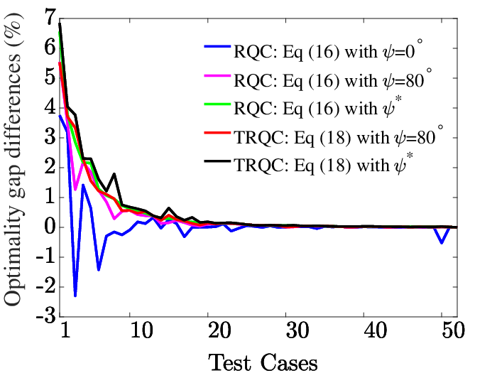
Fig. 5 visualizes the optimality gaps for variants of the QC relaxation over a range of test cases. Positive values indicate an improvement in the optimality gap of the associated variant relative to the original QC relaxation (5). The test cases are sorted in order of increasing optimality gaps obtained from the original QC relaxation. The TRQC relaxation with ψ∗\psi^{*} achieves the smallest optimality gaps. While the RQC relaxation with ψ=0\psi=0 obtains a worse optimality gap for some test cases compared to the original QC relaxation, both the RQC and TRQC relaxations with ψ∗\psi^{*} outperform the QC relaxation for all test cases. As expected from the analysis in Section V-E, applying the suggested ψ=80∘\psi=80^{\circ} results in good performance across a variety of test cases.
Refer to caption
Figure 5: Comparison of optimality gap differences with respect to the original QC relaxation (5) for different QC relaxation variants.

VII Conclusion

This paper proposes and empirically tests two improvements for strengthening QC relaxations of OPF problems by tightening the envelopes used for the trigonometric terms. The first improvement represents the line admittances in polar form. The second improvement applies a complex base power normalization with angle ψ\psi in order to rotate the arguments of the trigonometric terms. An empirical analysis is used to suggest a good value for ψ\psi. Comparison to the state-of-the-art QC relaxation reveals the effectiveness of the proposed improvements. Our ongoing work is extending the RQC relaxation to allow for distinct values of ψ\psi for each line.

Appendix A Appendices

A-A Sine and Cosine Envelopes for Extended Angle Ranges

Tables II and III on the following page extend the envelopes for the sine and cosine functions, ⟨sin⁡(x)⟩S\left\langle\sin(x)\right\rangle^{S} and ⟨cos⁡(x)⟩c\left\langle\cos(x)\right\rangle^{c}, defined in (3) and (4) in order to consider all angle ranges.

Table II: Sine Function Envelopes For Extended Angle Ranges
Envelope Interval
Sˇ≤1−1−cos⁡(xm)(xm)2​(x+3​π2)2,\widecheck{S}\leq 1-\frac{1-\cos\left({x^{m}}\right)}{\left(x^{m}\right)^{2}}\left(x+\frac{3\pi}{2}\right)^{2}, Sˇ≥sin⁡(x¯)−sin⁡(x¯)x¯−x¯​(x−x¯)+sin⁡(x¯),\widecheck{S}\geq\frac{\sin\left(\underline{x}\right)-\sin\left({\overline{x}}\right)}{{\underline{x}-\overline{x}}}\left(x-{\underline{x}}\right)+\sin\left(\underline{x}\right), xm=max⁡(|x¯+3​π2|,|x¯+3​π2|)x^{m}=\max(\left|\underline{x}+\frac{3\pi}{2}\right|,\left|\overline{x}+\frac{3\pi}{2}\right|) −2​π≤x¯-2\pi\leq\underline{x} x¯≤−π\overline{x}\leq-\pi
Sˇ≤−cos⁡(xm2)​(x+π+xm2)+sin⁡(xm2),\widecheck{S}\!\leq-\cos\left(\frac{x^{m}}{2}\right)\!\!\left(x\!+\pi+\!\frac{x^{m}}{2}\right)\!\!+\!\sin\left(\frac{x^{m}}{2}\right), Sˇ≥−cos⁡(xm2)​(x+π−xm2)−sin⁡(xm2),\widecheck{S}\!\geq-\cos\left(\frac{x^{m}}{2}\right)\!\!\left(x\!+\pi-\!\frac{x^{m}}{2}\right)\!\!-\!\sin\left(\frac{x^{m}}{2}\right), xm=max⁡(|x¯+π|,|x¯+π|)x^{m}=\max(\left|\underline{x}+\pi\right|,\left|\overline{x}+\pi\right|) −3​π2≤x¯≤−π-\frac{3\pi}{2}\leq\underline{x}\leq-\pi −π≤x¯≤−π2-\pi\leq\overline{x}\leq-\frac{\pi}{2}
Sˇ≥−(1−1−cos⁡(xm)(xm)2​(x+π2)2),\widecheck{S}\geq-\left(1-\frac{1-\cos\left({x^{m}}\right)}{\left(x^{m}\right)^{2}}\left(x+\frac{\pi}{2}\right)^{2}\right), Sˇ≤sin⁡(x¯)−sin⁡(x¯)x¯−x¯​(x−x¯)+sin⁡(x¯),\widecheck{S}\leq\frac{\sin\left(\underline{x}\right)-\sin\left({\overline{x}}\right)}{{\underline{x}-\overline{x}}}\left(x-{\underline{x}}\right)+\sin\left(\underline{x}\right), xm=max⁡(|x¯+π2|,|x¯+π2|)x^{m}=\max(\left|\underline{x}+\frac{\pi}{2}\right|,\left|\overline{x}+\frac{\pi}{2}\right|) −π≤x¯-\pi\leq\underline{x} x¯≤0\overline{x}\leq 0
Sˇ≤cos⁡(xm2)​(x−xm2)+sin⁡(xm2),\widecheck{S}\!\leq\!\cos\left(\frac{x^{m}}{2}\right)\!\!\left(x\!-\!\frac{x^{m}}{2}\right)\!\!+\!\sin\left(\frac{x^{m}}{2}\right), Sˇ≥cos⁡(xm2)​(x+xm2)−sin⁡(xm2),\widecheck{S}\!\geq\!\cos\left(\frac{x^{m}}{2}\right)\!\!\left(x\!+\!\frac{x^{m}}{2}\right)\!\!-\!\sin\left(\frac{x^{m}}{2}\right), xm=max⁡(|x¯|,|x¯|)x^{m}=\max(\left|\underline{x}\right|,\left|\overline{x}\right|) −π2≤x¯≤0-\frac{\pi}{2}\leq\underline{x}\leq 0 0≤x¯≤π20\leq\overline{x}\leq\frac{\pi}{2}
Sˇ≤1−1−cos⁡(xm)(xm)2​(x−π2)2,\widecheck{S}\leq 1-\frac{1-\cos\left({x^{m}}\right)}{\left(x^{m}\right)^{2}}\left(x-\frac{\pi}{2}\right)^{2}, Sˇ≥sin⁡(x¯)−sin⁡(x¯)x¯−x¯​(x−x¯)+sin⁡(x¯),\widecheck{S}\geq\frac{\sin\left(\underline{x}\right)-\sin\left({\overline{x}}\right)}{{\underline{x}-\overline{x}}}\left(x-{\underline{x}}\right)+\sin\left(\underline{x}\right), xm=max⁡(|x¯−π2|,|x¯−π2|)x^{m}=\max(\left|\underline{x}-\frac{\pi}{2}\right|,\left|\overline{x}-\frac{\pi}{2}\right|) 0≤x¯0\leq\underline{x} x¯≤π\overline{x}\leq\pi
Sˇ≤−cos⁡(xm2)​(x−π+xm2)+sin⁡(xm2),\widecheck{S}\!\leq-\cos\left(\frac{x^{m}}{2}\right)\!\!\left(x\!-\pi+\!\frac{x^{m}}{2}\right)\!\!+\!\sin\left(\frac{x^{m}}{2}\right), Sˇ≥−cos⁡(xm2)​(x−π−xm2)−sin⁡(xm2),\widecheck{S}\!\geq-\cos\left(\frac{x^{m}}{2}\right)\!\!\left(x\!-\pi-\!\frac{x^{m}}{2}\right)\!\!-\!\sin\left(\frac{x^{m}}{2}\right), xm=max⁡(|x¯−π|,|x¯−π|)x^{m}=\max(\left|\underline{x}-\pi\right|,\left|\overline{x}-\pi\right|) π2≤x¯≤π\frac{\pi}{2}\leq\underline{x}\leq\pi π≤x¯≤3​π2\pi\leq\overline{x}\leq\frac{3\pi}{2}
Sˇ≥−(1−1−cos⁡(xm)(xm)2​(x−3​π2)2),\widecheck{S}\geq-\left(1-\frac{1-\cos\left({x^{m}}\right)}{\left(x^{m}\right)^{2}}\left(x-\frac{3\pi}{2}\right)^{2}\right), Sˇ≤sin⁡(x¯)−sin⁡(x¯)x¯−x¯​(x−x¯)+sin⁡(x¯),\widecheck{S}\leq\frac{\sin\left(\underline{x}\right)-\sin\left({\overline{x}}\right)}{{\underline{x}-\overline{x}}}\left(x-{\underline{x}}\right)+\sin\left(\underline{x}\right), xm=max⁡(|x¯−3​π2|,|x¯−3​π2|)x^{m}=\max(\left|\underline{x}-\frac{3\pi}{2}\right|,\left|\overline{x}-\frac{3\pi}{2}\right|) π≤x¯\pi\leq\underline{x} x¯≤2​π\overline{x}\leq 2\pi
Table III: Cosine Function Envelopes For Extended Angle Ranges
Envelope Interval
Cˇ≤−cos⁡(xm2)​(x+3​π2+xm2)+sin⁡(xm2),\widecheck{C}\!\leq-\cos\left(\frac{x^{m}}{2}\right)\!\!\left(x\!+\frac{3\pi}{2}+\!\frac{x^{m}}{2}\right)\!\!+\!\sin\left(\frac{x^{m}}{2}\right), Cˇ≥−cos⁡(xm2)​(x+3​π2−xm2)−sin⁡(xm2),\widecheck{C}\!\geq-\cos\left(\frac{x^{m}}{2}\right)\!\!\left(x\!+\frac{3\pi}{2}-\!\frac{x^{m}}{2}\right)\!\!-\!\sin\left(\frac{x^{m}}{2}\right), xm=max⁡(|x¯+3​π2|,|x¯+3​π2|)x^{m}=\max(\left|\underline{x}+\frac{3\pi}{2}\right|,\left|\overline{x}+\frac{3\pi}{2}\right|) −2​π≤x¯≤−3​π2-2\pi\leq\underline{x}\leq-\frac{3\pi}{2} −3​π2​x¯≤−π-\frac{3\pi}{2}\overline{x}\leq-\pi
Cˇ≥−(1−1−cos⁡(xm)(xm)2​(x+π)2),\widecheck{C}\geq-\left(1-\frac{1-\cos\left({x^{m}}\right)}{\left(x^{m}\right)^{2}}\left(x+\pi\right)^{2}\right), Cˇ≤cos⁡(x¯)−cos⁡(x¯)x¯−x¯​(x−x¯)+cos⁡(x¯),\widecheck{C}\leq\frac{\cos\left(\underline{x}\right)-\cos\left({\overline{x}}\right)}{{\underline{x}-\overline{x}}}\left(x-{\underline{x}}\right)+\cos\left(\underline{x}\right), xm=max⁡(|x¯+π|,|x¯+π|)x^{m}=\max(\left|\underline{x}+\pi\right|,\left|\overline{x}+\pi\right|) −3​π2≤x¯-\frac{3\pi}{2}\leq\underline{x} x¯≤−π2\overline{x}\leq-\frac{\pi}{2}
Cˇ≤cos⁡(xm2)​(x+π2−xm2)+sin⁡(xm2),\widecheck{C}\!\leq\cos\left(\frac{x^{m}}{2}\right)\!\!\left(x\!+\frac{\pi}{2}-\!\frac{x^{m}}{2}\right)\!\!+\!\sin\left(\frac{x^{m}}{2}\right), Cˇ≥cos⁡(xm2)​(x+π2+xm2)−sin⁡(xm2),\widecheck{C}\!\geq\cos\left(\frac{x^{m}}{2}\right)\!\!\left(x\!+\frac{\pi}{2}+\!\frac{x^{m}}{2}\right)\!\!-\!\sin\left(\frac{x^{m}}{2}\right), xm=max⁡(|x¯+π2|,|x¯+π2|)x^{m}=\max(\left|\underline{x}+\frac{\pi}{2}\right|,\left|\overline{x}+\frac{\pi}{2}\right|) −π≤x¯≤−π2-\pi\leq\underline{x}\leq-\frac{\pi}{2} −π2≤x¯≤0-\frac{\pi}{2}\leq\overline{x}\leq 0
Cˇ≤(1−1−cos⁡(xm)(xm)2​(x+π)2),\widecheck{C}\leq\left(1-\frac{1-\cos\left({x^{m}}\right)}{\left(x^{m}\right)^{2}}\left(x+\pi\right)^{2}\right), Cˇ≥cos⁡(x¯)−cos⁡(x¯)x¯−x¯​(x−x¯)+cos⁡(x¯),\widecheck{C}\geq\frac{\cos\left(\underline{x}\right)-\cos\left({\overline{x}}\right)}{{\underline{x}-\overline{x}}}\left(x-{\underline{x}}\right)+\cos\left(\underline{x}\right), xm=max⁡(|x¯|,|x¯|)x^{m}=\max(\left|\underline{x}\right|,\left|\overline{x}\right|) −π2≤x¯-\frac{\pi}{2}\leq\underline{x} x¯≤π2\overline{x}\leq\frac{\pi}{2}
Cˇ≤−cos⁡(xm2)​(x−π2+xm2)+sin⁡(xm2),\widecheck{C}\!\leq-\cos\left(\frac{x^{m}}{2}\right)\!\!\left(x\!-\frac{\pi}{2}+\!\frac{x^{m}}{2}\right)\!\!+\!\sin\left(\frac{x^{m}}{2}\right), Cˇ≥−cos⁡(xm2)​(x−π2−xm2)−sin⁡(xm2),\widecheck{C}\!\geq-\cos\left(\frac{x^{m}}{2}\right)\!\!\left(x\!-\frac{\pi}{2}-\!\frac{x^{m}}{2}\right)\!\!-\!\sin\left(\frac{x^{m}}{2}\right), xm=max⁡(|x¯−π2|,|x¯−π2|)x^{m}=\max(\left|\underline{x}-\frac{\pi}{2}\right|,\left|\overline{x}-\frac{\pi}{2}\right|) 0≤x¯≤π20\leq\underline{x}\leq\frac{\pi}{2} π2≤x¯≤π\frac{\pi}{2}\leq\overline{x}\leq\pi
Cˇ≥−(1−1−cos⁡(xm)(xm)2​(x−π)2),\widecheck{C}\geq-\left(1-\frac{1-\cos\left({x^{m}}\right)}{\left(x^{m}\right)^{2}}\left(x-\pi\right)^{2}\right), Cˇ≤cos⁡(x¯)−cos⁡(x¯)x¯−x¯​(x−x¯)+cos⁡(x¯),\widecheck{C}\leq\frac{\cos\left(\underline{x}\right)-\cos\left({\overline{x}}\right)}{{\underline{x}-\overline{x}}}\left(x-{\underline{x}}\right)+\cos\left(\underline{x}\right), xm=max⁡(|x¯−π|,|x¯−π|)x^{m}=\max(\left|\underline{x}-\pi\right|,\left|\overline{x}-\pi\right|) π2≤x¯\frac{\pi}{2}\leq\underline{x} x¯≤3​π2\overline{x}\leq\frac{3\pi}{2}
Cˇ≤cos⁡(xm2)​(x−3​π2−xm2)+sin⁡(xm2),\widecheck{C}\!\leq\cos\left(\frac{x^{m}}{2}\right)\!\!\left(x\!-\frac{3\pi}{2}-\!\frac{x^{m}}{2}\right)\!\!+\!\sin\left(\frac{x^{m}}{2}\right), Cˇ≥cos⁡(xm2)​(x−3​π2+xm2)−sin⁡(xm2),\widecheck{C}\!\geq\cos\left(\frac{x^{m}}{2}\right)\!\!\left(x\!-\frac{3\pi}{2}+\!\frac{x^{m}}{2}\right)\!\!-\!\sin\left(\frac{x^{m}}{2}\right), xm=max⁡(|x¯−3​π2|,|x¯−3​π2|)x^{m}=\max(\left|\underline{x}-\frac{3\pi}{2}\right|,\left|\overline{x}-\frac{3\pi}{2}\right|) π≤x¯≤3​π2\pi\leq\underline{x}\leq\frac{3\pi}{2} 3​π2≤x¯≤2​π\frac{3\pi}{2}\leq\overline{x}\leq 2\pi

A-B More General Line Models

This appendix extends the paper’s results to a line model that considers transformers with a non-zero phase shift θl​ms​h​i​f​t\theta_{lm}^{shift} and/or an off-nominal voltage ratio τl​m\tau_{lm}. With this model, the complex power flows into both terminals of line (l,m)∈ℒ\left(l,m\right)\in\mathcal{L} are:

Sl​m=Vl​ej​θl​[(Yl​m​ej​δl​m+j​bc,l​m2)​Vl​ej​θlτl​m2−Yl​m​ej​δl​m​Vm​ej​θmτl​m​e−j​θl​ms​h​i​f​t]∗\displaystyle S_{lm}=V_{l}e^{j\theta_{l}}\!\left[\left(Y_{lm}e^{j\delta_{lm}}+j\frac{b_{c,lm}}{2}\right)\frac{V_{l}e^{j\theta_{l}}}{\tau_{lm}^{2}}-\frac{Y_{lm}e^{j\delta_{lm}}V_{m}e^{j\theta_{m}}}{\tau_{lm}e^{-j\theta_{lm}^{shift}}}\!\right]^{*} (22a)
Sm​l=Vm​ej​θm​[(Yl​m​ej​δl​m+j​bc,l​m2)​Vm​ej​θm−Yl​m​ej​δl​m​Vl​ej​θlτl​m​ej​θl​ms​h​i​f​t]∗\displaystyle S_{ml}=V_{m}e^{j\theta_{m}}\!\left[\left(Y_{lm}e^{j\delta_{lm}}+j\frac{b_{c,lm}}{2}\right)V_{m}e^{j\theta_{m}}\!-\!\frac{Y_{lm}e^{j\delta_{lm}}V_{l}e^{j\theta_{l}}}{\tau_{lm}e^{j\theta_{lm}^{shift}}}\!\right]^{*} (22b)

We follow the procedure in Section IV-B by applying a complex base power normalization:

S~l​m=Sl​mej​ψ=(Yl​mτl​m2​e−j⁡(δl​m+ψ)+bc,l​m2​e−j⁡(π2+ψ)τl​m2)​Vl2\displaystyle\tilde{S}_{lm}=\frac{S_{lm}}{e^{j\psi}}=\left(\frac{Y_{lm}}{\tau_{lm}^{2}}e^{-j(\delta_{lm}+\psi)}+\frac{b_{c,lm}}{2}\frac{e^{-j(\frac{\pi}{2}+\psi)}}{\tau_{lm}^{2}}\right)V_{l}^{2}
−Yl​mτl​m​Vl​Vm​ej⁡(θl​m−δl​m−θl​ms​h​i​f​t−ψ),\displaystyle\qquad\qquad\qquad\quad-\frac{Y_{lm}}{\tau_{lm}}V_{l}V_{m}e^{j(\theta_{lm}-\delta_{lm}-\theta_{lm}^{shift}-\psi)}, (23a)
S~m​l=Sm​lej​ψ=(Yl​m​e−j⁡(δl​m+ψ)+bc,l​m2​e−j⁡(π2+ψ))​Vm2\displaystyle\tilde{S}_{ml}=\frac{S_{ml}}{e^{j\psi}}=\left(Y_{lm}e^{-j(\delta_{lm}+\psi)}+\frac{b_{c,lm}}{2}e^{-j(\frac{\pi}{2}+\psi)}\right)V_{m}^{2}
−Yl​mτl​m​Vl​Vm​ej⁡(−θl​m−δl​m+θl​ms​h​i​f​t−ψ).\displaystyle\qquad\qquad\qquad\quad-\frac{Y_{lm}}{\tau_{lm}}V_{l}V_{m}e^{j(-\theta_{lm}-\delta_{lm}+\theta_{lm}^{shift}-\psi)}. (23b)

Taking the real and imaginary parts of (23) yields:

P~l​m=Re⁡(S~l​m)=(Yl​mτl​m2​cos⁡(δl​m+ψ)−bc,l​m2​τl​m2​sin⁡(ψ))​Vl2\displaystyle\!\!\!\tilde{P}_{lm}\!=\!\operatorname{Re}(\tilde{S}_{lm})\!=\!\left(\frac{Y_{lm}}{\tau_{lm}^{2}}\cos(\delta_{lm}+\psi)-\frac{b_{c,lm}}{2\tau_{lm}^{2}}\sin(\psi)\right)V_{l}^{2}
−Yl​mτl​m​Vl​Vm​cos⁡(θl​m−δl​m−θl​ms​h​i​f​t−ψ),\displaystyle\qquad\qquad-\frac{Y_{lm}}{\tau_{lm}}V_{l}V_{m}\cos(\theta_{lm}-\delta_{lm}-\theta_{lm}^{shift}-\psi), (24a)
Q~l​m=Im⁡(S~l​m)=(−Yl​mτl​m2​sin⁡(δl​m+ψ)−bc,l​m2​τl​m2​cos⁡(ψ))​Vl2\displaystyle\!\!\!\tilde{Q}_{lm}\!=\!\operatorname{Im}(\tilde{S}_{lm})\!=\!\left(-\frac{Y_{lm}}{\tau_{lm}^{2}}\sin(\delta_{lm}+\psi)\!-\!\frac{b_{c,lm}}{2\tau_{lm}^{2}}\cos(\psi)\right)\!V_{l}^{2}
−Yl​mτl​m​Vl​Vm​sin⁡(θl​m−δl​m−θl​ms​h​i​f​t−ψ),\displaystyle\qquad\quad\quad-\frac{Y_{lm}}{\tau_{lm}}V_{l}V_{m}\sin(\theta_{lm}-\delta_{lm}-\theta_{lm}^{shift}-\psi), (24b)
P~m​l=Re⁡(S~m​l)=(Yl​m​cos⁡(δl​m+ψ)−bc,l​m2​sin⁡(ψ))​Vm2\displaystyle\!\!\!\tilde{P}_{ml}\!=\!\operatorname{Re}(\tilde{S}_{ml})\!=\!\left(Y_{lm}\cos(\delta_{lm}+\psi)\!-\!\frac{b_{c,lm}}{2}\sin(\psi)\right)\!V_{m}^{2}
−Yl​mτl​m​Vm​Vl​cos⁡(θl​m+δl​m−θl​ms​h​i​f​t+ψ),\displaystyle\qquad\quad\quad-\frac{Y_{lm}}{\tau_{lm}}V_{m}V_{l}\cos(\theta_{lm}+\delta_{lm}-\theta_{lm}^{shift}+\psi), (24c)
Q~m​l=Im⁡(S~m​l)=(−Yl​m​sin⁡(δl​m+ψ)−bc,l​m2​cos⁡(ψ))​Vm2\displaystyle\!\!\!\tilde{Q}_{ml}\!=\!\operatorname{Im}(\tilde{S}_{ml})\!=\!\left(-Y_{lm}\sin(\delta_{lm}+\psi)\!-\!\frac{b_{c,lm}}{2}\cos(\psi)\right)\!V_{m}^{2}
+Yl​mτl​m​Vm​Vl​sin⁡(θl​m+δl​m−θl​ms​h​i​f​t+ψ).\displaystyle\qquad\quad\quad+\frac{Y_{lm}}{\tau_{lm}}V_{m}V_{l}\sin(\theta_{lm}+\delta_{lm}-\theta_{lm}^{shift}+\psi). (24d)

The arguments of the trigonometric terms in (24) are not independent since cos⁡(θl​m+δl​m−θl​ms​h​i​f​t+ψ)\cos(\theta_{lm}+\delta_{lm}-\theta_{lm}^{shift}+\psi) and sin⁡(θl​m+δl​m−θl​ms​h​i​f​t+ψ)\sin(\theta_{lm}+\delta_{lm}-\theta_{lm}^{shift}+\psi) are linearly related with cos⁡(θl​m−δl​m−θl​ms​h​i​f​t−ψ)\cos(\theta_{lm}-\delta_{lm}-\theta_{lm}^{shift}-\psi) and sin⁡(θl​m−δl​m−θl​ms​h​i​f​t−ψ)\sin(\theta_{lm}-\delta_{lm}-\theta_{lm}^{shift}-\psi) via the general form of (14). Extending (14) to consider off-nominal voltage ratios and non-zero phase shifts is accomplished by replacing θl​m\theta_{lm} in (14) with θl​m−θl​ms​h​i​f​t\theta_{lm}-\theta_{lm}^{shift}.

Extensions of the expressions for the squared magnitudes of the current flows in the original QC relaxation (5) and the RQC relaxation (18), ℓl​m\ell_{lm} and ℓ~l​m\tilde{\ell}_{lm}, respectively, are derived by dividing (Pl​m2+Ql​m2)(P_{lm}^{2}+Q_{lm}^{2}) and (P~l​m2+Q~l​m2)(\tilde{P}_{lm}^{2}+\tilde{Q}_{lm}^{2}) by Vl2V_{l}^{2}:

ℓl​m=(Yl​m2τl​m4−bc,l​m24​τl​m4)​Vl2+Yl​m2τl​m2​Vm2−bc,l​mτl​m2​Ql​m\displaystyle\ell_{lm}=\left(\frac{Y_{lm}^{2}}{\tau_{lm}^{4}}-\frac{b_{c,lm}^{2}}{4\tau_{lm}^{4}}\right)V_{l}^{2}+\frac{Y_{lm}^{2}}{\tau_{lm}^{2}}V_{m}^{2}-\frac{b_{c,lm}}{\tau_{lm}^{2}}Q_{lm}
−2​Yl​m2τl​m3​(cos⁡(δl​m)​cl​m+sin⁡(δl​m)​sl​m),\displaystyle\quad\quad-2\frac{Y_{lm}^{2}}{\tau_{lm}^{3}}\left(\cos(\delta_{lm})c_{lm}+\sin(\delta_{lm})s_{lm}\right), (25)
ℓ~l​m=(Yl​m2τl​m4+bc,l​m24​τl​m4−Yl​mτl​m4​bc,l​m​cos⁡(δl​m+ψ)​sin⁡(ψ)CLOSE\displaystyle\tilde{\ell}_{lm}=\bigg(\frac{Y_{lm}^{2}}{\tau_{lm}^{4}}+\frac{b_{c,lm}^{2}}{4\tau_{lm}^{4}}-\frac{Y_{lm}}{\tau_{lm}^{4}}b_{c,lm}\cos(\delta_{lm}+\psi)\sin(\psi)
OPEN+Yl​mτl​m4​bc,l​m​sin⁡(δl​m+ψ)​cos⁡(ψ))​Vl2+Yl​m2τl​m2​Vm2\displaystyle\quad\quad+\frac{Y_{lm}}{\tau_{lm}^{4}}b_{c,lm}\sin(\delta_{lm}+\psi)\cos(\psi)\bigg)V_{l}^{2}+\frac{Y_{lm}^{2}}{\tau_{lm}^{2}}V_{m}^{2}
+(Yl​mτl​m3​bc,l​m​(sin⁡(ψ)−2​Yl​m2τl​m3​cos⁡(δl​m+ψ))​c~l​mCLOSE\displaystyle\quad\quad+\left(\frac{Y_{lm}}{\tau_{lm}^{3}}b_{c,lm}(\sin(\psi)-\frac{2Y_{lm}^{2}}{\tau_{lm}^{3}}\cos(\delta_{lm}+\psi)\right)\tilde{c}_{lm}
+(Yl​mτl​m3​bc,l​m​cos⁡(ψ)+2​Yl​m2τl​m3​sin⁡(δl​m+ψ))​s~l​m\displaystyle\quad\quad+\left(\frac{Y_{lm}}{\tau_{lm}^{3}}b_{c,lm}\cos(\psi)+\frac{2Y_{lm}^{2}}{\tau_{lm}^{3}}\sin(\delta_{lm}+\psi)\right)\tilde{s}_{lm} (26)

Extending the TRQC relaxation (20) to the more general line model is achieved by modifying (19):

[cos⁡(θl​m)sin⁡(θl​m)]=Ml​m′​[sin⁡(θl​m−δl​m−ψ−θl​ms​h​i​f​t)cos⁡(θl​m−δl​m−ψ−θl​ms​h​i​f​t)],\displaystyle\begin{bmatrix}\cos(\theta_{lm})\\ \sin(\theta_{lm})\end{bmatrix}=M^{\prime}_{lm}\begin{bmatrix}\sin(\theta_{lm}-\delta_{lm}-\psi-\theta_{lm}^{shift})\\ \cos(\theta_{lm}-\delta_{lm}-\psi-\theta_{lm}^{shift})\end{bmatrix}, (27)

where the constant matrix Ml​m′M^{\prime}_{lm} is defined as

Ml​m′=\displaystyle\footnotesize M_{lm}^{\prime}= 12​([−sin⁡(δ^l​m+θl​ms​h​i​f​t)cos⁡(δ^l​m+θl​ms​h​i​f​t)cos⁡(δ^l​m+θl​ms​h​i​f​t)sin⁡(δ^l​m+θl​ms​h​i​f​t)]CLOSE\displaystyle\frac{1}{2}\left(\begin{bmatrix}-\sin(\hat{\delta}_{lm}+\theta_{lm}^{shift})&\cos(\hat{\delta}_{lm}+\theta_{lm}^{shift})\\ \cos(\hat{\delta}_{lm}+\theta_{lm}^{shift})&\sin(\hat{\delta}_{lm}+\theta_{lm}^{shift})\end{bmatrix}\right.
OPEN+[sin⁡(δ^l​m−θl​ms​h​i​f​t)cos⁡(δ^l​m−θl​ms​h​i​f​t)cos⁡(δ^l​m−θl​ms​h​i​f​t)−sin⁡(δ^l​m−θl​ms​h​i​f​t)]​[αl​mβl​m−βl​mαl​m])\displaystyle\!\!\!\!\!\!\!\!\!\!\!\!\!\!\!\!\!\!\left.+\begin{bmatrix}\sin(\hat{\delta}_{lm}-\theta_{lm}^{shift})&\cos(\hat{\delta}_{lm}-\theta_{lm}^{shift})\\ \cos(\hat{\delta}_{lm}-\theta_{lm}^{shift})&-\sin(\hat{\delta}_{lm}-\theta_{lm}^{shift})\end{bmatrix}\begin{bmatrix}\alpha_{lm}&\beta_{lm}\\ -\beta_{lm}&\alpha_{lm}\end{bmatrix}\right)

and, for notational convenience, δ^l​m=δl​m+ψ\hat{\delta}_{lm}=\delta_{lm}+\psi.

A-C Parallel Lines

In the original QC relaxation (5), the power flow equations for parallel lines between buses ll and mm shared the same envelopes, ⟨cos⁡(θl​m)⟩C\left\langle\cos(\theta_{lm})\right\rangle^{C} and ⟨sin⁡(θl​m)⟩S\left\langle\sin(\theta_{lm})\right\rangle^{S}. In the RQC relaxation (18), the arguments of the trigonometric terms for parallel lines can differ due to the inclusion of the δl​m\delta_{lm} terms. Rather than defining separate envelopes, we derive a linear relationship between the trigonometric terms for parallel lines. Let δl​m1\delta_{lm_{1}}, δl​m2\delta_{lm_{2}} and θl​m1s​h​i​f​t\theta_{lm_{1}}^{shift}, θl​m2s​h​i​f​t\theta_{lm_{2}}^{shift} be the admittance angles and phase shifts, respectively, for two parallel lines between buses ll and mm. Applying the angle sum identity yields

[sin⁡(σl​m1−θl​m)cos⁡(σl​m1−θl​m)sin⁡(σl​m2−θl​m)cos⁡(σl​m2−θl​m)]=[sin⁡(σl​m1)−cos⁡(σl​m1)cos⁡(σl​m1)sin⁡(σl​m1)sin⁡(σl​m2)−cos⁡(σl​m2)cos⁡(σl​m2)sin⁡(σl​m2)]​[cos⁡(θl​m)sin⁡(θl​m)],\small\begin{bmatrix}\sin(\sigma_{lm_{1}}-\theta_{lm})\\ \cos(\sigma_{lm_{1}}-\theta_{lm})\\ \sin(\sigma_{lm_{2}}-\theta_{lm})\\ \cos(\sigma_{lm_{2}}-\theta_{lm})\end{bmatrix}=\begin{bmatrix}\sin(\sigma_{lm_{1}})&-\cos(\sigma_{lm_{1}})\\ \cos(\sigma_{lm_{1}})&\hphantom{-}\sin(\sigma_{lm_{1}})\\ \sin(\sigma_{lm_{2}})&-\cos(\sigma_{lm_{2}})\\ \cos(\sigma_{lm_{2}})&\hphantom{-}\sin(\sigma_{lm_{2}})\end{bmatrix}\begin{bmatrix}\cos(\theta_{lm})\\ \sin(\theta_{lm})\end{bmatrix}, (28)

where, for notational convenience, σl​m1=δl​m1+θl​m1s​h​i​f​t+ψ\sigma_{lm_{1}}=\delta_{lm_{1}}+\theta_{lm_{1}}^{shift}+\psi and σl​m2=δl​m2+θl​m2s​h​i​f​t+ψ\sigma_{lm_{2}}=\delta_{lm_{2}}+\theta_{lm_{2}}^{shift}+\psi. Rearranging (28) to eliminate cos⁡(θl​m)\cos(\theta_{lm}) and sin⁡(θl​m)\sin(\theta_{lm}) yields the desired linear relationship:

[sin⁡(θl​m−σl​m2)cos⁡(θl​m−σl​m2)]=\displaystyle\begin{bmatrix}\sin(\theta_{lm}-\sigma_{lm_{2}})\\ \cos(\theta_{lm}-\sigma_{lm_{2}})\end{bmatrix}=
[cos⁡(σl​m1−σl​m2)sin⁡(σl​m1−σl​m2)−sin⁡(σl​m1−σl​m2)cos⁡(σl​m1−σl​m2)]​[sin⁡(θl​m−σl​m1)cos⁡(θl​m−σl​m1)].\displaystyle\;\begin{bmatrix}\hphantom{-}\cos(\sigma_{lm_{1}}-\sigma_{lm_{2}})&\sin(\sigma_{lm_{1}}-\sigma_{lm_{2}})\\ -\sin(\sigma_{lm_{1}}-\sigma_{lm_{2}})&\cos(\sigma_{lm_{1}}-\sigma_{lm_{2}})\end{bmatrix}\begin{bmatrix}\sin(\theta_{lm}-\sigma_{lm_{1}})\\ \cos(\theta_{lm}-\sigma_{lm_{1}})\end{bmatrix}. (29)

Since the matrix in (29) is invertible, this relationship is always well defined.

A-D Tighter Boundaries for Certain Trigonometric Envelopes

This appendix formalizes and proves a statement in Section V-A regarding the tightness of the trigonometric envelopes in the original formulation of the QC relaxation (5) and the proposed polar admittance QC formulation (18).

To assist the derivations in this appendix, we define a function F⁡(θl​m)F(\theta_{lm}) which represents the difference between the trigonometric function cos⁡(θl​m−δl​m)\cos(\theta_{lm}-\delta_{lm}) itself and the line which connects the endpoints of cos⁡(θl​m−δl​m)\cos(\theta_{lm}-\delta_{lm}) at θl​mm​i​n\theta_{lm}^{min} and θl​mm​a​x\theta_{lm}^{max}:

F⁡(θl​m)\displaystyle\noindent F(\theta_{lm}) =cos⁡(θl​m−δl​m)−cos⁡(θl​mm​a​x−δl​m)\displaystyle=\cos(\theta_{lm}-\delta_{lm})-\cos(\theta_{lm}^{max}-\delta_{lm})
−cos⁡(θl​mm​a​x−δl​m)−cos⁡(θl​mm​i​n−δl​m)θl​mm​a​x−θl​mm​i​n​(θl​m−θl​mm​a​x)\displaystyle-\frac{\cos(\theta_{lm}^{max}-\delta_{lm})-\cos(\theta_{lm}^{min}-\delta_{lm})}{\theta_{lm}^{max}-\theta_{lm}^{min}}\left(\theta_{lm}-\theta_{lm}^{max}\right) (30)

Fig. 6 shows illustrative examples of the function Yl​m​cos⁡(θl​m−δl​m)Y_{lm}\cos(\theta_{lm}-\delta_{lm}) (black curve) and the line connecting the endpoints of this function at θl​mm​i​n\theta_{lm}^{min} and θl​mm​a​x\theta_{lm}^{max} (dashed red line) on the left, with corresponding visualizations of the function F⁡(θl​m)F(\theta_{lm}) itself on the right.

cos⁡(θl​m−δl​m)\cos(\theta_{lm}-\delta_{lm}) F⁡(θl​m)F(\theta_{lm})
Refer to caption Refer to caption
(a) −165∘≤θl​m−δl​m≤15∘-165^{\circ}\leq\theta_{lm}-\delta_{lm}\leq 15^{\circ}
cos⁡(θl​m−δl​m)\cos(\theta_{lm}-\delta_{lm}) F⁡(θl​m)F(\theta_{lm})
Refer to caption Refer to caption
(b) −165∘≤θl​m−δl​m≤15∘-165^{\circ}\leq\theta_{lm}-\delta_{lm}\leq 15^{\circ}
Figure 6: The left figures show visualizations of the function cos⁡(θl​m−δl​m)\cos(\theta_{lm}-\delta_{lm}) (black curve) and the line connecting the endpoints of this function at θl​mm​i​n\theta_{lm}^{min} and θl​mm​a​x\theta_{lm}^{max} (dashed red line) for different values of δl​m\delta_{lm}, θl​mm​i​n\theta_{lm}^{min}, and θl​mm​a​x\theta_{lm}^{max}. The right figures show the corresponding function F⁡(θl​m)F(\theta_{lm}).

The derivative of F⁡(θl​m)F(\theta_{lm}) is

d​F​(θl​m)d​θl​m=−sin⁡(θl​m−δl​m)\displaystyle\frac{dF(\theta_{lm})}{d\theta_{lm}}=-\sin(\theta_{lm}-\delta_{lm})
−cos⁡(θl​mm​a​x−δl​m)−cos⁡(θl​mm​i​n−δl​m)θl​mm​a​x−θl​mm​i​n.\displaystyle\quad-\frac{\cos(\theta_{lm}^{max}-\delta_{lm})-\cos(\theta_{lm}^{min}-\delta_{lm})}{\theta_{lm}^{max}-\theta_{lm}^{min}}. (31)

A key quantity in the following proposition is the set of zeros of the derivative of F⁡(θl​m)F(\theta_{lm}), i.e., the set of solutions to d​F​(θl​m)d​θl​m=0\frac{dF(\theta_{lm})}{d\theta_{lm}}=0. This set, which we denote by 𝒵θl​mm​i​n,θl​mm​a​x,δl​m\mathcal{Z}_{\theta_{lm}^{min},\theta_{lm}^{max},\delta_{lm}} where the subscripts indicate that the set is parameterized by θl​mm​i​n\theta_{lm}^{min}, θl​mm​a​x\theta_{lm}^{max}, and δl​m\delta_{lm}, is

𝒵θl​mm​i​n,θl​mm​a​x,δl​m=\displaystyle\mathcal{Z}_{\theta_{lm}^{min},\theta_{lm}^{max},\delta_{lm}}=
{(−1)κarcsin(cos⁡(θl​mm​i​n−δl​m)−cos⁡(θl​mm​a​x−δl​m)(θl​mm​a​x−θl​mm​i​n))+πκ,\displaystyle\Big\{(-1)^{\kappa}\arcsin\left(\frac{\cos(\theta_{lm}^{min}-\delta_{lm})-\cos(\theta_{lm}^{max}-\delta_{lm})}{\left(\theta_{lm}^{max}-\theta_{lm}^{min}\right)}\right)+\pi\kappa,
κ=…,−3,−2,−1,0,1,2,3,…}.\displaystyle\qquad\kappa=\ldots,-3,-2,-1,0,1,2,3,\ldots\Big\}.

Finally, we let |⋅|\left|\,\cdot\,\right| denote the cardinality of a set.

Using these definitions, we next state and prove the following proposition.

Proposition 1.

The lower boundary of the envelope Yl​m​⟨cos⁡(θl​m−δl​m)⟩CY_{lm}\left\langle\cos(\theta_{lm}-\delta_{lm})\right\rangle^{C} is at least as tight as the lower boundary of the envelope gl​m​⟨cos⁡(θl​m)⟩C+bl​m​⟨sin⁡(θl​m)⟩Sg_{lm}\left\langle\cos(\theta_{lm})\right\rangle^{C}+b_{lm}\left\langle\sin(\theta_{lm})\right\rangle^{S} if θl​mm​i​n\theta_{lm}^{min}, θl​mm​a​x\theta_{lm}^{max}, and δl​m\delta_{lm} satisfy both of the following conditions:

|𝒵θl​mm​i​n,θl​mm​a​x,δl​m⋂{θl​mm​i​n<θl​m<θl​mm​a​x}|=1,\displaystyle\left|\mathcal{Z}_{\theta_{lm}^{min},\theta_{lm}^{max},\delta_{lm}}\bigcap\left\{\theta_{lm}^{min}<\theta_{lm}<\theta_{lm}^{max}\right\}\right|=1, (32a)
F⁡((θl​mm​a​x+θl​mm​i​n)/2)>0.\displaystyle F\left(\left(\theta_{lm}^{max}+\theta_{lm}^{min}\right)/2\right)>0. (32b)

Moreover, the upper boundary of the envelope Yl​m​⟨cos⁡(θl​m−δl​m)⟩CY_{lm}\left\langle\cos(\theta_{lm}-\delta_{lm})\right\rangle^{C} is at least as tight as the upper boundary of the envelope gl​m​⟨cos⁡(θl​m)⟩C+bl​m​⟨sin⁡(θl​m)⟩Sg_{lm}\left\langle\cos(\theta_{lm})\right\rangle^{C}+b_{lm}\left\langle\sin(\theta_{lm})\right\rangle^{S} if θl​mm​i​n\theta_{lm}^{min}, θl​mm​a​x\theta_{lm}^{max}, and δl​m\delta_{lm} satisfy both (32a) and the condition

F⁡((θl​mm​a​x+θl​mm​i​n)/2)<0.F\left(\left(\theta_{lm}^{max}+\theta_{lm}^{min}\right)/2\right)<0. (33)
Proof.

The proof is based on the following observation: if the line connecting the points (θl​mm​i​n,cos⁡(θl​mm​i​n−δl​m))(\theta_{lm}^{min},\,\cos(\theta_{lm}^{min}-\delta_{lm})) and (θl​mm​a​x,cos⁡(θl​mm​a​x−δl​m))(\theta_{lm}^{max},\,\cos(\theta_{lm}^{max}-\delta_{lm})) (i.e., the dashed red line in Fig. 6) does not intersect the function cos⁡(θl​m−δl​m)\cos(\theta_{lm}-\delta_{lm}) itself within the range θl​mm​i​n<θl​m<θl​mm​a​x\theta_{lm}^{min}<\theta_{lm}<\theta_{lm}^{max}, then this line is either the lower boundary or upper boundary of the tighest convex envelope for the function cos⁡(θl​m−δl​m)\cos(\theta_{lm}-\delta_{lm}) within this range. (For instance, the dashed red line in Fig. 6b is the lower boundary of the tighest envelope for cos⁡(θl​m−δl​m)\cos(\theta_{lm}-\delta_{lm}) within the range −165∘≤θl​m≤15∘-165^{\circ}\leq\theta_{lm}\leq 15^{\circ}.) In this case, the line is the tightest lower (upper) boundary if the function cos⁡(θl​m−δl​m)\cos(\theta_{lm}-\delta_{lm}) is above (below) the line for any point between θl​mm​i​n\theta_{lm}^{min} and θl​mm​a​x\theta_{lm}^{max} (e.g., the midpoint (θl​mm​i​n+θl​mm​a​x)/2(\theta_{lm}^{min}+\theta_{lm}^{max})/2, which is used in (32b) and (33)).

Observe that the line connecting the points (θl​mm​i​n,cos⁡(θl​mm​i​n−δl​m))(\theta_{lm}^{min},\,\cos(\theta_{lm}^{min}-\delta_{lm})) and (θl​mm​a​x,cos⁡(θl​mm​a​x−δl​m))(\theta_{lm}^{max},\,\cos(\theta_{lm}^{max}-\delta_{lm})) does not intersect the function cos⁡(θl​m−δl​m)\cos(\theta_{lm}-\delta_{lm}) between θl​mm​i​n\theta_{lm}^{min} and θl​mm​a​x\theta_{lm}^{max} if and only if F⁡(θl​m)F(\theta_{lm}) is non-zero for all θl​mm​i​n<θl​m<θl​mm​a​x\theta_{lm}^{min}<\theta_{lm}<\theta_{lm}^{max}. We next argue that this is implied by (32a).

The condition (32a) is equivalent to the existence of one critical point θl​m∗\theta_{lm}^{\ast} of the function F⁡(θl​m)F(\theta_{lm}). (i.e., the derivative of F⁡(θ)F(\theta) has a single zero, θl​m∗\theta_{lm}^{\ast}, in the range θl​mm​i​n<θl​m<θl​mm​a​x\theta_{lm}^{min}<\theta_{lm}<\theta_{lm}^{max}. Since F⁡(θl​m)F(\theta_{lm}) is continuous and F⁡(θl​mm​i​n)=F⁡(θl​mm​a​x)=0F(\theta_{lm}^{min})=F(\theta_{lm}^{max})=0, the critical point θl​m∗\theta_{lm}^{\ast} must either correspond to a minimum or maximum of F⁡(θl​m)F(\theta_{lm}). Since the function F⁡(θl​m)F(\theta_{lm}) is zero at the endpoints θl​mm​i​n\theta_{lm}^{min} and θl​mm​a​x\theta_{lm}^{max}, having a single minimum or maximum in the range θl​mm​i​n<θl​m<θl​mm​a​x\theta_{lm}^{min}<\theta_{lm}<\theta_{lm}^{max} implies that F⁡(θl​m)≠0F(\theta_{lm})\neq 0 within this range.

To complete the conditions in the proposition, (32b) and (33) determine whether the line connecting the points (θl​mm​i​n,cos⁡(θl​mm​i​n−δl​m))(\theta_{lm}^{min},\,\cos(\theta_{lm}^{min}-\delta_{lm})) and (θl​mm​a​x,cos⁡(θl​mm​a​x−δl​m))(\theta_{lm}^{max},\,\cos(\theta_{lm}^{max}-\delta_{lm})) is above or below the function cos⁡(θl​m−δl​m)\cos(\theta_{lm}-\delta_{lm}) by evaluating the function F⁡(θl​m)F(\theta_{lm}) at an arbitrary point between θl​mm​i​n\theta_{lm}^{min} and θl​mm​a​x\theta_{lm}^{max}, here selected to be the midpoint (θl​mm​i​n+θl​mm​a​x)/2\left(\theta_{lm}^{min}+\theta_{lm}^{max}\right)/2.

Since multiplication by Yl​mY_{lm} only rescales (but does not otherwise change) the envelope ⟨cos⁡(θl​m−δl​m)⟩C\left\langle\cos(\theta_{lm}-\delta_{lm})\right\rangle^{C}, the arguments above trivially extend to Yl​m​⟨cos⁡(θl​m−δl​m)⟩CY_{lm}\left\langle\cos(\theta_{lm}-\delta_{lm})\right\rangle^{C}. Moreover, since Yl​m​cos⁡(θl​m−δl​m)=gl​m​cos⁡(θl​m)+bl​m​sin⁡(θl​m)Y_{lm}\cos(\theta_{lm}-\delta_{lm})=g_{lm}\cos(\theta_{lm})+b_{lm}\sin(\theta_{lm}), the envelope gl​m​⟨cos⁡(θl​m)⟩C+bl​m​⟨sin⁡(θl​m)⟩Sg_{lm}\left\langle\cos(\theta_{lm})\right\rangle^{C}+b_{lm}\left\langle\sin(\theta_{lm})\right\rangle^{S} cannot be tighter than the tightest possible envelope for Yl​m​cos⁡(θl​m−δl​m)Y_{lm}\cos(\theta_{lm}-\delta_{lm}). Since the boundaries of Yl​m​⟨cos⁡(θl​m−δl​m)⟩CY_{lm}\left\langle\cos(\theta_{lm}-\delta_{lm})\right\rangle^{C} considered in the proof form portions of the tightest possible convex envelope for Yl​m​cos⁡(θl​m−δl​m)Y_{lm}\cos(\theta_{lm}-\delta_{lm}), they are at least as tight as the corresponding boundaries of the envelope gl​m​⟨cos⁡(θl​m)⟩C+bl​m​⟨sin⁡(θl​m)⟩Sg_{lm}\left\langle\cos(\theta_{lm})\right\rangle^{C}+b_{lm}\left\langle\sin(\theta_{lm})\right\rangle^{S}. Furthermore, the example envelopes in Fig. 2 show that the corresponding boundaries of Yl​m​⟨cos⁡(θl​m−δl​m)⟩CY_{lm}\left\langle\cos(\theta_{lm}-\delta_{lm})\right\rangle^{C} are strictly tighter than those of gl​m​⟨cos⁡(θl​m)⟩C+bl​m​⟨sin⁡(θl​m)⟩Sg_{lm}\left\langle\cos(\theta_{lm})\right\rangle^{C}+b_{lm}\left\langle\sin(\theta_{lm})\right\rangle^{S} for some values of δl​m\delta_{lm}, θl​mm​i​n\theta_{lm}^{min}, and θl​mm​a​x\theta_{lm}^{max}.

∎

We finally note that values of θl​mm​i​n\theta_{lm}^{min}, θl​mm​a​x\theta_{lm}^{max}, and δl​m\delta_{lm} such that max⁡(−90∘,−90∘+δl​m)≤θl​mm​i​n<θl​mm​a​x≤min⁡(90∘,90∘+δl​m)\max(-90^{\circ},-90^{\circ}+\delta_{lm})\leq\theta_{lm}^{min}<\theta_{lm}^{max}\leq\min(90^{\circ},90^{\circ}+\delta_{lm}) satisfy (32). Thus, the trigonometric envelopes corresponding to the polar admittance representation have lower boundaries that are at least as tight as those in the original QC relaxation for many typical values of θl​mm​i​n\theta_{lm}^{min}, θl​mm​a​x\theta_{lm}^{max}, and δl​m\delta_{lm}.

A-E Expressions for the Vertices of the Polytope Associated with the Trilinear Products

This appendix presents expressions for the vertices of the polytope consisting of the black dashed lines in Fig. 3. To compute the coordinates of these vertices (black dots in Fig. 7), we intersect the edges of the receiving end polytope, which is formed by the upper and lower bounds on the receiving end quantities, S~¯l​m(r)\vphantom{\tilde{S}_{lm}}\smash{\overline{\tilde{S}}}_{lm}^{(r)}, C~¯l​m(r)\vphantom{\tilde{C}_{lm}}\smash{\overline{\tilde{C}}}_{lm}^{(r)} and S¯~l​m(r)\vphantom{\tilde{S}_{lm}}\smash{\underline{\tilde{S}}}_{lm}^{(r)}, C¯~l​m(r)\vphantom{\tilde{C}_{lm}}\smash{\underline{\tilde{C}}}_{lm}^{(r)}, respectively, with the edges of the sending end polytope, which is formed by the upper and lower bounds on the sending end quantities S~¯l​m(s)\vphantom{\tilde{S}_{lm}}\smash{\overline{\tilde{S}}}_{lm}^{(s)}, C~¯l​m(s)\vphantom{\tilde{C}_{lm}}\smash{\overline{\tilde{C}}}_{lm}^{(s)} and S¯~l​m(s)\vphantom{\tilde{S}_{lm}}\smash{\underline{\tilde{S}}}_{lm}^{(s)}, C¯~l​m(s)\vphantom{\tilde{C}_{lm}}\smash{\underline{\tilde{C}}}_{lm}^{(s)}, respectively.

When written in terms of the sending end quantities S~l​m(s)\tilde{S}_{lm}^{(s)} and C~l​m(s)\tilde{C}_{lm}^{(s)}, the coordinates for the upper and lower bounds on the receiving end quantities are functions of ψ\psi. To write the coordinates of the vertices as functions of ψ\psi, consider the line segments labeled in Fig. 7. The yellow and purple polytopes in this figure represent the bounds on the sending and receiving end quantities, respectively. Table IV describes the relevant intersections of the line segments that form these polytopes. For the ranges of ψ\psi in the first column of Table IV, the remaining columns indicate the line segments whose intersections form the corresponding vertices. The coordinates of these intersections are given in Table V. As an example for −45∘≤ψ≤0∘-45^{\circ}\leq\psi\leq 0^{\circ}, the A′​D′A^{\prime}D^{\prime} line segment in Fig. 7 should intersect line segments AB and AD. The coordinates of these intersections are given in rows 13 and 16 of Table V.

Table IV: Line segment intersections corresponding to Fig. 7
ψ\psi (degrees) A′​B′A^{\prime}B^{\prime} B′​C′B^{\prime}C^{\prime} C′​D′C^{\prime}D^{\prime} A′​D′A^{\prime}D^{\prime}
​​​​​−45≤ψ≤0{-}45\leq\psi\leq 0 AB & BC BC & CD CD & AD AB & AD
​​​−90≤ψ≤−45\!\!{-}90\leq\psi\leq{-}45 BC & CD CD & AD AB & AD AB & BC
​​​−135≤ψ≤−90{-}135\leq\psi\leq{-}90 CD & AD AB & AD AB & BC BC & CD
​​​​​ −180≤ψ≤−135{-}180\leq\psi\leq{-}135 AB & AD AB & BC BC & CD CD & AD
​​​​​0≤ψ≤450\leq\psi\leq 45 AD & AB AB & BC BC & CD CD & AD
​​​​​45≤ψ≤9045\leq\psi\leq 90 CD & AD AD & AB AB & BC BC & CD
​​​​​90≤ψ≤13590\leq\psi\leq 135 BC & CD CD & AD AD & AB AB & BC
​​​​​135≤ψ≤180135\leq\psi\leq 180 AB & BC BC & CD CD & AD AD & AB
Table V: Coordinates of the line segment intersections in Table IV.
​​​Line Segments Coordinates of the Intersection Point
A′​B′A^{\prime}B^{\prime} & AB OPEN(αl​mβl​m​S~¯l​m(s)−βl​m​S~¯l​m(r))−OPENαl​m2​S~¯l​m(r))βl​m,S~¯l​m(s))\left(\frac{\alpha_{lm}}{\beta_{lm}}\vphantom{\tilde{S}_{lm}}\smash{\overline{\tilde{S}}}_{lm}^{(s)}-\beta_{lm}\vphantom{\tilde{S}_{lm}}\smash{\overline{\tilde{S}}}_{lm}^{(r)})-\frac{\alpha_{lm}^{2}\vphantom{\tilde{S}_{lm}}\smash{\overline{\tilde{S}}}_{lm}^{(r)})}{\beta_{lm}},\;\vphantom{\tilde{S}_{lm}}\smash{\overline{\tilde{S}}}_{lm}^{(s)}\right)
A′​B′A^{\prime}B^{\prime} & BC (C¯~l​m(s),OPENβl​m​C¯~l​m(s))αl​m+OPENβl​m2​S~¯l​m(r))αl​m+αl​m​S~¯l​m(r))\left(\vphantom{\tilde{C}_{lm}}\smash{\underline{\tilde{C}}}_{lm}^{(s)},\;\frac{\beta_{lm}\vphantom{\underline{\tilde{C}}_{lm}}\smash{\underline{\tilde{C}}}_{lm}^{(s)})}{\alpha_{lm}}+\frac{\beta_{lm}^{2}\vphantom{\tilde{S}_{lm}}\smash{\overline{\tilde{S}}}_{lm}^{(r)})}{\alpha_{lm}}+\alpha_{lm}\vphantom{\tilde{S}_{lm}}\smash{\overline{\tilde{S}}}_{lm}^{(r)}\right)
A′​B′A^{\prime}B^{\prime} & CD OPEN(αl​mβl​m​S¯~l​m(s)−βl​m​S~¯l​m(r))−OPENαl​m2​S~¯l​m(r))βl​m,S¯~l​m(s))\left(\frac{\alpha_{lm}}{\beta_{lm}}\vphantom{\tilde{S}_{lm}}\smash{\underline{\tilde{S}}}_{lm}^{(s)}-\beta_{lm}\vphantom{\tilde{S}_{lm}}\smash{\overline{\tilde{S}}}_{lm}^{(r)})-\frac{\alpha_{lm}^{2}\vphantom{\tilde{S}_{lm}}\smash{\overline{\tilde{S}}}_{lm}^{(r)})}{\beta_{lm}},\;\underline{\tilde{S}}_{lm}^{(s)}\right)
A′​B′A^{\prime}B^{\prime} & AD (C~¯l​m(s),OPENβl​m​C~¯l​m(s))αl​m+OPENβl​m2​S~¯l​m(r))αl​m+αl​m​S~¯l​m(r))\left(\vphantom{\tilde{C}_{lm}}\smash{\overline{\tilde{C}}}_{lm}^{(s)},\;\frac{\beta_{lm}\vphantom{\tilde{C}_{lm}}\smash{\overline{\tilde{C}}}_{lm}^{(s)})}{\alpha_{lm}}+\frac{\beta_{lm}^{2}\vphantom{\tilde{S}_{lm}}\smash{\overline{\tilde{S}}}_{lm}^{(r)})}{\alpha_{lm}}+\alpha_{lm}\vphantom{\tilde{S}_{lm}}\smash{\overline{\tilde{S}}}_{lm}^{(r)}\right)
B′​C′B^{\prime}C^{\prime} & BC (C¯~l​m(s),−OPENαl​m​C¯~l​m(s))βl​m+OPENαl​m2​C¯~l​m(r))βl​m+βl​m​C¯~l​m(r))\left(\vphantom{\tilde{C}_{lm}}\smash{\underline{\tilde{C}}}_{lm}^{(s)},\;-\frac{\alpha_{lm}\vphantom{\tilde{C}_{lm}}\smash{\underline{\tilde{C}}}_{lm}^{(s)})}{\beta_{lm}}+\frac{\alpha_{lm}^{2}\vphantom{\tilde{C}_{lm}}\smash{\underline{\tilde{C}}}_{lm}^{(r)})}{\beta_{lm}}+\beta_{lm}\vphantom{\tilde{C}_{lm}}\smash{\underline{\tilde{C}}}_{lm}^{(r)}\right)
B′​C′B^{\prime}C^{\prime} & CD OPEN(−βl​mαl​m​S¯~l​m(s)+αl​m​C¯~l​m(r))+OPENβl​m2​C¯~l​m(r))αl​m,S¯~l​m(s))\left(-\frac{\beta_{lm}}{\alpha_{lm}}\vphantom{\tilde{S}_{lm}}\smash{\underline{\tilde{S}}}_{lm}^{(s)}+\alpha_{lm}\vphantom{\tilde{C}_{lm}}\smash{\underline{\tilde{C}}}_{lm}^{(r)})+\frac{\beta_{lm}^{2}\vphantom{\tilde{C}_{lm}}\smash{\underline{\tilde{C}}}_{lm}^{(r)})}{\alpha_{lm}},\;\vphantom{\tilde{S}_{lm}}\smash{\underline{\tilde{S}}}_{lm}^{(s)}\right)
B′​C′B^{\prime}C^{\prime} & AB OPEN(−βl​mαl​m​S~¯l​m(s)+αl​m​C¯~l​m(r))+OPENβl​m2​C¯~l​m(r))αl​m,S~¯l​m(s))\left(-\frac{\beta_{lm}}{\alpha_{lm}}\vphantom{\tilde{S}_{lm}}\smash{\overline{\tilde{S}}}_{lm}^{(s)}+\alpha_{lm}\vphantom{\tilde{C}_{lm}}\smash{\underline{\tilde{C}}}_{lm}^{(r)})+\frac{\beta_{lm}^{2}\vphantom{\tilde{C}_{lm}}\smash{\underline{\tilde{C}}}_{lm}^{(r)})}{\alpha_{lm}},\;\vphantom{\tilde{S}_{lm}}\smash{\overline{\tilde{S}}}_{lm}^{(s)}\right)
B′​C′B^{\prime}C^{\prime} & AD (C~¯l​m(s),−OPENαl​m​C~¯l​m(s))βl​m+OPENαl​m2​C¯~l​m(r))βl​m+βl​m​C¯~l​m(r))\left(\vphantom{\tilde{C}_{lm}}\smash{\overline{\tilde{C}}}_{lm}^{(s)},\;-\frac{\alpha_{lm}\vphantom{\tilde{C}_{lm}}\smash{\overline{\tilde{C}}}_{lm}^{(s)})}{\beta_{lm}}+\frac{\alpha_{lm}^{2}\vphantom{\tilde{C}_{lm}}\smash{\underline{\tilde{C}}}_{lm}^{(r)})}{\beta_{lm}}+\beta_{lm}\vphantom{\tilde{C}_{lm}}\smash{\underline{\tilde{C}}}_{lm}^{(r)}\right)
C′​D′C^{\prime}D^{\prime} & AB OPEN(αl​mβl​m​S~¯l​m(s)−βl​m​S¯~l​m(r))−OPENαl​m2​S¯~l​m(r))βl​m,S~¯l​m(s))\left(\frac{\alpha_{lm}}{\beta_{lm}}\vphantom{\tilde{S}_{lm}}\smash{\overline{\tilde{S}}}_{lm}^{(s)}-\beta_{lm}\vphantom{\tilde{S}_{lm}}\smash{\underline{\tilde{S}}}_{lm}^{(r)})-\frac{\alpha_{lm}^{2}\vphantom{\tilde{S}_{lm}}\smash{\underline{\tilde{S}}}_{lm}^{(r)})}{\beta_{lm}},\;\vphantom{\tilde{C}_{lm}}\smash{\overline{\tilde{S}}}_{lm}^{(s)}\right)
C′​D′C^{\prime}D^{\prime} & BC (C¯~l​m(s),OPENβl​m​C¯~l​m(s))αl​m+OPENβl​m2​S¯~l​m(r))αl​m+αl​m​S¯~l​m(r))\left(\vphantom{\tilde{C}_{lm}}\smash{\underline{\tilde{C}}}_{lm}^{(s)},\;\frac{\beta_{lm}\vphantom{\tilde{C}_{lm}}\smash{\underline{\tilde{C}}}_{lm}^{(s)})}{\alpha_{lm}}+\frac{\beta_{lm}^{2}\vphantom{\tilde{S}_{lm}}\smash{\underline{\tilde{S}}}_{lm}^{(r)})}{\alpha_{lm}}+\alpha_{lm}\vphantom{\tilde{S}_{lm}}\smash{\underline{\tilde{S}}}_{lm}^{(r)}\right)
C′​D′C^{\prime}D^{\prime} & CD OPEN(αl​mβl​m​S¯~l​m(s)−βl​m​S¯~l​m(r))−OPENαl​m2​S¯~l​m(r))βl​m,S¯~l​m(s))\left(\frac{\alpha_{lm}}{\beta_{lm}}\vphantom{\tilde{C}_{lm}}\smash{\underline{\tilde{S}}}_{lm}^{(s)}-\beta_{lm}\vphantom{\tilde{S}_{lm}}\smash{\underline{\tilde{S}}}_{lm}^{(r)})-\frac{\alpha_{lm}^{2}\vphantom{\tilde{S}_{lm}}\smash{\underline{\tilde{S}}}_{lm}^{(r)})}{\beta_{lm}},\;\vphantom{\tilde{C}_{lm}}\smash{\underline{\tilde{S}}}_{lm}^{(s)}\right)
C′​D′C^{\prime}D^{\prime} & AD (C~¯l​m(s),OPENβl​m​C~¯l​m(s))αl​m+OPENβl​m2​S¯~l​m(r))αl​m+αl​m​S¯~l​m(r))\left(\vphantom{\tilde{C}_{lm}}\smash{\overline{\tilde{C}}}_{lm}^{(s)},\;\frac{\beta_{lm}\vphantom{\tilde{C}_{lm}}\smash{\overline{\tilde{C}}}_{lm}^{(s)})}{\alpha_{lm}}+\frac{\beta_{lm}^{2}\vphantom{\tilde{S}_{lm}}\smash{\underline{\tilde{S}}}_{lm}^{(r)})}{\alpha_{lm}}+\alpha_{lm}\vphantom{\tilde{S}_{lm}}\smash{\underline{\tilde{S}}}_{lm}^{(r)}\right)
A′​D′A^{\prime}D^{\prime} & AB OPEN(−βl​mαl​m​S~¯l​m(s)+αl​m​C~¯l​m(r))+OPENβl​m2​C~¯l​m(r))αl​m,S~¯l​m(s))\left(-\frac{\beta_{lm}}{\alpha_{lm}}\vphantom{\tilde{S}_{lm}}\smash{\overline{\tilde{S}}}_{lm}^{(s)}+\alpha_{lm}\vphantom{\tilde{C}_{lm}}\smash{\overline{\tilde{C}}}_{lm}^{(r)})+\frac{\beta_{lm}^{2}\vphantom{\tilde{C}_{lm}}\smash{\overline{\tilde{C}}}_{lm}^{(r)})}{\alpha_{lm}},\;\vphantom{\tilde{S}_{lm}}\smash{\overline{\tilde{S}}}_{lm}^{(s)}\right)
A′​D′A^{\prime}D^{\prime} & BC (C¯~l​m(s),−OPENαl​m​C¯~l​m(s))βl​m+OPENαl​m2​C~¯l​m(r))βl​m+βl​m​C~¯l​m(r))\left(\vphantom{\tilde{C}_{lm}}\smash{\underline{\tilde{C}}}_{lm}^{(s)},\;-\frac{\alpha_{lm}\vphantom{\tilde{C}_{lm}}\smash{\underline{\tilde{C}}}_{lm}^{(s)})}{\beta_{lm}}+\frac{\alpha_{lm}^{2}\vphantom{\tilde{C}_{lm}}\smash{\overline{\tilde{C}}}_{lm}^{(r)})}{\beta_{lm}}+\beta_{lm}\vphantom{\tilde{C}_{lm}}\smash{\overline{\tilde{C}}}_{lm}^{(r)}\right)
A′​D′A^{\prime}D^{\prime} & CD OPEN(−βl​mαl​m​S¯~l​m(s)+αl​m​C~¯l​m(r))+OPENβl​m2​C~¯l​m(r))αl​m,S¯~l​m(s))\left(-\frac{\beta_{lm}}{\alpha_{lm}}\vphantom{\tilde{S}_{lm}}\smash{\underline{\tilde{S}}}_{lm}^{(s)}+\alpha_{lm}\vphantom{\tilde{C}_{lm}}\smash{\overline{\tilde{C}}}_{lm}^{(r)})+\frac{\beta_{lm}^{2}\vphantom{\tilde{C}_{lm}}\smash{\overline{\tilde{C}}}_{lm}^{(r)})}{\alpha_{lm}},\;\vphantom{\tilde{S}_{lm}}\smash{\underline{\tilde{S}}}_{lm}^{(s)}\right)
A′​D′A^{\prime}D^{\prime} & AD (C~¯l​m(s),−OPENαl​m​C~¯l​m(s))βl​m+OPENαl​m2​C~¯l​m(r))βl​m+βl​m​C~¯l​m(r))\left(\vphantom{\tilde{C}_{lm}}\smash{\overline{\tilde{C}}}_{lm}^{(s)},\;-\frac{\alpha_{lm}\vphantom{\tilde{C}_{lm}}\smash{\overline{\tilde{C}}}_{lm}^{(s)})}{\beta_{lm}}+\frac{\alpha_{lm}^{2}\vphantom{\tilde{C}_{lm}}\smash{\overline{\tilde{C}}}_{lm}^{(r)})}{\beta_{lm}}+\beta_{lm}\vphantom{\tilde{C}_{lm}}\smash{\overline{\tilde{C}}}_{lm}^{(r)}\right)
Refer to captionA′A^{\prime}D′D^{\prime}C′C^{\prime}B′B^{\prime}ADCB
C~l​m(s)\tilde{C}_{lm}^{(s)}
S~l​m(s)\tilde{S}_{lm}^{(s)}
Figure 7: A projection of the four-dimensional polytope associated with the trilinear products between the voltage magnitudes and the trigonometric functions, expressed in terms of the sending end variables S~l​m(s)\tilde{S}_{lm}^{(s)} and C~l​m(s)\tilde{C}_{lm}^{(s)} representing cos⁡(θl​m−δl​m−ψ)\cos(\theta_{lm}-\delta_{lm}-\psi) and sin⁡(θl​m−δl​m−ψ)\sin(\theta_{lm}-\delta_{lm}-\psi). The polytope formed by intersecting the sending end polytope (ABCD) and receiving end polytope (A′​B′​C′​D′A^{\prime}B^{\prime}C^{\prime}D^{\prime}) is outlined with the dashed black lines and has vertices shown by the black dots.

References

  • [1] W. Bukhsh, A. Grothey, K. McKinnon, and P. Trodden, “Local Solutions of the Optimal Power Flow Problem,” IEEE Trans. Power Syst., vol. 28, no. 4, pp. 4780–4788, 2013.
  • [2] M. R. Narimani, D. K. Molzahn, D. Wu, and M. L. Crow, “Empirical Investigation of Non-Convexities in Optimal Power Flow Problems,” in American Control Conf. (ACC), Milwaukee, WI, USA, June 2018, pp. 3847–3854.
  • [3] D. Bienstock and A. Verma, “Strong NP-hardness of AC Power Flows Feasibility,” Oper. Res. Lett., vol. 47, no. 6, pp. 494–501, 2019.
  • [4] A. Castillo and R. O’Neill, “Survey of Approaches to Solving the ACOPF (OPF Paper 4),” FERC, Tech. Rep., Mar. 2013.
  • [5] D. K. Molzahn and I. A. Hiskens, “A Survey of Relaxations and Approximations of the Power Flow Equations,” Found. Trends Electric Energy Syst., vol. 4, no. 1-2, pp. 1–221, Feb. 2019.
  • [6] M. Lu, H. Nagarajan, R. Bent, S. D. Eksioglu, and S. J. Mason, “Tight Piecewise Convex Relaxations for Global Optimization of Optimal Power Flow,” in Power Syst. Comput. Conf. (PSCC), Dublin, Ireland, June 2018.
  • [7] J. F. Marley, D. K. Molzahn, and I. A. Hiskens, “Solving Multiperiod OPF Problems using an AC-QP Algorithm Initialized with an SOCP Relaxation,” IEEE Trans. Power Syst., vol. 32, no. 5, pp. 3538–3548, Sept. 2017.
  • [8] D. K. Molzahn and L. A. Roald, “AC Optimal Power Flow with Robust Feasibility Guarantees,” in Power Syst. Comput. Conf. (PSCC), Dublin, Ireland, June 2018.
  • [9] D. K. Molzahn, B. C. Lesieutre, and C. L. DeMarco, “A Sufficient Condition for Power Flow Insolvability With Applications to Voltage Stability Margins,” IEEE Trans. Power Syst., vol. 28, no. 3, pp. 2592–2601, Aug. 2013.
  • [10] D. K. Molzahn, “Computing the Feasible Spaces of Optimal Power Flow Problems,” IEEE Trans. Power Syst., vol. 32, no. 6, pp. 4752–4763, Nov. 2017.
  • [11] C. Coffrin, H. Hijazi, and P. Van Hentenryck, “The QC Relaxation: A Theoretical and Computational Study on Optimal Power Flow,” IEEE Trans. Power Syst., vol. 31, no. 4, pp. 3008–3018, July 2016.
  • [12] C. Coffrin, H. L. Hijazi, and P. Van Hentenryck, “Strengthening the SDP Relaxation of AC Power Flows with Convex Envelopes, Bound Tightening, and Valid Inequalities,” IEEE Trans. Power Syst., vol. 32, no. 5, pp. 3549–3558, Sept. 2017.
  • [13] C. Chen, A. Atamtürk, and S. S. Oren, “A Spatial Branch-and-Cut Algorithm for Nonconvex QCQP with Bounded Complex Variables,” Math. Prog., pp. 1–29, 2016.
  • [14] M. R. Narimani, D. K. Molzahn, and M. L. Crow, “Improving QC Relaxations of OPF Problems via Voltage Magnitude Difference Constraints and Envelopes for Trilinear Monomials,” in 20th Power Syst. Comput. Conf. (PSCC), Dublin, Ireland, June 2018.
  • [15] C. Chen, A. Atamtürk, and S. Oren, “Bound Tightening for the Alternating Current Optimal Power Flow Problem,” IEEE Trans. Power Syst., vol. 31, no. 5, pp. 3729–3736, Sept. 2016.
  • [16] B. Kocuk, S. S. Dey, and X. A. Sun, “Strong SOCP Relaxations for the Optimal Power Flow Problem,” Oper. Res., vol. 64, no. 6, pp. 1177–1196, May 2016.
  • [17] ——, “Matrix Minor Reformulation and SOCP-based Spatial Branch-and-Cut Method for the AC Optimal Power Flow Problem,” Math. Prog. Comput., vol. 10, no. 4, pp. 557–596, 2018.
  • [18] D. Shchetinin, T. T. De Rubira, and G. Hug, “Efficient Bound Tightening Techniques for Convex Relaxations of AC Optimal Power Flow,” IEEE Trans. Power Syst., vol. 34, no. 5, pp. 3848–3857, Sept. 2019.
  • [19] K. Sundar, H. Nagarajan, S. Misra, M. Lu, C. Coffrin, and R. Bent, “Optimization-Based Bound Tightening using a Strengthened QC-Relaxation of the Optimal Power Flow Problem,” arXiv:1809.04565, Sept. 2018.
  • [20] O L. Tortelli and E. M. Lourenco and A. V. Garcia and Bikash C. Pal, “Fast Decoupled Power Flow to Emerging Distribution Systems via Complex pu Normalization,” IEEE Trans. Power Syst., vol. 30, no. 3, pp. 1351–1358, 2015.
  • [21] Y. Ju, W. Wu, F. Ge, K. Ma, Y. Lin, and L. Ye, “Fast Decoupled State Estimation for Distribution Networks Considering Branch Ampere Measurements,” IEEE Trans. Smart Grid., vol. 9, no. 6, pp. 6338–6347, Nov. 2018.
  • [22] M. Farivar, C. R. Clarke, S. H. Low, and K. M. Chandy, “Inverter VAR Control for Distribution Systems with Renewables,” in IEEE Int. Conf. Smart Grid Comm. (SmartGridComm), Brussels, Belgium, Oct. 2011, pp. 457–462.
  • [23] M. R. Narimani, D. K. Molzahn, H. Nagarajan, and M. L. Crow, “Comparison of Various Trilinear Monomial Envelopes for Convex Relaxations of Optimal Power Flow Problems,” in IEEE Global Conf. Signal Infor. Proc. (GlobalSIP), Anaheim, CA, USA, Nov. 2018, pp. 865–869.
  • [24] Z. Wei, X. Chen, G. Sun, and H. Zang, “Distribution System Fast Decoupled State Estimation based on Complex PU Normalization,” in 5th Int. Conf. Electric Utility Deregulation Restructuring and Power Technologies (DRPT), Changsha, China, Nov. 2015, pp. 840–845.
  • [25] IEEE PES Task Force on Benchmarks for Validation of Emerging Power System Algorithms, “The Power Grid Library for Benchmarking AC Optimal Power Flow Algorithms,” arXiv:1908.02788, Aug. 2019. [Online]. Available: https://github.com/power-grid-lib/pglib-opf
  • [26] I. Dunning, J. Huchette, and M. Lubin, “JuMP: A Modeling Language for Mathematical Optimization,,” SIAM Rev., vol. 59, no. 2, pp. 259–320, June 2017.
  • [27] C. Coffrin, R. Bent, K. Sundar, Y. Ng, and M. Lubin, “PowerModels.jl: An Open-Source Framework for Exploring Power Flow Formulations,” in Power Syst. Comput. Conf. (PSCC), Dublin, Ireland, June 2018.