Tidal Evolution of Eccentric Binaries Driven by Convective Turbulent Viscosity2019Tidal Evolution of Eccentric Binaries Driven by Convective Turbulent Viscosity–References

Tidal dissipation shapes a variety of astrophysical binaries, causing spin synchronization of the two bodies as well as orbital decay and circularization. For example, the evolution of a stellar binary toward a common envelope episode (CEE) is affected by tides. A CEE occurs when a binary system shares a gaseous envelope. The embedded system experiences drag forces that tighten the binary orbit (Paczynski 1976; van den Heuvel 1976, e.g.). Many astronomical transients are believed to originate from systems that have experienced a CEE (Belczynski et al. 2002a; Dominik et al. 2012; Belczynski et al. 2018). Some transients may be directly associated with a CEE, e.g., recent work has suggested that luminous red novae may be caused by the ejection of a common envelope (Ivanova et al. 2013; MacLeod et al. 2017; Blagorodnova et al. 2017). A CEE can also account for the formation of compact double neutron star or black hole binaries, whose ultimate coalescence is detectable with LIGO/Virgo (Bhattacharya & van den Heuvel 1991; Belczynski et al. 2002b; Tauris & van den Heuvel 2006; Dominik et al. 2012; Vigna-Gómez et al. 2018, e.g.). In many cases, the onset and outcome of a CEE may depend on the orbital configuration of the binary when one component, a compact star, makes contact with the expanded convective envelope of the other component, a giant star. Because the pre-CEE binary can have a rather eccentric orbit, the strength of tidal dissipation in the convective envelope compared with the timescale for radius expansion of the giant star determines the orbit of the binary at the start of a CEE.

Tidal dissipation in a convective envelope can be also be important in binaries containing solar-type stars. Previous works have studied and compared different dissipation mechanisms within these stars. In the convective envelope, fundamental and inertial oscillation modes dissipate due to turbulent viscosity, while radiative diffusion operates in the stellar interior (Zahn 1977; Goodman & Oh 1997; Goodman & Dickson 1998; Savonije & Witte 2002; Ogilvie & Lin 2007, e.g.). In some cases, internal gravity waves excited at the radiative-convective boundary grow in amplitude as they travel toward the center until non-linear wave-breaking dissipates the energy and angular momentum in the wave (Goodman & Dickson 1998; Barker & Ogilvie 2010; Barker & Ogilvie 2011; Chernov et al. 2013; Ivanov et al. 2013; Bolmont & Mathis 2016; Weinberg et al. 2017; Sun et al. 2018). This effect can drive rapid orbital decay. However, when the internal gravity waves do not achieve nonlinearity, turbulent viscosity in the convective envelope is often the dominant mechanism of tidal dissipation.

A large body of work has studied the dissipation of equilibrium tides in the convective envelope of a star. An analytical treatment was first developed by Zahn 1977, using an eddy viscosity $\nu_{0}\sim v_{H}l/3$, where $l\sim H$ is the length-scale of the largest convective eddies and $v_{H}\sim(F/\rho)^{1/3}$ is the convective velocity on scale $H$ ($H$ is the pressure scale height, $F$ the convective flux, and $\rho$ the density). However, when the timescale of tidal forcing is shorter than the eddy turnover time, $\tau_{\rm eddy}=H/v_{H}$, convective eddies cannot efficiently transport energy and momentum. Zahn 1989 proposed that, in this case, the viscosity should be reduced by a linear factor of $(\omega\tau_{\rm eddy})^{-1}$, where $\omega$ is the tidal forcing frequency. In contrast, Goldreich & Nicholson 1977 suggested that the viscosity reduction should scale with $(\omega\tau_{\rm eddy})^{-2}$. Recently, numerical and analytical studies have supported a quadratic reduction factor (Penev & Sasselov 2011; Penev et al. 2011; Ogilvie & Lesur 2012; Duguid et al. 2019). A few have even discovered negative viscosities at high forcing frequencies (Ogilvie & Lesur 2012; Duguid et al. 2019).

While many previous studies have explored the effect of convective viscous dissipation on binaries in circular orbits, very few have considered the effect of frequency dependent viscosity reduction for highly eccentric binaries. A star on an eccentric orbit experiences multiple tidal forcing frequencies; the more eccentric the orbit, the wider the tidal frequency spectrum becomes. Ivanov & Papaloizou 2004 studied how different prescriptions for viscosity reduction affect the orbital evolution of a binary with a fully convective primary (e.g. a low-mass star or planet). They found that when the viscosity reduction scales more steeply than $(\omega\tau_{\rm eddy})^{-1}$, the orbital evolution of the system can change drastically.

In this paper, we study the effects of tidal dissipation due to convective turbulent viscosity in an eccentric binary. We consider both giant branch (GB) stars and solar-type stars, although our method can be applied to other types of stars with convective envelopes. In Section 2, we develop a general formalism for tidal evolution in an eccentric binary, accounting for frequency dependent damping of tidally excited oscillations. We relate this formalism to the standard weak friction treatment of the equilibrium tide (Darwin 1880; Alexander 1973; Hut 1981). In Section 3 we introduce two stellar models (a GB model and a solar-type model) and discuss the effects of frequency dependent viscosity reduction in both. In Section 4 we present results for the tidal energy and angular momentum transfer rates for both stellar models as a function of the binary orbital parameters. In Section 5 we discuss an alternative (and simpler) calculation of the transfer rates in the case of highly eccentric ($\gtrsim 0.8$) binaries before concluding in Section 6.

Consider a primary star with mass $M_{1}$ and radius $R_{1}$ in an orbit with semi-major axis $a$ and eccentricity $e$ about a secondary star, $M_{2}$. We study tidal dissipation in the convective envelope of the primary, neglecting the tide in the secondary.

In an inertial frame, the quadrupolar ($l=2$) tidal potential produced by $M_{2}$ is

where $\bm{r}=(r,\theta,\phi_{i}=\phi+\Omega_{s}t)$ is the position vector in spherical coordinates relative to the center of mass of of the primary star, and the angle $\phi$ is measured in the rotating frame of $M_{1}$, which rotates with frequency $\Omega_{s}$. Throughout this paper, we assume that the spin axis of the star is aligned with the orbital angular momentum axis (see, e.g., Lai & Wu 2006, for the gravitational potential of $M_{2}$ if the spin axis and orbital axis are misaligned.) The time-varying binary separation is $D(t)$, and $\Phi(t)$ is the orbital true anomaly. Only the $m=0,\pm 2$ terms are nonzero, with $W_{20}=\sqrt{\uppi/5}$ and $W_{2\pm 2}=\sqrt{3\uppi/10}$. The potential can be decomposed into terms with frequencies that are integer multiples of the orbital frequency, $\Omega=[G(M_{1}+M_{2})a^{-3}]^{1/2}$. In the rotating frame of the primary, we have

where

with $F_{Nm}$ defined by the expansion

and given by

where $\Psi$ is the eccentric anomaly.

The linear response of $M_{1}$ is specified by the Lagrangian displacement vector, $\mn@boldsymbol{\xi}(\bm{r},t)$, which satisfies the equation of motion

in the rotating frame of the primary, where $\bm{C}$ is a self-adjoint operator that contains the restoring forces acting on the perturbation. We can decompose the Lagrangian displacement into a sum of eigenmodes $\mn@boldsymbol{\xi}_{\alpha}(\bm{r})$ of frequency $\omega_{\alpha}$ (where $\alpha$ specifies the mode indices, which include the degree, $l$, and azimuthal index, $m$) such that (Schenk et al. 2002; Lai & Wu 2006)

where $\omega_{\alpha}$ is the mode frequency in the rotating frame. Note that the above decomposition includes both positive and negative mode frequencies. We adopt the convention that the eigenmode oscillation has the form $\mn@boldsymbol{\xi}(\bm{r},t)\propto\text{e}^{\text{i}m\phi-\text{i}\omega_{\alpha}t}$ such that positive $\omega_{\alpha}/m$ corresponds to a prograde mode. We use the normalization

where $\rho$ is the stellar density profile. With this phase space expansion, the modes satisfy the orthogonality relation $\langle\mn@boldsymbol{\xi}_{\alpha},2i\bm{\Omega_{s}}\times\mn@boldsymbol{\xi}_{\beta}\rangle+(\omega_{\alpha}+\omega_{\beta})\langle\mn@boldsymbol{\xi}_{\alpha},\mn@boldsymbol{\xi}_{\beta}\rangle=0$ for $\alpha\neq\beta$. We define

and find (Lai & Wu 2006; Fuller & Lai 2012)

where we have used

To the first order in the stellar rotation rate, $\epsilon_{\alpha}$ is the eigenfrequency of a mode in the absence of rotation, provided $\Omega_{s}\ll|\omega_{\alpha}|$. The damping rate of the forced oscillation of mode $\alpha$ at the forcing frequency $\omega_{Nm}$ is denoted by $\Gamma_{\alpha}(\omega_{Nm})$. The solution to equation (11) is

On timescales much longer than the orbital period, the energy dissipation rate in the rotating frame is given by the sum over the response to multiple forcing frequencies for oscillation modes, i.e,

In this paper, we consider tidal dissipation due to viscosity in the stellar convection zone (see Section 3). For slow rotation ($\Omega_{s}\ll|\omega_{\alpha}|$), the oscillation eigenmode is given by

where $\xi_{\alpha r}$ and $\xi_{\alpha h}$ are the radial and horizontal components of $\mn@boldsymbol{\xi}_{\alpha}({\textbf{r}})$. The viscous dissipation rate of mode $\alpha$, oscillating at the forcing frequency $\omega_{Nm}$ with amplitude $c_{\alpha N}$ is [see equation (5) of Sun et al. 2018]

where $r_{\rm conv}$ is the inner edge of the convective envelope, and $\nu$ is the isotropic kinematic viscosity. Equation (17) assumes that the flow is approximately incompressible. We define the damping rate $\gamma_{\alpha}(\omega_{Nm})$ as a relationship between $\dot{E}_{\alpha N}$ and the kinetic energy of the mode such that

with $\mn@boldsymbol{\xi}_{\alpha N}(\bm{r},t)\equiv c_{\alpha N}(t)\mn@boldsymbol{\xi}_{\alpha}(\bm{r})$. Thus,

The relationship between the two damping rates, $\Gamma_{\alpha}(\omega_{Nm})=\omega_{Nm}\gamma_{\alpha}(\omega_{Nm})/\epsilon_{\alpha}$, is discussed in the Appendix. The total energy dissipation rate in the rotating frame is then given by the sum

In the above expression, $Q_{\alpha}$ and $\bar{\epsilon}_{\alpha}=\epsilon_{\alpha}(GM_{1}/R_{1}^{3})^{-1/2}$ are dimensionless (i.e. they are in units where $G=M_{1}=R_{1}=1$). Note that if we restrict to modes with positive $\omega_{\alpha}$ in the sum, we can combine terms with $\omega_{\alpha},m,N$ and $-\omega_{-\alpha},-m,-N$. The result is to multiply equation (20) by a factor of 2. We can calculate the tidal torque on the primary, $T=\sum_{\alpha N}T_{\alpha N}$ using the relationship

Then,

where

and $\sum_{\alpha^{\prime}}$ implies that the sum is restricted to modes with $\omega_{\alpha}>0$. The tidal energy transfer rate from the orbit to the primary in the inertial frame, $\dot{E}_{\rm in}$, is related to $\dot{E}$ and $T$ via

From equations (20)-(24), we find

Together, equations (22) and (25) govern the spin and orbital evolution of the binary (see Section 2.2). ¹¹ 1 The derivation of equations (22) and (25) for the tidal torque and energy transfer rate differs from Ivanov & Papaloizou 2004 in that we use a mode decomposition (equation 8) that is rigorously valid for rotating stars.

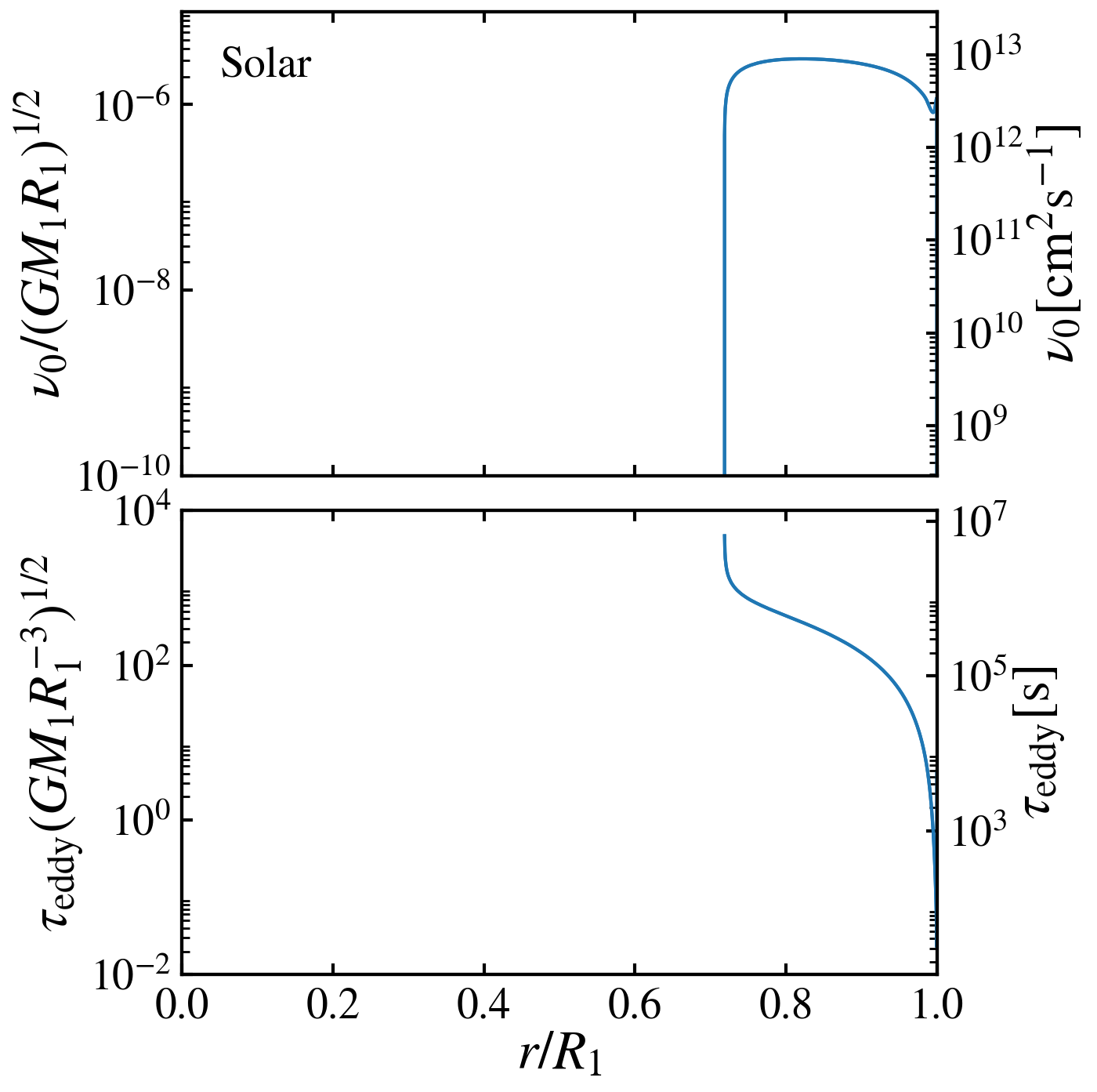
The damping rate of a forced oscillation mode depends on the convective viscosity. The standard viscosity prescription is independent of the forcing frequency and given by

where $H$ is the pressure scale height, and $v_{H}\sim(F/\rho)^{1/3}$ is the convective velocity with $F$ the convective flux. In Fig. 1, we show the viscosity and eddy turnover time $\tau_{\rm eddy}=H/v_{H}$ for two MESA-generated stellar models (Paxton et al. 2011), a $10M_{\odot}$ giant branch (GB) star and a solar-type star.

When the eddy turnover time exceeds the tidal forcing period, $\sim|\omega_{Nm}|^{-1}$, convective eddies cannot transport momentum efficiently, and the turbulent viscosity is expected to be reduced. The correct prescription for viscosity reduction has been widely discussed in the literature (see Ogilvie 2014, for a review). We adopt a quadratic reduction, first suggested by Goldreich & Nicholson 1989 and confirmed in many recent studies [see e.g. Duguid et al. 2019],

Zahn 1977, Phinney 1992 and Verbunt & Phinney 1995 provided a simple estimate of the eccentricity circularization rate for nearly circular binary stars with convective envelopes based on the “unsuppressed" viscosity $\nu_{0}$ (equation 58). To estimate the damping rate of the tidally forced f-mode (i.e. equilibrium tide), we assume $\nu_{0}\sim$ constant in the convective envelope. Then the integral in equation (19) can be approximated as

where $M_{\rm env}$ is the mass of the convective region and we have used $\nu_{0}\sim H(F/\rho)^{1/3}$ and $4\pi\rho H^{3}\sim M_{\rm env}$. Using this estimate of the equilibrium tide dissipation rate, Phinney 1992 gave the following approximation to the eccentricity damping rate (see Eq. 57)

In Fig. 2, we compare $\gamma(\omega_{Nm})$ calculated with equation (19) to $\gamma_{\rm est}$ for the MESA-generated GB and solar-type stellar models used to produce Fig. 1. We find that $\gamma(\omega_{Nm}=0)\sim\gamma_{\rm est}$. In stellar units, $\gamma_{\rm est}=0.024(GM_{1}/R_{1}^{3})^{1/2}$ for the GB model and $\gamma_{\rm est}=9.5\times 10^{-6}(GM_{1}/R_{1}^{3})^{1/2}$ for the solar-type model, corresponding to $\gamma_{\rm est}=0.20~\text{yr}^{-1}$ and $\gamma_{\rm est}=0.22~\text{yr}^{-1}$ respectively. The eddy turnover time is generally larger in the solar-type model, so it is easier for the tidal forcing period to be comparable to $\tau_{\rm eddy}$ in the depths of the convective envelope. In consequence, viscosity reduction can have a very large effect on $\gamma(\omega_{Nm})$ for the solar model, depending on $\omega_{Nm}$, and is less important for the GB model.

We have calculated $F_{T}(e,\Omega_{s}/\Omega,r_{p}/R_{1})$ and $F_{E}(e,\Omega_{s}/\Omega,r_{p}/R_{1})$ (defined in equations 43 and 44, see also equations 51-53) for the two stellar models introduced in Section 3. These dimensionless angular momentum and energy transfer rates control the synchronization rate of the primary star and the orbital evolution of the binary (see equations 54 - 56).

Typically, the timescale for the primary star to reach an equilibrium spin rate, or pseudosynchronous rate, is shorter than the timescale for orbital decay and circularization. This is clear from equations (54) - (56), where the spin evolution rate is faster than the orbital decay rate by a factor of order $\sim\mu a^{2}\Omega/I\Omega_{s}$. For an eccentric orbit, the primary star can spin-up to pseudosynchronous rotation very quickly, and it is safe to assume that the star is rotating pseudosynchronously throughout orbital decay and circularization.

When a star rotates pseudosynchrounously, it experiences no net torque. Under the weak friction approximation, the dimensionless torque is given by equation (46), so the pseudosynchronous rate is

where

is the orbit frequency at pericenter [$r_{\rm p}=(1-e)a$].

In realistic (MESA) stellar models, we use equation (51) to compute $F_{T}$ for both the standard viscosity (equation 58) and the reduced viscosity (equation 59). Figure 3 displays the results for the GB stellar model and Fig. 4 for the solar model. Equilibrium spin (pseudosynchronous rotation) corresponds to $F_{T}=0$. For the GB model, the pseudosynchronous value of $\Omega_{s}$ can be nearly a factor of two larger than the predicted $\Omega_{\rm ps}$ from weak friction theory (equation 62). Additionally, $F_{T}$ can be zero for multiple rotation rates, allowing for multiple spin equilibria (though not all of these are stable). This behavior was also noted and discussed in Storch & Lai 2014. For the GB stellar model, the two viscosity prescriptions yield similar order of magnitudes for the values of $F_{T}$. This is unsurprising as the eddy timescale $\tau_{\rm eddy}$ is generally short throughout the convective envelope of the GB star, and the viscosity is never significantly reduced (see Fig. 2).

For the solar-type stellar model, the result of $F_{T}$ with the reduced viscosity prescription is very different from either the weak friction approximation or the calculation that assumes standard (frequency-independent) viscosity (see Fig. 4). In general, $|F_{T}|$ is 1-2 orders of magnitude smaller for the reduced viscosity than for the standard viscosity. Additionally, $F_{T}$ can cross zero for slower rotation rates of nearly half of $\Omega_{\rm ps}$ (equation 62) when the viscosity is reduced.

The functions $F_{E}$ and $F_{\rm ecc}$ determine the orbital decay and circularization rates of the binary. Figure 5 displays $F_{E}$ (left column) and $F_{\rm ecc}$ (right column) as a function of pericentre distance for the GB stellar model given a rotation rate of $\Omega_{s}=0.75\Omega_{p}$, slightly below $\Omega_{\rm ps}$. Each row corresponds to a different orbital eccentricity. The functions $F_{E}(r_{p}/R_{1})$ and $F_{\rm ecc}(r_{p}/R_{1})$ have strong peaks that correspond to resonances between the mode frequencies, $\omega_{\alpha}$, and the forcing frequencies, $\omega_{Nm}$. For higher eccentricities $(e\gtrsim 0.8)$, $F_{Nm}$ can be appreciable even for $N$ of a few times larger than $\Omega_{\rm p}/\Omega=(1+e)^{1/2}/(1-e)^{3/2}$. Thus many forcing frequencies contribute significantly to $F_{E}$ and $F_{\rm ecc}$ and can dominate the sum near a resonance, as seen in the bottom row of Fig. 5. Importantly, $F_{E}$ and $F_{\rm ecc}$ can be two orders of magnitude larger than the weak friction results (equations 47 and 48) for small $r_{p}$ and high $e$. At larger pericentre distances, $F_{E}$ and $F_{\rm ecc}$ agree with the weak friction results. For the GB stellar model, the choice of viscosity prescription does not have a significant effect on the calculated orbital decay and circularization rates, as expected due to the short eddy timescale in the convective zone.

Figure 6 shows $F_{E}(r_{p}/R_{1})$ and $F_{\rm ecc}(r_{p}/R_{1})$ for the GB stellar model, as in Fig. 5, but for a larger spin rate of $\Omega_{s}=0.9\Omega_{p}$. For some combinations of $e$ and $r_{p}$, $\Omega_{s}=0.9\Omega_{p}$ exceeds the pseudosynchronous rotation rate, giving rise to orbital expansion ($F_{E}<0$, see equation 40). As an example, for $e=0.1$ (shown in the upper left panel of Fig. 6), $F_{E}$ is negative for $r_{p}/R_{1}\gtrsim 2.5-3.5$ (depending on the viscosity prescription). Otherwise, there are no qualitative differences between $F_{E}(r_{p}/R_{1})$ and $F_{\rm ecc}(r_{p}/R_{1})$ for $\Omega_{s}=0.75\Omega_{p}$ and $\Omega_{s}=0.9\Omega_{p}$.

The dimensionless orbital decay and circularization rates for the solar-type stellar model are shown in Fig. 7. For standard (frequency-independent) $\nu$, $F_{E}$ and $F_{\rm ecc}$ can be a few orders of magnitude larger than the weak friction results for small $r_{p}$ and high $e$ but agree with the weak friction results at larger $r_{p}$. Unlike for the GB model, the viscosity prescription dramatically affects the calculated $F_{E}$ and $F_{\rm ecc}$, evident in all panels of Fig. 7. Convective viscosity is inefficient in circularizing and shrinking the orbit because the eddy turnover time in the convection envelope is orders of magnitude longer than the pericentre passage time $\Omega_{p}^{-1}$. For a solar-type star, we expect orbital decay via convective dissipation to be a few orders of magnitude smaller than the weak friction prediction.

When the binary orbit is highly eccentric (with $(1-e)\ll 1$), oscillation modes in the primary star are excited at pericenter and subsequently damp as the mode oscillates freely throughout the rest of the orbit. In this regime, it is possible to calculate the tidal evolution in a different way (Lai 1997; Fuller & Lai 2012; Vick & Lai 2018, cf.).

A key quantity is the tidal energy transfer to a stellar mode (labeled $\alpha$) during the “first" pericenter passage (“first" means that there is no prior oscillation in the star). This can be computed as

with

where $r_{\rm p}=a(1-e)$, $Q_{\alpha}$ and $\epsilon_{\alpha}$ are given by equations (12) and (13), and $\sigma_{\alpha}=\omega_{\alpha}+m\Omega_{s}$ is the mode frequency in the inertial frame. Under the condition that $\sigma_{\alpha}/\Omega_{\rm p}\gtrsim$ a few, the integral $K_{2m}$ can be approximated with expressions provided in Appendix C of Lai 1997. Note that equation (64) includes contributions from both the $\omega_{\alpha},m$ and the physically identical $-\omega_{-\alpha},-m$ terms. The total energy transfer in a single pericentre passage is given by the restricted sum over positive-frequency modes, $\Delta E_{\rm in}=\sum_{\alpha^{\prime}}\Delta E_{\rm in,\alpha}$.

References

- Alexander (1973) Alexander M. E., 1973, Ap&SS, 23, 459
- Barker & Ogilvie (2010) Barker A. J., Ogilvie G. I., 2010, MNRAS, 404, 1849
- Barker & Ogilvie (2011) Barker A. J., Ogilvie G. I., 2011, MNRAS, 417, 745
- Belczynski et al. (2002a) Belczynski K., Bulik T., Rudak B., 2002a, ApJ, 571, 394
- Belczynski et al. (2002b) Belczynski K., Kalogera V., Bulik T., 2002b, ApJ, 572, 407
- Belczynski et al. (2018) Belczynski K., et al., 2018, A&A, 615, A91
- Bhattacharya & van den Heuvel (1991) Bhattacharya D., van den Heuvel E. P. J., 1991, Phys. Rep., 203, 1
- Blagorodnova et al. (2017) Blagorodnova N., et al., 2017, ApJ, 834, 107
- Bolmont & Mathis (2016) Bolmont E., Mathis S., 2016, Celestial Mechanics and Dynamical Astronomy, 126, 275
- Chernov et al. (2013) Chernov S. V., Papaloizou J. C. B., Ivanov P. B., 2013, MNRAS, 434, 1079
- Darwin (1880) Darwin G. H., 1880, Philosophical Transactions of the Royal Society of London Series I, 171, 713
- Dominik et al. (2012) Dominik M., Belczynski K., Fryer C., Holz D. E., Berti E., Bulik T., Mand el I., O’Shaughnessy R., 2012, ApJ, 759, 52
- Duguid et al. (2019) Duguid C. D., Barker A. J., Jones C. A., 2019, MNRAS, p. 2514
- Fuller & Lai (2012) Fuller J., Lai D., 2012, MNRAS, 420, 3126
- Goldreich & Nicholson (1977) Goldreich P., Nicholson P. D., 1977, Icarus, 30, 301
- Goldreich & Nicholson (1989) Goldreich P., Nicholson P. D., 1989, ApJ, 342, 1079
- Goodman & Dickson (1998) Goodman J., Dickson E. S., 1998, ApJ, 507, 938
- Goodman & Oh (1997) Goodman J., Oh S. P., 1997, ApJ, 486, 403
- Hut (1981) Hut P., 1981, A&A, 99, 126
- Ivanov & Papaloizou (2004) Ivanov P. B., Papaloizou J. C. B., 2004, MNRAS, 353, 1161
- Ivanov et al. (2013) Ivanov P. B., Papaloizou J. C. B., Chernov S. V., 2013, MNRAS, 432, 2339
- Ivanova et al. (2013) Ivanova N., et al., 2013, A&ARv, 21, 59
- Lai (1997) Lai D., 1997, ApJ, 490, 847
- Lai & Wu (2006) Lai D., Wu Y., 2006, Phys. Rev. D, 74, 024007
- MacLeod et al. (2017) MacLeod M., Macias P., Ramirez-Ruiz E., Grindlay J., Batta A., Montes G., 2017, ApJ, 835, 282
- Ogilvie (2014) Ogilvie G. I., 2014, ARA&A, 52, 171
- Ogilvie & Lesur (2012) Ogilvie G. I., Lesur G., 2012, MNRAS, 422, 1975
- Ogilvie & Lin (2007) Ogilvie G. I., Lin D. N. C., 2007, ApJ, 661, 1180
- Paczynski (1976) Paczynski B., 1976, in Eggleton P., Mitton S., Whelan J., eds, IAU Symposium Vol. 73, Structure and Evolution of Close Binary Systems. p. 75
- Paxton et al. (2011) Paxton B., Bildsten L., Dotter A., Herwig F., Lesaffre P., Timmes F., 2011, ApJS, 192, 3
- Penev & Sasselov (2011) Penev K., Sasselov D., 2011, ApJ, 731, 67
- Penev et al. (2011) Penev K., Barranco J., Sasselov D., 2011, ApJ, 734, 118
- Phinney (1992) Phinney E. S., 1992, Philosophical Transactions of the Royal Society of London Series A, 341, 39
- Price-Whelan & Goodman (2018) Price-Whelan A. M., Goodman J., 2018, ApJ, 867, 5
- Savonije & Witte (2002) Savonije G. J., Witte M. G., 2002, A&A, 386, 211
- Schenk et al. (2002) Schenk A. K., Arras P., Flanagan É. É., Teukolsky S. A., Wasserman I., 2002, Phys. Rev. D, 65, 024001
- Shporer et al. (2016) Shporer A., et al., 2016, ApJ, 829, 34
- Storch & Lai (2014) Storch N. I., Lai D., 2014, MNRAS, 438, 1526
- Sun et al. (2018) Sun M., Arras P., Weinberg N. N., Troup N. W., Majewski S. R., 2018, MNRAS, 481, 4077
- Tauris & van den Heuvel (2006) Tauris T. M., van den Heuvel E. P. J., 2006, Formation and evolution of compact stellar X-ray sources. pp 623–665
- Verbunt & Phinney (1995) Verbunt F., Phinney E. S., 1995, A&A, 296, 709
- Vick & Lai (2018) Vick M., Lai D., 2018, MNRAS, 476, 482
- Vick & Lai (2019) Vick M., Lai D., 2019, Phys. Rev. D, 100, 063001
- Vigna-Gómez et al. (2018) Vigna-Gómez A., et al., 2018, MNRAS, 481, 4009
- Weinberg et al. (2017) Weinberg N. N., Sun M., Arras P., Essick R., 2017, ApJ, 849, L11
- Witte & Savonije (1999) Witte M. G., Savonije G. J., 1999, A&A, 350, 129
- Zahn (1977) Zahn J. P., 1977, A&A, 500, 121
- Zahn (1989) Zahn J. P., 1989, A&A, 220, 112
- van den Heuvel (1976) van den Heuvel E. P. J., 1976, in Eggleton P., Mitton S., Whelan J., eds, IAU Symposium Vol. 73, Structure and Evolution of Close Binary Systems. p. 35