libmolgrid: GPU Accelerated Molecular Gridding for Deep Learning Applications

Jocelyn Sunseri David R. Koes

Abstract

There are many ways to represent a molecule as input to a machine learning model and each is associated with loss and retention of certain kinds of information. In the interest of preserving three-dimensional spatial information, including bond angles and torsions, we have developed libmolgrid, a general-purpose library for representing three-dimensional molecules using multidimensional arrays. This library also provides functionality for composing batches of data suited to machine learning workflows, including data augmentation, class balancing, and example stratification according to a regression variable or data subgroup, and it further supports temporal and spatial recurrences over that data to facilitate work with recurrent neural networks, dynamical data, and size extensive modeling. It was designed for seamless integration with popular deep learning frameworks, including Caffe, PyTorch, and Keras, providing good performance by leveraging graphical processing units (GPUs) for computationally-intensive tasks and efficient memory usage through the use of memory views over preallocated buffers. libmolgrid is a free and open source project that is actively supported, serving the growing need in the molecular modeling community for tools that streamline the process of data ingestion, representation construction, and principled machine learning model development.

keywords

Machine Learning, Deep Learning, Molecular Modeling, Python

^†^†affiliation: Department of Computational and Sytems Biology, University of Pittsburgh^†^†email: dkoes@pitt.edu

1 Introduction

The field of computational chemistry has grown in tandem with computing resourcesChemistry 1995; Mattson et al. 1995; Leach 2001; Council et al. 2003; Cramer 2004 and quantitative data about molecular structure and thermodynamicsBerman et al. 2002; Gaulton et al. 2011; Yeguas and Casado 2014; Kim et al. 2015; Goh et al. 2017; Hu and Bajorath 2017. In particular, machine learning has emerged as a novel area of study that holds great promise for unprecedented improvements in predictive capabilities for such problems as virtual screeningJorissen and Gilson 2005, binding affinity predictionBallester and Mitchell 2010; Zilian and Sotriffer 2013, pose predictionAshtawy and Mahapatra 2015; Chupakhin et al. 2013, and lead optimizationEkins et al. 2014; Yasuo et al. 2018; Zhou et al. 2019; Jiménez-Luna et al. 2019. The representation of input data can fundamentally limit or enhance the performance and applicability of machine learning algorithmsLusci et al. 2013; Duvenaud et al. 2015; Gómez-Bombarelli et al. 2018. Standard approaches to data representation include performing initial feature selection based on various types of molecular descriptors/fingerprintsXue et al. 2004; Todeschini and Consonni 2008; Unterthiner et al. 2015, including simple molecular propertiesBallester et al. 2014; Kundu et al. 2018, molecular connectivity and shapeCruciani et al. 2000; Skalic et al. 2019, electro-topological stateKatritzky and Gordeeva 1993; Durrant and McCammon 2011; Kier et al. 1999; Cang and Wei 2017, quantum chemical propertiesKarelson et al. 1996, and geometrical propertiesKatritzky and Gordeeva 1993 (or a combination of multiple of these descriptor categoriesDurrant and McCammon 2011; Wu et al. 2018); summarizing inputs using representations that are amenable to direct algorithmic analysis while preserving as much relevant information as possible, such as pairwise distances between all or selected atom groupsDeng et al. 2004; Ballester and Mitchell 2010; Gomes et al. 2017; Schütt et al. 2017, using Coulomb matrices or representations derived from themHansen et al. 2013; Hansen et al. 2015, or encoding information about local atomic environments that comprise a moleculeBehler 2011; Bartók et al. 2013; Smith et al. 2017; or using some representation of molecular structure directly as input to a machine learning algorithm such as a neural networkRagoza et al. 2017; Wallach et al. 2015; Duvenaud et al. 2015; Schütt et al. 2017; Gomes et al. 2017; Jiménez Luna et al. 2018, which extracts features and creates an internal representation of molecules itself as part of training. Commonly used input representations for the latter method include SMILES and/or InChi stringsGómez-Bombarelli et al. 2018; Winter et al. 2019, molecular graphsLusci et al. 2013; Urban et al. 2018; Duvenaud et al. 2015; Kearnes et al. 2016; Pham et al. 2018; Feinberg et al. 2018, and voxelized spatial gridsWallach et al. 2015; Ragoza et al. 2017 representing the locations of atoms.

Among this latter form of molecular representation, spatial grids possess certain virtues including minimal overt featurization by the user (theoretically permitting greater model expressiveness) and full representation of three-dimensional spatial interactions in the input. For regular cubic grids, this comes at the cost of coordinate frame dependence, which can be ameliorated by data augmentation and can also be theoretically addressed with various types of inherently equivariant network architectures or by using other types of multidimensional grids. Spatial grids have been applied successfully to tasks relevant to computational chemistry like virtual screeningWallach et al. 2015; Ragoza et al. 2017; Skalic et al. 2018, pharmacophore generationSkalic et al. 2018, molecular property predictionKajita et al. 2017; Jiménez Luna et al. 2018, molecular classificationAmidi et al. 2018; Kajita et al. 2017, protein binding site predictionHendlich et al. 1997; Jiménez et al. 2017; Jiang et al. 2019, molecular autoencodingKuzminykh et al. 2018, and generative modelingBrock et al. 2016; Brock et al. 2018; Thomas et al. 2018 by both academic and industrial groups, demonstrating their general utility.

Chemical datasets have many physical and statistical properties that prove problematic for machine learning approaches and special care must be taken to manage them. Classes are typically highly imbalanced in available datasets, with many more known inactive than active compounds for a given protein target; regression tasks may span many orders of magnitude, with nonuniform representation of the underlying chemical space at particular ranges of the regressor; and examples with matching class labels or regression target values may also be unequally sampled from other underlying classes (e.g. there may be significantly more binding affinity data available for specific proteins that have been the subject of greater medical attention, such as the estrogen receptors, or for protein classes like kinases). Chemical space is characterized by inherent symmetries that may not be reflected in a given molecular representation format. The pathologies unique to cubic grids were already mentioned, but in general all available representation methods require tradeoffs among the desired goals of maintaining symmetry to translation, rotation, and permutation while also preserving all the relevant information about chemical properties and interactions. Computational efficiency must also be prioritized if the final method is to have practical use. End users should consider the required tradeoffs and make a choice about input representation informed by their application, but once the choice is made, provided they have chosen a common representation format, the speed, accuracy, and reproducibility of their work will be enhanced if they can use a validated, open source library for input generation. By offloading data processing tasks commonly required for machine learning workflows to an open source library specialized for chemical data, computational chemists can systematically obtain better results in a transparent manner.

Using multidimensional grids (i.e. voxels) to represent atomic locations (and potentially distributions) is computationally efficient - their generation is embarrassingly parallel and therefore readily amenable to modern GPU architectures - and preserves three dimensional spatial relationships present in the original input. Their coordinate frame dependence can be removed or circumvented. But commonly available molecular parsing and conversion libraries do not yet provide gridding functionality; nor do they implement the other tasks a data scientist would require to obtain good performance on typical chemical datasets, such as the strategic resampling and data augmentation routines detailed above. Thus we abstracted the gridding and batch preparation functionality from our past work, gninaRagoza et al. 2017, into a library that can be used for general molecular modeling tasks but also interfaces naturally with popular Python deep learning libraries. Implemented in C++ with Python bindings, libmolgrid is a free and open source project intended to democratize access to molecular modeling via multidimensional arrays and to provide the additional functionality necessary to get good results from training machine learning models with typical chemical datasets.

2 Implementation

Key libmolgrid functionality is implemented in a modular fashion to ensure maximum versatility. Essential library features are abstracted into separate classes to facilitate use independently or in concert as required by a particular application.

2.1 Grids

The fundamental object used to represent data in libmolgrid is a multidimensional array which the API generically refers to as a grid. Grids are typically used during training to represent voxelized input molecules or matrices of atom coordinates and types. They can be constructed in two flavors, Grids and ManagedGrids; ManagedGrids manage their own underlying memory, while Grids function as views over a preexisting memory buffer. Figure 1 illustrates the behavior of ManagedGrids (1(a)) and Grids (1(b)). ManagedGrids can migrate data between devices, and they create a copy when converting to or from other objects that have their own memory. Grids do not own memory, instead serving as a view over the memory associated with another object that does; they do not create a copy of the buffer, rather they interact with the original buffer directly, and they cannot migrate it between devices. Grids and ManagedGrids are convertible to NumPy arrays as well as Torch tensors.

Because of automatic conversions designed for PyTorch interoperability, a user intending to leverage basic batch sampling, grid generating, and transformation capabilities provided by libmolgrid in tandem with PyTorch for neural network training can simply use Torch tensors directly, with little to no need for explicit invocation of or interaction with libmolgrid grids. Memory allocated on a GPU via a Torch tensor will remain there, with grids generated in-place. An example of this type of usage is shown in the first example in Listing 2.

A Grid may also be constructed explicitly from a Torch tensor, a NumPy array, or if necessary from a pointer to a memory buffer. Examples of constructing a Grid from a Torch tensor are shown in the second usage section in Listing 2. The third usage section shows provided functionality for copying NumPy array data to ManagedGrids, while the fourth usage section shows functionality for constructing Grid views over NumPy array data buffers. In the fourth example, note that in recent NumPy versions the default floating-point data type is float64, and therefore the user must specify float32 as the dtype if intending to copy the array data into a float rather than a double Grid.

⬇

# Usage 1: molgrid functions taking Grid objects can be passed Torch tensors directly,

# with conversions managed internally

tensor = torch.zeros(tensor_shape, dtype=torch.float32, device=’cuda’)

molgrid.gmaker.forward(batch, input_tensor)

# Usage 2: construct Grid as a view over a Torch tensor with provided helper function

tensor = torch.zeros((2,2), dtype=torch.float32, device=’cuda’)

grid = molgrid.tensor_as_grid(tensor) # dimensions and data location are inferred

# alternatively, construct Grid view over Torch tensor directly

grid = molgrid.Grid2fCUDA(tensor)

# Usage 3: copy ManagedGrid data to NumPy array

# first, construct a ManagedGrid

mgrid = molgrid.MGrid1f(batch_size)

# copy to GPU and do work on it there

mgrid.gpu()

# (do work)

# copy ManagedGrid data to a NumPy array with helper function;

# this copies data back to the CPU if necessary

array1 = mgrid.tonumpy()

# alternatively, construct NumPy array with a copy of ManagedGrid CPU data;

# must sync to CPU first

mgrid.cpu()

array2 = np.array(mgrid)

# Usage 4: construct Grid from NumPy array

array3 = np.zeros((2,2), dtype=np.float32) # must match source and destination dtypes

tensor = molgrid.Grid2f(array3)

Figure 2: Examples of Grid and ManagedGrid usage.

The explicit specialization of a grid exposed in the Python molgrid API has a naming convention that specifies its dimensionality, underlying data type, and in the case of Grids, the device where its memory buffer is located. The structure of the naming convention is [GridClass][NumDims][DataType]["CUDA" if GridClass=="Grid" and DataLoc == "GPU"]. Since ManagedGrids can migrate their data from host to device, their names do not depend on any particular data location. For example, a 1-dimensional ManagedGrid of type float is an MGrid1f, a 3-dimensional Grid of type float is a Grid3f, and a 5-dimensional Grid of type double that is a view over device data is a Grid5dCUDA.

2.2 Atom Typing

Several atom typing schemes are supported, featuring flexibility in the ways types are assigned and represented. Atoms may be typed according to XS atom typing, atomic element, or a user-provided callback function. Types may be represented by a single integer or a vector encoding. For a typical user, typing (with either index or vector types) can be performed automatically via an ExampleProvider.

2.3 Examples

Examples consist of typed coordinates that will be analyzed together, along with their labels. An Example may consist of multiple CoordinateSets (which may each utilize a different scheme for atom typing) and may be one of a sequence of Examples within a group. For example, a single Example may have a CoordinateSet for a receptor and another CoordinateSet for a ligand to be scored with that receptor, or perhaps multiple CoordinateSets corresponding to multiple poses of a particular ligand. Examples may be part of a group that will be processed in sequence, for example as input to a recurrent network; in that case distinct groups are identified with a shared integer value, and a sequence continuation flag indicates whether a given Example is a continuation of a previously observed sequence or is initiating a new one.

2.4 ExampleProvider

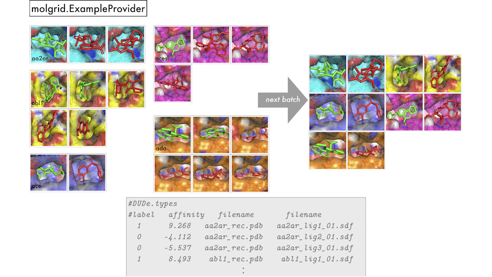
To obtain strategically sampled batches of data for training, a user can employ an ExampleProvider with custom settings. The ExampleProvider constructor is used to create an ExampleProvider with the desired settings, which can then be populated with one or more files specifying examples. The methods next and next_batch are then used to obtain the next Example or the next batch of Examples, respectively. Figure 4 shows graphically how an ExampleProvider might obtain a batch of 10 shuffled, class-balanced, receptor-stratified Examples from a larger dataset, with accompanying code.

Currently, the simplest way to initialize a provider is to populate it with one or more files that specify metadata for Examples, with one Example per line. At a high level, that line will specify class and regression target values for the Example, any group identification associated with the Example (i.e. a shared integer label identifying Examples to be processed sequentially, as with temporal data provided as input to a recurrent network), and then one or more strings identifying filenames of molecules corresponding to that Example. The default line layout is [(int)group][(float)label]*[molfile]+. An example is shown in Figure 4. In the examples we provide with our project, these files have a .types suffix.

Many ExampleProvider options govern Example resampling and the layout of the lines within the metadata file used to populate the ExampleProvider that will be used to determine how that resampling will be performed. Listing 3 shows all the available options at the time of construction. Randomization is enabled with the shuffle option; oversampling of underrepresented classes to provide equal representation from all available classes categorized by the Example label is enabled with balanced; resampling based on a specific molecule associated with an Example (determined by the first filename encountered on a given metadata line) comes from stratify_receptor (as the name suggests, this is often used to sample equally from Examples associated with different receptors); labelpos specifies the location of the binary classification label on each line of the metadata file, in terms of an index starting from 0 that numbers the entries on a line; stratify_pos similarly specifies the location of a regression target value that will be used to stratify Examples for resampling (for example a binding affinity); stratify_abs indicates that stratification of Examples based on a regression value will use the absolute value, which is useful when a negative value has a special meaning such as with a hinge loss; and stratify_min, stratify_max, and stratify_step are used to define the bins for numerical stratification of Examples.

Additional options provide customization for interpreting examples and optimizations for data I/O. When using a recurrent network for processing a sequence of data, such as the case of training with molecular dynamics frames, group_batch_size specifies the number of frames to propagate gradients through for truncated backpropagation through time and max_group_size indicates the total number of Examples associated with the largest Example group (e.g. the maximum number of frames). add_hydrogens will result in protonation of parsed molecules with OpenBabel. duplicate_first will clone the first CoordinateSet in an Example to be separately paired with each of the subsequent CoordinateSets in that Example (e.g., a single receptor structure is replicated to match different ligand poses). num_copies emits the same example multiple times (this allows the same structure to be presented to the neural network using multiple transformations in a single batch). make_vector_types will represent types as a one-hot vector rather than a single index. cache_structs will keep coordinates in memory to reduce training time. data_root allows the user to specify a shared parent directory for molecular data files, which then allows the metadata file to specify the filenames as relative paths. Finally, recmolcache and ligmolcache are binary files that store an efficient representation of all receptor and ligand files to be used for training, with each structure stored only once. These are created using the create_caches2.py script from https://github.com/gnina/scripts. Caches combine many small files into one memory mapped file resulting in a substantial I/O performance improvement and reduction in memory usage during training.

⬇

exprovider = molgrid.ExampleProvider(shuffle=False, balanced=False,

stratify_receptor=False, labelpos=0, stratify_pos=1, stratify_abs=True, stratify_min=0,

stratify_max=0, stratify_step=0, group_batch_size=1, max_group_size=0,

cache_structs=True, add_hydrogens=True, duplicate_first=False, num_copies=1,

make_vector_types=False, data_root=””, recmolcache=””, ligmolcache=””)

Figure 3: Available arguments to ExampleProvider constructor, along with their default values.

2.5 GridMaker

A GridMaker is used to generate a voxel grid from an Example, an ExampleVec, a CoordinateSet, or paired Grids of coordinates and types. GridMaker can operate directly on a user-provided Torch tensor or Grid, or it can return into a new NumPy array via GridMaker.make_ndarray or Torch tensor via GridMaker.make_tensor. GridMaker features GPU-optimized gridding that will be used if a compatible device is available. GridMaker options pertaining to the properties of the resulting grid are specified when the GridMaker is constructed, while the examples from which a grid will be generated and their instantiation properties (including any transformations) are specified by a particular invocation of GridMaker.forward. Specifically, Listing 5 shows the possible constructor arguments, including the grid resolution; dimension along each side of the cube; whether to constrain atom density values to be a binary indicator of overlapping an atom, rather than the default of a Gaussian to a multiple of the atomic radius (call this $grm$ ) and then decaying to 0 quadratically at $\frac{1+2grm^{2}}{2grm}$ ; whether to index the atomic radius array by type id (for vector types); a real-valued pre-multiplier on atomic radii, which can be used to change the size of atoms; and, if using real-valued atomic densities (rather than the alternative binary densities), the multiple of the atomic radius to which the Gaussian component of the density extends. Figure 6 shows an example of basic GridMaker usage, default-constructing a GridMaker and using it to populate a grid with densities for a batch of molecules. If desired, the values of random_translation and random_rotation can be set in the call to gmaker.forward, thereby applying random data augmentation to each example in the batch. If it is desirable to retain the applied transformation, then transformations can be created explicitly as shown in Figure 8. The GridMaker class also defines a backward function that computes atomic gradients, which can be used for tasks ranging from visualizing what a network has learned to using a trained network to optimize the coordinates and types of input molecules.

⬇

gmaker = molgrid.GridMaker(resolution=0.5, dimension=23.5, binary=False,

radius_type_indexed=False, radius_scale=1.0, gaussian_radius_multiple=1.0)

Figure 5: Available arguments to the GridMaker constructor, along with their default values.

2.6 Transformations

Data augmentation in the form of random rotations and translations of input examples can be performed by passing the desired options to GridMaker.forward as described in the previous section. Specific translations and rotations can also be applied to arbitrary Grids, CoordinateSets, or Examples by using the Transform class directly. Transforms can store specific rotations, described by a libmolgrid::Quaternion; an origin around which to rotate, described by a libmolgrid::float3, which is also interconvertible with a Python tuple; and a specific translation, expressed in terms of Cartesian coordinates and also described by a float3. Various subsets of these values may also be specified, providing for multiple transformation paradigms; usage examples are shown in Listing 7. These prove useful for sophisticated networks such as the spatial transformer. Figure 8 shows the behavior of Transform.forward, taking an input Example and returning a transformed version of that Example in transformed_example.

⬇

# Usage 1: specify a center, maximum distance for random translation,

and whether to randomly rotate

transform1 = molgrid.Transform(center=molgrid.float3(0.0,0.0,0.0), random_translate=0.0,

random_rotation=False)

qt = molgrid.Quaternion(1.0, 0.0, 0.0, 0.0)

center = molgrid.float3(0.0, 0.0, 0.0)

translate = molgrid.float3(0.0, 0.0, 0.0)

# Usage 2: specify a particular rotation, to be performed around the molecule’s center

transform2 = molgrid.Transform(qt)

# Usage 3: specify a particular rotation and the center around which it will be performed

transform3 = molgrid.Transform(qt, center)

# Usage 4: specify a particular rotation and center, along with a specific translation

transform4 = molgrid.Transform(qt, center, translate)

Figure 7: Available Transform constructors.

3 Results

We demonstrate model training with input tensors populated by molgrid and neural networks implemented using Caffe, PyTorch, and Keras with a Tensorflow backend. Figure 9 shows successful training of a basic feed-forward network on a toy dataset using each of these three deep learning frameworks to perform binary classification of active versus inactive binding modes. Timing was performed using GNU time, while memory utilization was obtained with nvidia-smi -q -i 1 -d MEMORY -l 1. The Caffe data was obtained using caffe train with the model at https://github.com/gnina/models/blob/master/affinity/affinity.model with the affinity layers removed; the PyTorch data was obtained using https://gnina.github.io/libmolgrid/tutorials/train_basic_CNN_with_PyTorch.html, run for 10,000 iterations; and the Keras data was obtained using https://gnina.github.io/libmolgrid/tutorials/train_basic_CNN_with_Tensorflow.html, run for 10,000 iterations. The metadata file for training is at https://github.com/gnina/libmolgrid/blob/master/test/data/small.types, using structures found at https://github.com/gnina/libmolgrid/tree/master/test/data/structs. molgrid is fully functional with any of these popular libraries. Its overall speed and memory footprint varies significantly with the user’s chosen library, however. As shown in Figure 10 10(a) and Figure 10 10(b), the performance when using a GPU for gridding and neural network training is much faster when using Caffe and PyTorch than it is when using Tensorflow via Keras, with modest improvements in performance for Caffe and PyTorch when using the newer Titan V GPU rather than the older GTX Titan X. This is due to libmolgrid’s ability to directly access underlying data buffers when interoperating with Caffe and PyTorch, thus avoiding unnecessary data migration between the CPU and GPU; this is not currently possible with Tensorflow, and so passes through the network involve grids being generated on the GPU by molgrid, copied into a NumPy array on the CPU, and then copied back onto the GPU by Tensorflow when training begins. This results in a significant performance penalty, with memory transfers fundamentally limiting performance; future versions of molgrid will seek to mitigate this issue with Tensorflow 2.0. The discrepancy in memory utilization shown in Figure 10 10(c) is somewhat less dramatic, but similarly, memory utilization when doing neural network training with Tensorflow is less efficient than using the other two libraries.

As an example of a more specialized task that can be performed with libmolgrid, we demonstrate training a CNN to convert voxelized atomic densities to Cartesian coordinates. Each training example consists of a single atom, provided to the network as a voxelized grid for which the network will output Cartesian coordinates. The loss function is a simple mean squared error grid loss for coordinates that fall within the grid, and a hingelike loss for coordinates outside. As shown in Figure 11 11(a), the model initially has difficulty learning because the atomic gradients only receive information from the parts of the grid that overlap an atom, but eventually converges to an accuracy significantly better than the grid resolution of 0.5Å. Example predictions are shown in Figure 11 11(b). This task could be applicable to a generative modeling workflow, and also demonstrates libmolgrid’s versatility as a molecular modeling tool.

4 Conclusion

Machine learning is a major research area within computational chemistry and drug discovery, and grid-based representation methods have been applied to many fundamental problems with great success. No standard library exists for automatically generating voxel grids or tensor representations more generally from molecular data, or for performing the basic tasks such as data augmentation that typically must be done to achieve high predictive capability on chemical datasets using these methods. This means that researchers hoping to pursue methodological advances using grid-based methods must reproduce the work of other groups and waste time with redundant programming. libmolgrid attempts to reduce the amount of irrelevant work researchers must do when pursuing advances in grid-based machine learning for molecular data, by providing an efficient, concise, and natural C++/CUDA and Python API for data resampling, grid generation, and data augmentation. It also supports spatial and temporal recurrences over input, allowing for size extensiveness even while using cubic grids (by performing a subgrid decomposition), and processing of simulation data such as molecular dynamics trajectories while preserving temporal ordering of frames, if desired. With adoption, it will also help standardize performance, enhance reproducibility, and facilitate experimentation among computational chemists interested in machine learning methods. libmolgrid support for Caffe and PyTorch is complete, while we plan to enhance Tensorflow support by taking advantage of the Tensorflow 2.0 programming model and avoiding the unnecessary data transfers that currently limit combined libmolgrid-Tensorflow performance. Other future enhancements will include the ability to generate other types of grids, for example spherical ones. Documentation, tutorials, and installation instructions are available at http://gnina.github.io/libmolgrid, while the source code along with active support can be found at https://github.com/gnina/libmolgrid.

References

Chemistry (1995) Chemistry, C. Mathematical Challenges from Theoretical/Computational Chemistry; National Academies Press, 1995.
Mattson et al. (1995) Mattson, T.; of Computers in Chemistry, A. C. S. D.; Meeting, A. C. S. N. Parallel Computing in Computational Chemistry; ACS Symposium Series v. 592; Wiley, 1995.
Leach (2001) Leach, A. Molecular Modelling: Principles and Applications; Prentice Hall, 2001.
Council et al. (2003) Council, N.; Studies, D.; Technology, B.; Century, C. Beyond the Molecular Frontier: Challenges for Chemistry and Chemical Engineering; National Academies Press, 2003.
Cramer (2004) Cramer, C. Essentials of computational chemistry: theories and models; Wiley, 2004.
Berman et al. (2002) Berman, H. M.; Battistuz, T.; Bhat, T. N.; Bluhm, W. F.; Bourne, P. E.; Burkhardt, K.; Feng, Z.; Gilliland, G. L.; Iype, L.; Jain, S., et al. The protein data bank. Acta Crystallographica Section D: Biological Crystallography 2002, 58, 899–907.
Gaulton et al. (2011) Gaulton, A.; Bellis, L. J.; Bento, A. P.; Chambers, J.; Davies, M.; Hersey, A.; Light, Y.; McGlinchey, S.; Michalovich, D.; Al-Lazikani, B., et al. ChEMBL: a large-scale bioactivity database for drug discovery. Nucleic acids research 2011, 40, D1100–D1107.
Yeguas and Casado (2014) Yeguas, V.; Casado, R. Big data issues in computational chemistry. 2014 International Conference on Future Internet of Things and Cloud. 2014; pp 389–392.
Kim et al. (2015) Kim, S.; Thiessen, P. A.; Bolton, E. E.; Chen, J.; Fu, G.; Gindulyte, A.; Han, L.; He, J.; He, S.; Shoemaker, B. A., et al. PubChem substance and compound databases. Nucleic acids research 2015, 44, D1202–D1213.
Goh et al. (2017) Goh, G. B.; Hodas, N. O.; Vishnu, A. Deep learning for computational chemistry. Journal of computational chemistry 2017, 38, 1291–1307.
Hu and Bajorath (2017) Hu, Y.; Bajorath, J. Entering the ‘big data’ era in medicinal chemistry: molecular promiscuity analysis revisited. Future science OA 2017, 3, FSO179.
Jorissen and Gilson (2005) Jorissen, R. N.; Gilson, M. K. Virtual Screening of Molecular Databases Using a Support Vector Machine. Journal of Chemical Information and Modeling 2005, 45, 549–561, [PubMed:15921445] [doi:10.1021/ci049641u].
Ballester and Mitchell (2010) Ballester, P. J.; Mitchell, J. B. O. A machine learning approach to predicting protein-ligand binding affinity with applications to molecular docking. Bioinformatics 2010, 26, 1169, [PubMed:20236947] [doi:10.1093/bioinformatics/btq112].
Zilian and Sotriffer (2013) Zilian, D.; Sotriffer, C. A. SFCscore RF: a random forest-based scoring function for improved affinity prediction of protein–ligand complexes. Journal of chemical information and modeling 2013, 53, 1923–1933, [PubMed:23705795] [doi:10.1021/ci400120b].
Ashtawy and Mahapatra (2015) Ashtawy, H. M.; Mahapatra, N. R. Machine-learning scoring functions for identifying native poses of ligands docked to known and novel proteins. BMC Bioinformatics 2015, 16, 1–17, [PubMed:25916860] [PubMed Central:PMC4416170] [doi:10.1186/1471-2105-16-S6-S3].
Chupakhin et al. (2013) Chupakhin, V.; Marcou, G.; Baskin, I.; Varnek, A.; Rognan, D. Predicting ligand binding modes from neural networks trained on protein–ligand interaction fingerprints. Journal of chemical information and modeling 2013, 53, 763–772, [PubMed:23480697] [doi:10.1021/ci300200r].
Ekins et al. (2014) Ekins, S.; Freundlich, J. S.; Hobrath, J. V.; White, E. L.; Reynolds, R. C. Combining computational methods for hit to lead optimization in Mycobacterium tuberculosis drug discovery. Pharmaceutical research 2014, 31, 414–435.
Yasuo et al. (2018) Yasuo, N.; Watanabe, K.; Hara, H.; Rikimaru, K.; Sekijima, M. Predicting Strategies for Lead Optimization via Learning to Rank. IPSJ Transactions on Bioinformatics 2018, 11, 41–47.
Zhou et al. (2019) Zhou, Z.; Kearnes, S.; Li, L.; Zare, R. N.; Riley, P. Optimization of molecules via deep reinforcement learning. Scientific reports 2019, 9, 1–10.
Jiménez-Luna et al. (2019) Jiménez-Luna, J.; Pérez-Benito, L.; Martínez-Rosell, G.; Sciabola, S.; Torella, R.; Tresadern, G.; De Fabritiis, G. DeltaDelta neural networks for lead optimization of small molecule potency. Chemical Science 2019,
Lusci et al. (2013) Lusci, A.; Pollastri, G.; Baldi, P. Deep architectures and deep learning in chemoinformatics: the prediction of aqueous solubility for drug-like molecules. Journal of chemical information and modeling 2013, 53, 1563–1575.
Duvenaud et al. (2015) Duvenaud, D. K.; Maclaurin, D.; Iparraguirre, J.; Bombarell, R.; Hirzel, T.; Aspuru-Guzik, A.; Adams, R. P. Convolutional networks on graphs for learning molecular fingerprints. Advances in neural information processing systems. 2015; pp 2224–2232.
Gómez-Bombarelli et al. (2018) Gómez-Bombarelli, R.; Wei, J. N.; Duvenaud, D.; Hernández-Lobato, J. M.; Sánchez-Lengeling, B.; Sheberla, D.; Aguilera-Iparraguirre, J.; Hirzel, T. D.; Adams, R. P.; Aspuru-Guzik, A. Automatic chemical design using a data-driven continuous representation of molecules. ACS central science 2018, 4, 268–276.
Xue et al. (2004) Xue, Y.; Yap, C. W.; Sun, L. Z.; Cao, Z. W.; Wang, J.; Chen, Y. Z. Prediction of P-glycoprotein substrates by a support vector machine approach. Journal of chemical information and computer sciences 2004, 44, 1497–1505.
Todeschini and Consonni (2008) Todeschini, R.; Consonni, V. Handbook of molecular descriptors; John Wiley & Sons, 2008; Vol. 11.
Unterthiner et al. (2015) Unterthiner, T.; Mayr, A.; Klambauer, G.; Hochreiter, S. Toxicity prediction using deep learning. arXiv preprint arXiv:1503.01445 2015,
Ballester et al. (2014) Ballester, P. J.; Schreyer, A.; Blundell, T. L. Does a more precise chemical description of protein–ligand complexes lead to more accurate prediction of binding affinity? Journal of chemical information and modeling 2014, 54, 944–955.
Kundu et al. (2018) Kundu, I.; Paul, G.; Banerjee, R. A machine learning approach towards the prediction of protein–ligand binding affinity based on fundamental molecular properties. RSC advances 2018, 8, 12127–12137.
Cruciani et al. (2000) Cruciani, G.; Pastor, M.; Guba, W. VolSurf: a new tool for the pharmacokinetic optimization of lead compounds. European Journal of Pharmaceutical Sciences 2000, 11, S29–S39.
Skalic et al. (2019) Skalic, M.; Jiménez, J.; Sabbadin, D.; De Fabritiis, G. Shape-Based Generative Modeling for de Novo Drug Design. Journal of chemical information and modeling 2019, 59, 1205–1214.
Katritzky and Gordeeva (1993) Katritzky, A. R.; Gordeeva, E. V. Traditional topological indexes vs electronic, geometrical, and combined molecular descriptors in QSAR/QSPR research. Journal of chemical information and computer sciences 1993, 33, 835–857.
Durrant and McCammon (2011) Durrant, J. D.; McCammon, J. A. BINANA: a novel algorithm for ligand-binding characterization. Journal of Molecular Graphics and Modelling 2011, 29, 888–893.
Kier et al. (1999) Kier, L. B.; Hall, L. H., et al. Molecular structure description; Academic, 1999.
Cang and Wei (2017) Cang, Z.; Wei, G.-W. TopologyNet: Topology based deep convolutional and multi-task neural networks for biomolecular property predictions. PLoS computational biology 2017, 13, e1005690.
Karelson et al. (1996) Karelson, M.; Lobanov, V. S.; Katritzky, A. R. Quantum-chemical descriptors in QSAR/QSPR studies. Chemical reviews 1996, 96, 1027–1044.
Durrant and McCammon (2011) Durrant, J. D.; McCammon, J. A. NNScore 2.0: a neural-network receptor–ligand scoring function. Journal of chemical information and modeling 2011, 51, 2897–2903.
Wu et al. (2018) Wu, Z.; Ramsundar, B.; Feinberg, E. N.; Gomes, J.; Geniesse, C.; Pappu, A. S.; Leswing, K.; Pande, V. MoleculeNet: a benchmark for molecular machine learning. Chemical science 2018, 9, 513–530.
Deng et al. (2004) Deng, W.; Breneman, C.; Embrechts, M. J. Predicting protein- ligand binding affinities using novel geometrical descriptors and machine-learning methods. Journal of chemical information and computer sciences 2004, 44, 699–703.
Gomes et al. (2017) Gomes, J.; Ramsundar, B.; Feinberg, E. N.; Pande, V. S. Atomic convolutional networks for predicting protein-ligand binding affinity. arXiv preprint arXiv:1703.10603 2017,
Schütt et al. (2017) Schütt, K.; Kindermans, P.-J.; Felix, H. E. S.; Chmiela, S.; Tkatchenko, A.; Müller, K.-R. Schnet: A continuous-filter convolutional neural network for modeling quantum interactions. Advances in Neural Information Processing Systems. 2017; pp 991–1001.
Hansen et al. (2013) Hansen, K.; Montavon, G.; Biegler, F.; Fazli, S.; Rupp, M.; Scheffler, M.; Von Lilienfeld, O. A.; Tkatchenko, A.; Müller, K.-R. Assessment and validation of machine learning methods for predicting molecular atomization energies. Journal of Chemical Theory and Computation 2013, 9, 3404–3419.
Hansen et al. (2015) Hansen, K.; Biegler, F.; Ramakrishnan, R.; Pronobis, W.; Von Lilienfeld, O. A.; Müller, K.-R.; Tkatchenko, A. Machine learning predictions of molecular properties: Accurate many-body potentials and nonlocality in chemical space. The journal of physical chemistry letters 2015, 6, 2326–2331.
Behler (2011) Behler, J. Atom-centered symmetry functions for constructing high-dimensional neural network potentials. The Journal of chemical physics 2011, 134, 074106.
Bartók et al. (2013) Bartók, A. P.; Kondor, R.; Csányi, G. On representing chemical environments. Physical Review B 2013, 87, 184115.
Smith et al. (2017) Smith, J. S.; Isayev, O.; Roitberg, A. E. ANI-1: an extensible neural network potential with DFT accuracy at force field computational cost. Chemical science 2017, 8, 3192–3203.
Ragoza et al. (2017) Ragoza, M.; Hochuli, J.; Idrobo, E.; Sunseri, J.; Koes, D. R. Protein–Ligand scoring with Convolutional neural networks. Journal of chemical information and modeling 2017, 57, 942–957.
Wallach et al. (2015) Wallach, I.; Dzamba, M.; Heifets, A. AtomNet: A Deep Convolutional Neural Network for Bioactivity Prediction in Structure-based Drug Discovery. arXiv preprint arXiv:1510.02855 2015,
Schütt et al. (2017) Schütt, K. T.; Kindermans, P.-J.; Sauceda, H. E.; Chmiela, S.; Tkatchenko, A.; Müller, K.-R. MolecuLeNet: A continuous-filter convolutional neural network for modeling quantum interactions. arXiv preprint arXiv:1706.08566 2017,
Jiménez Luna et al. (2018) Jiménez Luna, J.; Skalic, M.; Martinez-Rosell, G.; De Fabritiis, G. K DEEP: Protein-ligand absolute binding affinity prediction via 3D-convolutional neural networks. Journal of chemical information and modeling 2018,
Winter et al. (2019) Winter, R.; Montanari, F.; Noé, F.; Clevert, D.-A. Learning continuous and data-driven molecular descriptors by translating equivalent chemical representations. Chemical science 2019, 10, 1692–1701.
Urban et al. (2018) Urban, G.; Subrahmanya, N.; Baldi, P. Inner and outer recursive neural networks for chemoinformatics applications. Journal of chemical information and modeling 2018, 58, 207–211.
Kearnes et al. (2016) Kearnes, S.; McCloskey, K.; Berndl, M.; Pande, V.; Riley, P. Molecular graph convolutions: moving beyond fingerprints. Journal of computer-aided molecular design 2016, 30, 595–608.
Pham et al. (2018) Pham, T.; Tran, T.; Venkatesh, S. Graph memory networks for molecular activity prediction. 2018 24th International Conference on Pattern Recognition (ICPR). 2018; pp 639–644.
Feinberg et al. (2018) Feinberg, E. N.; Sur, D.; Wu, Z.; Husic, B. E.; Mai, H.; Li, Y.; Sun, S.; Yang, J.; Ramsundar, B.; Pande, V. S. Potentialnet for molecular property prediction. ACS central science 2018, 4, 1520–1530.
Skalic et al. (2018) Skalic, M.; Martínez-Rosell, G.; Jiménez, J.; De Fabritiis, G.; Valencia, A. PlayMolecule BindScope: Large scale CNN-based virtual screening on the web. Bioinformatics 2018,
Skalic et al. (2018) Skalic, M.; Varela-Rial, A.; Jiménez, J.; Martínez-Rosell, G.; De Fabritiis, G. LigVoxel: Inpainting binding pockets using 3D-convolutional neural networks. Bioinformatics (Oxford, England) 2018,
Kajita et al. (2017) Kajita, S.; Ohba, N.; Jinnouchi, R.; Asahi, R. A universal 3D voxel descriptor for solid-state material informatics with deep convolutional neural networks. Scientific reports 2017, 7, 16991.
Amidi et al. (2018) Amidi, A.; Amidi, S.; Vlachakis, D.; Megalooikonomou, V.; Paragios, N.; Zacharaki, E. I. EnzyNet: enzyme classification using 3D convolutional neural networks on spatial representation. PeerJ 2018, 6, e4750.
Hendlich et al. (1997) Hendlich, M.; Rippmann, F.; Barnickel, G. LIGSITE: automatic and efficient detection of potential small molecule-binding sites in proteins. Journal of Molecular Graphics and Modelling 1997, 15, 359–363.
Jiménez et al. (2017) Jiménez, J.; Doerr, S.; Martínez-Rosell, G.; Rose, A.; De Fabritiis, G. DeepSite: protein-binding site predictor using 3D-convolutional neural networks. Bioinformatics 2017, 33, 3036–3042.
Jiang et al. (2019) Jiang, M.; Li, Z.; Bian, Y.; Wei, Z. A novel protein descriptor for the prediction of drug binding sites. BMC bioinformatics 2019, 20, 1–13.
Kuzminykh et al. (2018) Kuzminykh, D.; Polykovskiy, D.; Kadurin, A.; Zhebrak, A.; Baskov, I.; Nikolenko, S.; Shayakhmetov, R.; Zhavoronkov, A. 3D molecular representations based on the wave transform for convolutional neural networks. Molecular pharmaceutics 2018, 15, 4378–4385.
Brock et al. (2016) Brock, A.; Lim, T.; Ritchie, J. M.; Weston, N. Generative and discriminative voxel modeling with convolutional neural networks. arXiv preprint arXiv:1608.04236 2016,
Brock et al. (2018) Brock, A.; Donahue, J.; Simonyan, K. Large Scale GAN Training for High Fidelity Natural Image Synthesis. arXiv preprint arXiv:1809.11096 2018,
Thomas et al. (2018) Thomas, N.; Smidt, T.; Kearnes, S.; Yang, L.; Li, L.; Kohlhoff, K.; Riley, P. Tensor field networks: Rotation-and translation-equivariant neural networks for 3d point clouds. arXiv preprint arXiv:1802.08219 2018,