Spatial hierarchical modeling of threshold exceedances using rate mixtures
Rishikesh Yadav1, Raphaël Huser1 and Thomas Opitz2
August 11, 2026
Abstract We develop new flexible univariate models for light-tailed and heavy-tailed data, which extend a hierarchical representation of the generalized Pareto (GP) limit for threshold exceedances. These models can accommodate departure from asymptotic threshold stability in finite samples while keeping the asymptotic GP distribution as a special (or boundary) case and can capture the tails and the bulk jointly without losing much flexibility. Spatial dependence is modeled through a latent process, while the data are assumed to be conditionally independent. Focusing on a gamma-gamma model construction, we design penalized complexity priors for crucial model parameters, shrinking our proposed spatial Bayesian hierarchical model toward a simpler reference whose marginal distributions are GP with moderately heavy tails. Our model can be fitted in fairly high dimensions using Markov chain Monte Carlo by exploiting the Metropolis-adjusted Langevin algorithm (MALA), which guarantees fast convergence of Markov chains with efficient block proposals for the latent variables. We also develop an adaptive scheme to calibrate the MALA tuning parameters. Moreover, our model avoids the expensive numerical evaluations of multifold integrals in censored likelihood expressions. We demonstrate our new methodology by simulation and application to a dataset of extreme rainfall events that occurred in Germany. Our fitted gamma-gamma model provides a satisfactory performance and can be successfully used to predict rainfall extremes at unobserved locations.
Keywords: Bayesian hierarchical modeling; extended generalized Pareto distribution; extreme event; Markov chain Monte Carlo; penalized complexity prior; precipitation extremes.
1 Introduction
Atmospheric, meteorologic, hydrologic, and land surface processes among others are prone to extreme episodes, which are believed to increase in frequency and severity in the context of a changing climate and global warming (Witze 2018; Power and Delage 2019; Arneth et al. 2019, see, e.g.,). To quantify environmental risk, e.g., associated with weather variables (Davison and Gholamrezaee 2012; Huser and Davison 2014; de Fondeville and Davison 2018) or air pollution (Eastoe and Tawn 2009; Vettori et al. 2019; Vettori et al. 2020), or to attribute certain extreme events to human influence (Risser and Wehner 2017), it is crucial to model and predict the univariate behavior of extreme events, while accounting for spatial dependence. Extreme-Value Theory (EVT) provides a natural methodological framework to tackle this problem; for more details, see, e.g., the review papers Davison et al. 2012, Davison and Huser 2015 and Davison et al. 2019.
In this paper, we first study a hierarchical construction that leads to new univariate tail models, which extend the classical EVT approach by gaining flexibility at finite levels. We then exploit this hierarchical construction in a Bayesian framework for the modeling of spatial extremes by embedding a latent process with spatial dependence, while keeping the desired unconditional marginal distributions.
Under mild conditions, classical univariate EVT suggests using the generalized Pareto (GP) distribution for modeling extreme events defined as high threshold exceedances (Davison and Smith 1990). More precisely, let be a random variable following a distribution with finite or infinite upper endpoint . Then, for a wide class of distributions , high threshold exceedances may be asymptotically approximated as
| (1) |
as the threshold converges to , where denotes the GP distribution function with scale parameter and shape parameter (also called tail index), defined over . In other words, , for large, where . When , the distribution (1) is interpreted as the limit , and we obtain the exponential distribution function , . When , the support is bounded, whereas when , it is unbounded. Short, light, and heavy tails correspond to , and , respectively, with controlling the tail weight.
In practice, the choice of a good threshold should reflect the transition around which the asymptotic regime takes place for the tail approximation (1) to be valid. This implies a bias-variance trade-off, as a high threshold leads to a good approximation (low bias) but yields a small number of exceedances (high variance), and vice versa for a low threshold. Experience shows that automatic threshold selection procedures are not always reliable. It is often difficult to find a good, natural and interpretable threshold, and parameter estimates are often sensitive to this choice (Scarrott and MacDonald 2012). This has motivated the development of sub-asymptotic models for extremes, which are more flexible than the asymptotic GP distribution at finite levels, while keeping a GP-like behavior in the tail; see, e.g., Frigessi et al. 2003, Carreau and Bengio 2009, and Papastathopoulos and Tawn 2013, among others; see Scarrott and MacDonald 2012 for a review of models describing jointly the bulk and the tail of the distribution. With sub-asymptotic tail models, parameter estimates are usually less sensitive to the threshold, the choice of which then becomes less crucial for inference, and we can thus set lower thresholds. In some approaches (Naveau et al. 2016; Stein 2020a; Stein 2020b, see, e.g.,), the threshold choice is even bypassed by adding parameters that provide separate control over bulk properties of the distribution, such that models are expected to provide a satisfactory fit of the tail, even if the whole sample is used for estimation.
In this paper, we propose a novel Bayesian hierarchical modeling framework for sub-asymptotic threshold exceedances. It has an intuitive interpretation, permits fully Bayesian inference, and can naturally incorporate covariate information and be extended to the spatial setting. Several Bayesian hierarchical models were already proposed in the literature to model threshold exceedances; see, e.g., Cooley et al. 2007, Opitz et al. 2018 and Castro-Camilo et al. 2019. However, unlike the latent Gaussian models proposed therein, our construction makes sure that the unconditional distribution (obtained after integrating out latent random effects) remains of the desired form, with the GP distribution as a particular case. Precisely, we extend the characterization of the GP distribution as an exponential mixture with rate parameter following a gamma distribution. Let denote the exponential distribution with rate , denote the gamma distribution with rate and shape , i.e., with density , , and denote the GP distribution with scale and shape as defined in (1). Then we have
| (2) |
see Reiss and Thomas 2007, Bortot and Gaetan 2014, Bortot and Gaetan 2016, Bopp and Shaby 2017 and Bacro et al. 2020. In other words, exponentially-decaying tails become heavier by making their rate parameter random. By integrating out the latent variable in the hierarchical construction in (2), we obtain the GP distribution for the data . Our new tail models (detailed further in §2 below) are constructed as in (2), but we modify the top and/or lower levels of the hierarchy in order to gain in flexibility, while keeping the GP distribution with as a special or boundary case. Moreover, we penalize departure from the GP distribution in the Bayesian framework by specifying penalized complexity (PC) priors (Simpson et al. 2017) designed to shrink complex models toward simpler counterparts, thus preventing overfitting. This avoids estimating unreasonable tail models, and guarantees that the fitted distribution will not be too far away from the GP distribution which is supported by asymptotic theory, unless the data provide strong evidence that a different sub-asymptotic behavior prevails. In other words, our proposed models are constrained to remain in the “neighborhood” of moderately heavy-tailed GP distributions. Our modeling approach based on extensions of (2) is general and can potentially generate a wide variety of new models with light and heavy tails and various behaviors in the bulk. Below, we mainly focus on a parsimonious extension of (2), which assumes a gamma distribution in both levels of the hierarchy, although we also discuss other possible models with interesting tail properties.
For spatial modeling, we incorporate spatial dependence at the latent level, while assuming that the data are conditionally independent given the latent process. Specifically, we assume that the observed spatial process , , may be described analogously to (2) with a hierarchical representation in terms of a latent spatially structured process , such that the data and at any two distinct locations , , are independent given and . This conditional independence assumption is common in Bayesian hierarchical models (Banerjee et al. 2014; Cooley et al. 2007; Opitz et al. 2018) and is, to some extent, akin to using a “nugget effect” in classical geostatistics (Cressie 1993), which captures measurement errors or unstructured local variations in the data. Here, we make this assumption mainly to keep the model simple and identifiable, and for computational convenience in order to efficiently handle the censoring of non-extreme values in our inference procedure. More precisely, to fit our models to threshold excesses for some moderately high threshold , we design a generic Markov chain Monte Carlo (MCMC) sampler that efficiently exploits the hierarchical representation. Low values such that are treated as censored and imputed by simulation in our MCMC algorithm. Thanks to the conditional independence assumption, multivariate censoring can be conveniently reduced to univariate site-by-site imputations. This computational benefit is significant, and it contrasts with the high computational burden due to multivariate censoring in peaks-over-threshold inference for most spatial extremes models (Wadsworth and Tawn 2014; Huser et al. 2017; Huser and Wadsworth 2019; Castro-Camilo and Huser 2019). This approach allows us to tackle higher spatial dimensions more easily. Furthermore, to efficiently sample from the posterior distribution and accelerate the mixing of MCMC chains, we update the large number of latent parameters jointly (in one block) based on the Metropolis-adjusted Langevin algorithm (MALA, see Roberts and Tweedie 1996 and Roberts and Rosenthal 1998) and we adaptively calibrate the MALA tuning parameters to obtain suitable acceptance rates. Our fully Bayesian algorithm can easily handle missing values and be used for prediction at unobserved locations. Finally, in spite of the conditional independence assumption, non-trivial extremal dependence structures may be obtained by carefully specifying the dependence structure of the latent process . This contrasts with classical latent Gaussian models for extremes (Cooley et al. 2007; Opitz et al. 2018, e.g.,), which are limited for capturing strong extremal dependence.
The paper is organized as follows. In §2, we define our hierarchical construction of univariate distributions and characterize their tail behavior. Spatial hierarchical modeling is developed in §3, and we describe Bayesian inference and our MCMC implementation using latent variables in §4. An extensive simulation study is reported in §5 showing that our approach works well in various scenarios. We use our approach based on a gamma-gamma hierarchical model to study extreme events in daily precipitation measurements recorded at sites in Germany in §6. Concluding remarks are given in §7.
2 Hierarchical models for threshold exceedances
2.1 Univariate tail properties in rate mixture constructions
For flexible sub-asymptotic tail modeling, we seek to replace the distributions in the hierarchical representation (2) of the GP distribution by more general parametric families that contain the exponential-gamma mixture considered by Bopp and Shaby 2017 as a special (or boundary) case.
Specifically, we construct new rate mixture models for the data as follows. We consider a family of distributions with rate parameter and supported in , where is a latent random variable, such that . Equivalently, we have the following ratio representation, which is useful for simulation and inference:
| (3) |
where means equality in distribution and denotes the independence of random variables. The (unconditional) upper tail behavior of is determined by the interplay between the upper tail of and the lower tail of (i.e., the upper tail of ). We now shortly discuss two general and particularly interesting scenarios. Recall that a positive function is regularly varying at infinity with index if as and ; when is slowly varying at infinity.
In the first scenario, we assume that in (3) has power-law tail decay, i.e., its distribution is regularly varying with index , such that , , and is a slowly varying function. If the distribution in (3) has a lighter upper tail than that of , such that for some with , then Breiman’s Lemma (Breiman 1965) implies that
| (4) |
Therefore, the heavier-tailed random factor in (3) dominates the tail behavior of in this case, while the lighter-tailed random factor contributes to extreme survival probabilities only through a scaling factor.
In the second scenario, we assume that both and in (3) have tails of Weibull type, which are lighter than power-law tails. Formally, we assume that there exist regularly varying functions , (with any index of regular variation), rate parameters and shape parameters (also referred to as Weibull indexes) such that
| (5) |
Then, the variable constructed as in (3) also has a tail of Weibull type, with representation similarly to (5). Its Weibull index is , such that the tail of always has a slower decay rate than that of each random factor and , while its rate parameter is given by
see Arendarczyk and Debicki 2011. In the following sections, §§2.2–2.3, we exploit the rate mixture construction (3) and we propose new sub-asymptotic univariate tail models. In §2.2, our proposed model is heavy-tailed with the GP distribution as a special case and we focus on it for spatial modeling in §§3–6, while in §2.3, our proposed construction is a flexible model of Weibull type and has the GP distribution as a limiting boundary case.
2.2 Gamma-gamma model
Replacing the exponential distribution of in (2) by a gamma distribution yields the hierarchical gamma-gamma model, which may be written as
| (6) |
i.e., is the distribution. The model (6) simplifies to the GP distribution obtained in (2) when . The distribution of corresponds to a rescaled distribution with degrees of freedom and , and scaling factor , such that , with . Its density is
| (7) |
The -th moment of is finite whenever , and is given as
From (4), or directly from (7), we deduce that the gamma-gamma model has a heavy power-law tail. The tail index of the limiting GP distribution (1) is equal to , and hence determines the tail decay rate of the distribution function of . Further details are provided in the Supplementary Material.
2.3 Model extension with Weibull-type tail behavior
The gamma-gamma model (6) yields heavy tails (i.e., with a positive tail index, ) and thus has a relatively slow power-law tail decay. For data with a light upper tail (i.e., with a tail index equal to zero, ), we now discuss a flexible model extension based on the hierarchical construction (3), which provides a faster tail decay than the gamma-gamma model, while keeping the heavy-tailed GP distribution on the boundary of the parameter space. Specifically, we propose the following hierarchical model:
| (8) |
where the latent rate parameter is assumed to follow the generalized inverse Gaussian (GIG) distribution with parameters , and , and where denotes its parameter space. More precisely, the GIG density is , , , , with parameter constraints on given by if , by if and , and by if and , and where denotes the modified Bessel function of second kind with parameter . The GIG distribution has an exponentially decaying tail (i.e., Weibull-type tail with Weibull index one).
Model (8) can also be represented as the ratio with independent of . This model generalizes the gamma-gamma construction in (6), which is on the boundary of the parameter space with , and . Hence, the model captures a wide range of tail behaviors, from very light tails to relatively heavy tails. Specifically, when , the random variables and have Weibull-type tails, with Weibull indexes both equal to . From (5), we deduce that has Weibull index . Thus, when , this model can capture any Weibull tail with any Weibull index, while when , it can capture any power-law tail with any positive tail index , thanks to Breiman’s Lemma (4).
3 A Bayesian spatial gamma-gamma model
3.1 Bayesian hierarchical modeling framework
Accounting for spatial dependence is important for a variety of reasons, even if the precise estimation of the extremal dependence structure is of secondary importance. First, this allows to borrow strength across locations to reduce the uncertainty and improve the estimation of marginal distributions and of high quantiles. Second, a proper spatial model is needed whenever prediction at unobserved locations is required.
Let , , be the spatial process of interest, and assume that we observe it at finite set of locations . There are different approaches to model the dependence structure of , where . One possibility is to directly bind together the marginals of through a copula model (i.e., a multivariate distribution with standard uniform margins) without assuming any hierarchical structure; we call this the copula approach. Let denote the underlying copula of the data , which is unique if has a continuous distribution. Then has distribution function and density where is the copula density and are the marginal densities. To model threshold exceedances with respect to a fixed threshold vector , it is common to censor observations falling below a corresponding threshold . In the copula approach, the likelihood contribution of an observation such that , and , is
| (9) |
When , multivariate distribution functions must be calculated to evaluate (9). For many copula models (e.g., Gaussian, Student’s ), this requires expensive multivariate numerical integrations. Then, the computational cost can become prohibitively high if the dimension is large, and accuracy issues may arise.
Here, we instead use the hierarchical approach, where the process is assumed to be conditionally independent given a latent process with spatial dependence. Let , , and . We assume that, conditional on , an observation is independent of the other observations , . The vector of latent variables , on the other hand, is specified through a copula . This hierarchical approach with a latent copula separates the observed process from the latent variables . Note that in the Bayesian modeling literature, latent variables are often used to capture spatio-temporal patterns in marginal distributions (e.g., spatio-temporal trends), while here the latent process is part of the model formulation to ensure the required unconditional marginal distributions (e.g., of gamma-gamma type as in (6)) and to capture spatial dependence. In particular, this implies that the latent variables involved in different replicates of the process will also be different. Moreover, although the conditional independence assumption may be seen as a restriction, it still permits to capture a wide range of dependence structures (see §3.4), and it has significant computational benefits. By augmenting the data with the latent variables , the censored likelihood (9) can be formulated in terms of univariate censored terms for the conditionally independent components , while no censoring is required for . In §4.2, we exploit this latent variable approach for fully Bayesian inference using Markov chain Monte Carlo (MCMC).
We now describe our proposed Bayesian spatial modeling framework in more detail. Let be the vector of unknown hyperparameters, where controls the conditional distribution of observations, and contains parameters for the latent process , with controlling marginal distributions and controlling the dependence structure. Our general spatial hierarchical construction is specified as
| (10) | |||||
where refers to the spatial copula of , denotes the marginal distribution of , , and is the prior distribution of the parameter vector . The joint distribution of , , and can be decomposed into conditional distributions as , where denotes a generic (conditional) distribution. The joint posterior distribution of latent variables and hyperparameters is then proportional to , and the posterior distribution of hyperparameters is obtained by integrating out the latent parameters , i.e.,
| (11) |
The dimension of the integration domain in (11) can be very high if there are a lot of latent variables. We solve this issue in §4 by implementing an MCMC algorithm, in which the latent variables are imputed and updated at each iteration.
3.2 A spatial gamma-gamma model
We now present a specific Bayesian hierarchical model of the form (3.1) that is based on the gamma-gamma construction (6) with a latent Gaussian copula process for the spatial dependence in . Here, , contains the correlation parameters of the latent process , and . We focus here on the isotropic exponential correlation function with range , so that , although other correlation functions are also possible. We write for the univariate standard normal distribution and for the zero mean and unit variance multivariate normal distribution associated to any collection of sites , and parametrized by the correlation matrix with entries , . The distribution function is denoted by . Following (3.1), we define the gamma-gamma hierarchical model with latent Gaussian copula as
| (12) | |||||
While a Gaussian copula is specified in (3.2), other copula models with stronger tail dependence (e.g., the elliptically symmetric Student’s copula with degrees of freedom and dispersion matrix ) are also possible. The implied extremal dependence structure is discussed in §3.4. Covariate information may be included in various ways into the model parameters. Here, because describes the scale of the marginal distribution of the process , a natural approach is to use a log-linear specification of the form for some known covariates . Similarly, we may add covariates information in the parameter as , where are (potentially different) covariates. We next describe our choice of prior distributions for the hyperparameters of the gamma-gamma model (3.2).
3.3 Prior distributions for hyperparameters
Appropriate prior distributions in the model (3.2) need to be designed for the components of the hyperparameter vector , and special care is required for the shape parameters and , which represent the “distance” to the GP model and the upper tail decay rate, respectively. A possible choice is to select an informative prior distribution for that shrinks our mixture model (6) towards the GP with , believed to be valid in the limit. This can be achieved through the concept of penalized-complexity (PC) priors (Simpson et al. 2017). PC priors assume a constant-rate exponential distribution for the square root of the Kullback-Leibler divergence with respect to a simpler reference model. Let be the density and be the density. The (asymmetric) Kullback-Leibler divergence of with respect to is
| (13) |
where denotes the polygamma function of order , also known as the digamma function. From (13), the derivative of the Kullback-Leibler divergence is where is the polygamma function of order . Writing we deduce that the corresponding PC prior is a mixture of two densities defined over and , i.e.,
| (14) | ||||
for , and where is a predetermined penalty rate. The PC prior (14) is displayed in Figure 1 for . As expected, the mass is concentrated near .
The prior distribution for is more conveniently constructed through the reparametrization given by the tail index . It makes sense to prevent very heavy tails by shrinking towards zero (i.e., towards infinity), which corresponds to an exponential GP distribution in (1). Opitz et al. 2018 derived the PC-prior for , which may be written as
| (15) |
where is the penalty rate. As (15) is compactly supported over the interval , it prevents infinite-mean models. A change of variables establishes that the PC prior for is
| (16) |
Both PC priors (15) and (16) are illustrated in Figure 2 for .
We specify vague priors for the other hyperparameters. More explicitly, we choose a gamma distribution with mean and variance for the correlation range and a Gaussian distribution with mean and variance for the covariate parameters, such as and .
3.4 Joint tail behavior
The upper-tail dependence in the hierarchical model with latent copula (3.1) is determined by the interplay between the lower joint tail of and the univariate upper tail of the distribution of the independent random variables , , stemming from (3).
We here provide more details for the case where has regularly varying distribution with positive tail index , and is lighter-tailed such that for some , which includes the gamma-gamma model (3.2). If, in addition, the multivariate distribution of is regularly varying at infinity (Resnick 1987), we have
where and is some positive limit function. Theorem 3 of Fougeres and Mercadier 2012 then implies multivariate regular variation of , i.e.,
| (17) |
The functions and are homogeneous of order , i.e., and for positive values of and . Equation (17) fully characterizes the extremal dependence structure of the process resulting from the construction (3.1) in the heavy-tailed case. Let and , then a summary of the extremal dependence strength is the coefficient , with . It can be shown that , where . The pair of variables is called asymptotically independent if and asymptotically dependent if . The case of asymptotic independence corresponds to a function that is a sum of separate terms for the components, i.e., with a constant . From (17), it follows that is asymptotically independent if and only if is asymptotically independent. Therefore the gamma-gamma model (3.2) with latent Gaussian copula is asymptotically independent. When the Student’s copula with degrees of freedom is used instead, the process becomes asymptotically dependent (despite the conditional independence assumption at the data level).
To illustrate the dependence strength of the gamma-gamma model (3.2), we compute , with , by simulation for different parameter values. The left panel of Figure 3 shows obtained at spatial distance using a Gaussian copula with correlation range , and the other hyperparameters set to , , (i.e., ). The right panel of Figure 3 shows obtained using a Student’s latent copula with range and degrees of freedom (Gaussian), and the other hyperparameters set to , , . These plots demonstrate that our hierarchical modeling approach can capture various joint tail decay rates and extremal dependence structures.
4 Simulation-based Bayesian inference
4.1 General strategy
We use Markov chain Monte Carlo (MCMC) sampling to generate a representative posterior sample of the hyperparameter vector and the latent variables involved in the hierarchical model (3.1), conditional on observed data. As we fit the model to threshold exceedances, we first describe the censored likelihood mechanism with latent variables in §4.2, focusing on the gamma-gamma model (3.2). Then in §4.3 we develop an efficient MCMC sampler by using the Metropolis-adjusted Langevin algorithm (MALA) for generating MCMC block proposals that ensure a relatively fast exploration of the high-dimensional parameter space of . Also, we propose an adaptive algorithm (see Andrieu and Thoms 2008, for an overview) to tune the calibration parameters of the MALA and random walk proposals for an appropriate convergence rate.
4.2 Censored likelihood with latent variables
We suppose that observed data , , , are composed of independent time replicates of the components of a random vector indexed by locations . We discuss here inference for the spatial hierarchical gamma-gamma model with latent Gaussian copula in (3.2), although little would change for other hierarchical models of the form (3.1). We write , , , and use the symbols and for the univariate and multivariate Gaussian densities corresponding to and , respectively. Given a data vector and a fixed threshold vector , we introduce the exceedance indicator vector with if and otherwise. If , no censoring is applied to the value , on the other hand, if then the observation is treated as fully censored. This may be used to handle missing data and prediction at unobserved locations. We now give the augmented censored likelihood contribution of where we consider both and as parameters. The density of observations conditional on is if and if , where is the gamma density with parameters and . The augmented censored likelihood contribution for the data vector is thus
| (18) | ||||
where the first line refers to the observation model and the second line to the latent model. The overall augmented censored likelihood is
| (19) |
where , , and . Notice that thanks to data augmentation and to the conditional independence assumption, only univariate censoring is required, hence facilitating computations.
4.3 Metropolis–Hastings MCMC algorithm with adaptive MALA and random walk proposals
We implement a Metropolis–Hastings MCMC algorithm to sample from the posterior distribution of hyperparameters and latent variables . More precisely, we update the parameters and in two separate blocks for a predetermined number of iterations, in order to construct a Markov chain whose stationary distribution is the posterior distribution of interest. To avoid invalid proposals or strong dependence between posterior samples of latent parameters or hyperparameters, we first apply the following reparametrization of the model: the latent parameters are log-transformed, i.e., , while the hyperparameters of the gamma-gamma model (3.2) are reparametrized (internally) as
| (20) |
The reverse transformation is , , , . To use this modified internal reparametrization, we correct the target posterior density through the determinant of the Jacobian matrix of the transformation; its value is for the hyperparameter transformation in (20).
Our proposed MCMC algorithm consists of the following steps: we iteratively propose candidate values for the transformed hyperparameters and latent parameters from some proposal densities and , respectively, and we accept these candidates with probability
for hyperparameters and latent parameters, respectively. The number of parameters (latent variables and hyperparameters) to be explored by the Markov chain is equal to , with . In particular, it grows linearly with the sample size and dimension . To handle the high dimensionality of the vector of latent variables, we propose using the Metropolis-adjusted Langevin algorithm (MALA), which exploits the gradient of the log-posterior density evaluated at the current parameter configuration to design an efficient multivariate Gaussian proposal density . Because the number of hyperparameters is moderate, we specify simple random walk proposals for . Specifically, we propose candidate values and consecutively as follows:
where and are the identity matrices of dimensions and , respectively, and and are step sizes controlling the variance of and , respectively. In our proposed model, the gradient of the log-posterior density can be obtained in closed form, facilitating inference; see the details in the Supplementary Material.
We use two burn-in phases in our MCMC algorithm. During the initial burn-in phase, we adapt the tuning parameters and as follows. Let denote the current value of either or , be the current acceptance probability calculated from the last iterations, and be a target acceptance probability. Every iterations, we update as , where controls the rate of change. Here, we set for , which was found to be optimal for the MALA algorithm under independence assumptions (Roberts and Rosenthal 1998), and for , which usually works well for random walks. Moreover, we here fix to . In the second burn-in phase, we use the same adaptive scheme only if the acceptance probability drops out of the intervals and for MALA and random walk proposals, respectively, i.e., if it has not stabilized yet during the initial burn-in phase. In all simulation experiments, we use a total of iterations, with iterations for the initial burn-in phase, and iterations for the second burn-in phase, whereas for the data application we doubled the length of all phases.
5 Simulation study
5.1 Simulation scenarios
In this section, we study the performance of our MCMC sampler under diverse simulation scenarios. Data are simulated from the gamma-gamma model (3.2) with latent copula model for spatial locations sampled at random (i.e., uniformly) in the unit square , with temporal replicates, depending on the scenario. The latent process has a Gaussian or Student’s copula with isotropic exponential correlation function . In some cases, we apply the censoring scheme presented in §4.2, using site-specific thresholds chosen as the empirical -quantile. When performing spatial prediction, we set the censoring threshold to .
To be concise, we here only discuss the results for one scenario, and we report the results for all scenarios in the Supplementary Material. Specifically, we here consider spatial locations ( used for fitting, and kept for spatial prediction), temporal replicates, and we use a latent Gaussian copula with range . We assume that the marginal scale parameter depends on spatially-varying covariates in log-linear specification, such that , with covariates and corresponding to the and coordinates of the location , respectively, and being generated as a Gaussian random field model with mean , variance , and correlation . This setting is similar to the setting considered in the application in §6. The regression coefficients are set to and the other hyperparameters are fixed to and (i.e., with tail index ).
We use the adaptive MCMC algorithm developed in §4.3. We run two MCMC chains with different initial values in parallel to check the dependence on initial conditions, and we then calculate MCMC outputs by combining these two chains.
5.2 Results
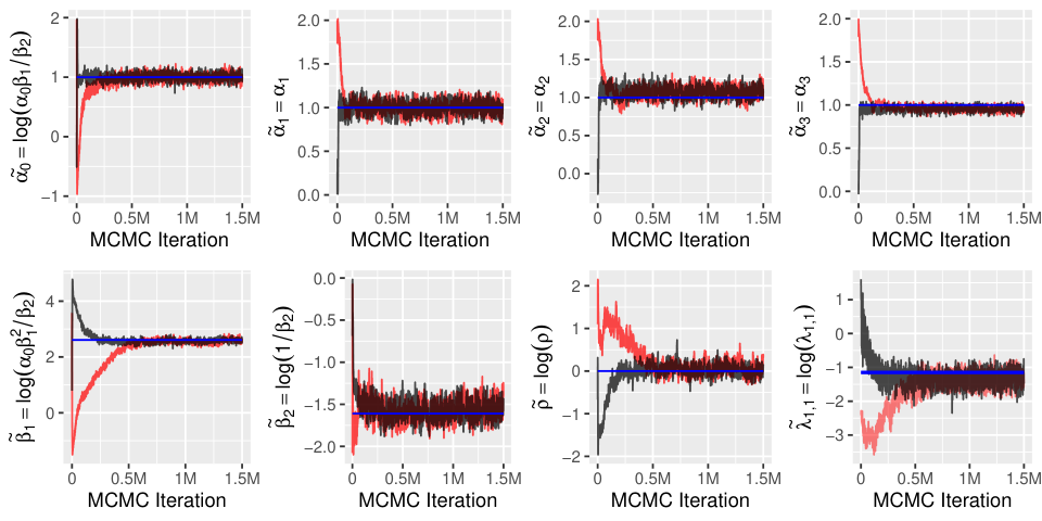
Figure 4 displays the trace plots for all the hyperparameters and one selected latent variable, for two MCMC chains with different initial values. The results show that there is good mixing and that convergence occurs very quickly for the regression parameters , , , and , and relatively quickly for the other hyperparameters or latent variables, despite the large number of latent variables. Essentially in this scenario, all Markov chains seem to have converged after about to iterations. For all parameters, the true value lies well within the corresponding posterior distribution, confirming the good performance of our algorithm. The effective sample size per minute is roughly between and , see Table 1 in the Supplementary Material. The proposal variances, automatically tuned in our algorithm, converged to the values for the hyperparameters (based on random walk proposals) and for the latent variables (based on MALA proposals). The total run time for each Markov chain is almost days to achieve million iterations.
We then study the ability of our model to predict values at unobserved locations. To this end, we treat the data at randomly selected sites as missing, and we compute the posterior predictive distributions at these sites. Figure 5 compares boxplots of the true simulated values at the prediction sites to posterior predictive samples obtained from fitting our model. Clearly, the posterior predictive distributions at all prediction sites appropriately capture the natural variability in the true data. This suggests that our algorithm succeeds in performing spatial prediction. The great benefit of our Bayesian approach is that estimation based on censored data and spatio-temporal prediction are performed simultaneously.
6 Application to precipitation extremes from Germany

6.1 Data description
We now study precipitation intensities observed in Germany, publicly available from the European Climate Assessment & Dataset project. The dataset reports daily precipitation amounts observed at more than spatial locations during the period 1941 to 2018. We apply our hierarchical models to a subset of locations with some missing data for the study period from 2009 to 2018. To avoid modeling complex seasonal non-stationarities, we consider the observations for the (full) months of September to December (i.e., for the extended autumn season), resulting in temporal replicates. This time period was merely selected based on temporal stationarity diagnostics, although from a practical perspective it would also be interesting in future research to extend our stationary models in order to study seasonal patterns in precipitation intensities during other months, as well as to assess the flood risk all year round. The site-specific mean precipitation intensities reported in Figure 6 show a tendency towards higher values in regions with higher altitudes; see Murawski et al. 2016 for more details about spatial and temporal trends in precipitation over Germany. In a preliminary analysis of the tail behavior of precipitation intensities, we fit the GP distribution to exceedances at each site separately with site-specific thresholds fixed at the empirical quantile of positive precipitation intensities. The maximum likelihood estimator, and the moment-based estimator of Dekkers et al. 1989 of the tail index, both provide systematically positive tail index estimates. This finding suggests that precipitation intensities are heavy-tailed as expected, and we proceed by fitting the spatial gamma-gamma model (3.2) to selected extreme precipitation events (see §6.3). The selection of extreme events and the modeling of their occurrences are described in §6.2.
6.2 Identifying and modeling extreme precipitation occurrences
The precipitation intensities are zero or very small for most of the days in the observation period, and we first extract extreme events (i.e., specific days) used to fit our spatial hierarchical model. Let denote the precipitation intensities at time and site , . To select extreme events, we consider the spatial average precipitation , indexed by time . We then define extreme events as days such that , where is the empirical cumulative distribution function of the sample of values. This scheme extracts extreme events in total.
Let denote the binary sequence of and values representing the occurrence indicators of extreme events for the -th year, with . That is, if the -th day of the year, with , was extreme in year , and otherwise. To capture temporal dependence, we model this time series through a logistic regression with a random effect defined as a first-order autoregressive Gaussian process, i.e.,
| (21) | ||||
with global intercept , autoregression coefficient , and marginal variance of , . We have explored a number of alternative models including an additional seasonal trend component in the regression equation (21), but we could not detect any significant improvement with respect to model (21).
We now present the estimation results for model (21). While there would be no notable obstacles for MCMC-based estimation of this model, we here propose using the integrated nested Laplace approximation (Rue et al. 2017, INLA,) implemented in the INLA package of the statistical software R. It provides fast and “off-the-shelf” Bayesian inference for logistic regression models such as (21). We obtain the following parameter estimates, with credible intervals in parentheses:
The estimated negative value of indicates that there is a higher probability for non-extreme events, as expected, while the estimated value of suggests that there is some non-negligible temporal persistence of zeros and ones. Figure 7 shows the fitted probability values for a selection of years (). The fitted models suggest relatively strong temporal autocorrelation: an extreme event at time entails an extreme event at time with probability substantially above average.
6.3 Modeling extreme precipitation intensities
We now return to the modeling of (non-zero) precipitation intensities, and we fit the gamma-gamma model (3.2) with latent Gaussian copula to the time series of selected extreme events. The model structure and data dimension are similar to those considered in the simulation study in §5. We use standardized latitude, longitude, and altitude as covariates in the model. The dataset of extreme events is composed of sites and days, leading to (spatially correlated) latent variables in the model. The minimum and maximum distances between the selected sites are km and km, receptively. We use sites for prediction and model validation (where the data are treated as completely missing). The remaining sites are used for model fitting. The proportion of missing observations at each of the training sites vary from to , for an average of . Our goal is also to compare how our model performs at different marginal thresholds, in order to assess the flexibility of our “sub-asymptotic” modeling approach, and we consider empirical quantiles at three moderately large probability levels, namely , and . Notice that while zero precipitation values may still occur at some spatial sites during extreme events, which creates a point mass at the lower endpoint of the precipitation distribution, we here avoid the tricky explicit treatment of zeros by censoring low precipitation intensities. We fit four different spatial models to the precipitation events obtained in §6.2, namely:
- D
-
Gamma-gamma model (3.2) with standardized spatial covariates given by latitude, longitude and altitude included in the scale parameter .
- D
-
Gamma-gamma model (3.2) with standardized spatial covariates given by latitude, longitude, and altitude included in both scale and shape parameters.
- D
-
Exponential-gamma (i.e., GP unconditionally) model, akin to Bopp and Shaby 2017, with standardized spatial covariates given by latitude, longitude, and altitude included in the scale parameter . This model may be obtained from Model D by fixing .
- D
-
Exponential-gamma (i.e., GP unconditionally) model, akin to Bopp and Shaby 2017, with standardized spatial covariates given by latitude, longitude, and altitude included in both scale and shape parameters. This model may be obtained from Model D by fixing .
We fit all four models using the MCMC algorithm detailed in §4. We chose random initial values for all the hyperparameters, while we used the copula structure of latent variables defined in (3.2) to generate initial values for the latent parameters. The trace plots displayed in Figure 8 show two MCMC chains with different initial values for all the hyperparameters and the latent parameter (site , day ) for model D with censoring threshold . The behavior of the chains for the other latent variables is similar to . The Markov chains for the other models (D, D, D) and for different censoring thresholds (, ) are similar to those displayed in Figure 8; see Figures , and in the Supplementary Material. The chains mix satisfactorily and converge to their stationary distribution after about – iterations for most parameters. Figure 7 in the Supplementary Material shows trace plots of the tuning parameters and for the MALA and random walk proposals, respectively. The tuning parameters stabilize well before the end of the first burn-in phase of iterations, which illustrates the good performance of our adaptive MCMC algorithm.
In Table 1, we compare models based on the continuous ranked probability score (CRPS) (Gneiting and Raftery 2007) and the tail weighted continuous ranked probability score (twCRPS) (Lerch et al. 2017) for all the models (D, D, D, and D) and for different censoring thresholds (, , and ). While the CRPS is a proper scoring rule widely used to assess calibration and sharpness of probabilistic forecasts, the twCRPS is similar but focuses on the largest fraction of the data only (i.e., the upper tail). Based on the CRPS, model D appears to be the best amongst the four models considered, with much better scores than the exponential-gamma models (D and D) and slightly better scores than the gamma-gamma model with covariates included both in the scale and the shape . However, based on the twCRPS, model D appears to be comparable to, yet still slightly better than model D. Since model D is more parsimonious and easier to fit, has only a slight difference in twCRPS compared to model D, and avoids issues of poor tail index predictions at unobserved sites (e.g., for unusual covariate values), we consider model D as our “best” model overall for our modeling extreme precipitation data over Germany. For brevity, we here only present the results for model D; see the Supplementary Material for more details on the other models.
| CRPS | twCRPS | |||||
|---|---|---|---|---|---|---|
| Model Threshold | ||||||
| D | 35.32 | 35.46 | 35.56 | 9.17 | 6.77 | 3.95 |
| D | 35.39 | 35.60 | 35.71 | 9.05 | 6.72 | 3.90 |
| D | 39.55 | 40.21 | 42.07 | 9.23 | 6.79 | 3.95 |
| D | 39.65 | 40.31 | 42.25 | 9.23 | 6.80 | 3.95 |
Table 2 reports posterior mean estimates and two-sided credible intervals for all hyperparameters and some latent parameters for model D. Interestingly, the results are fairly consistent across marginal censoring thresholds, indicating that our sub-asymptotic model can flexibly accommodate departure from the asymptotic GP distribution at finite levels; see also Figure 9, which compares boxplots of posterior predictive samples at all prediction sites for the three different censoring thresholds, , , and .
| Threshold | ||||||
|---|---|---|---|---|---|---|
| Parameter | Post. mean | CI | Post. Mean | CI | Post. Mean | CI |
As the conclusions are quite robust to the choice of the threshold, we now discuss the results for the threshold. The effect of the three covariates (latitude, longitude, altitude) is always significant as the credible intervals do not include . This result demonstrates the importance of including suitable geographical information in the scale parameter of the distribution. The estimates for latitude () and longitude () indicate that the south-western part of Germany receives higher precipitation amounts than the north-eastern part—a pattern that is clearly perceptible in the mean precipitation plot in left panel of Figure 6. Moreover, a clear positive effect of higher altitude on precipitation amounts arises with an estimate of (), which is also clear from the right panel of Figure 6. The estimate of the shape parameter is around and shows a huge difference with respect to the generalized Pareto model with . This finding substantiates our claim that extensions to the generalized Pareto distribution are useful for capturing complex data behavior at sub-asymptotic levels, and it confirms the comparison of models in Table 1. The estimated tail index at the censoring threshold is about , which corresponds to quite heavy tails. The estimated range parameter of the exponential correlation function is around km, implying a correlation of approximately at the latent level between two sites separated by km. This correlation decreases to approximately between the two furthest sites.
We now illustrate the spatial predictive performance of model D by QQ-plots and boxplots; see the Supplementary Material for diagnostics on the performance of the other models. To be concise, we here only discuss the results for the marginal censoring threshold ; see Figure 10. The results for the other marginal thresholds are similar and reported in the Supplementary Material. The first four rows in Figure 10 correspond to the prediction sites, which are treated as fully missing, and the last row displays QQ-plots for randomly chosen sites used for fitting the model. We use the prediction sites to assess whether our fitted model appropriately predicts marginal distributions at unobserved sites. The model quantiles displayed in these QQ-plots are based on the unconditional distribution, where , and are posterior mean estimates of , and for each site, respectively. We obtain uncertainty bands in the QQ-plots using a parametric bootstrap procedure accounting for missing values. Overall, the spatial predictive performance of model D is quite good, except perhaps at the prediction site 3, where our model tends to underestimate the empirical quantiles. Similar results were obtained for model D and other censoring levels with a generally satisfactory performance from low to high quantiles, but results are much worse for the exponential-gamma models D and D; see the Supplementary Material for details. Boxplots of posterior predictive distributions based on model D for all prediction sites (see Figure of the Supplementary Material), roughly correspond to the empirical distribution of the data available at these sites, though with a slightly larger variability as expected. This suggests that our model is able to adequately capture the natural variability of precipitation intensities at unobserved locations. Based on our graphical diagnostics, model D seems to be the best overall to predict the precipitation distribution at unobserved locations. Furthermore, our results illustrate how the spatial dependence structure assumed at the latent level in our model can help predict precipitation over space.
In summary, we conclude that our model appropriately captures spatial trends and dependence patterns of precipitation intensities during the extended autumn season in Germany. Specifically, it provides useful probabilistic predictions at unobserved locations during extreme events.
7 Conclusion
We have proposed several univariate models extending the generalized Pareto limit model for threshold exceedances, and studied their tail properties. The high flexibility of these models suggests that they are good candidates for threshold-based modeling of moderate to large values. Our models are based on hierarchical constructions using latent processes for spatial dependence. In this way, they avoid the artificial and overly strong separation of marginal and dependence modeling often encountered in spatial extreme value analysis.
Our Bayesian estimation approach bears witness of the power of the MALA for simulation-based estimation in cases where the dimension of the latent model is comparable to the number of observations. Its use with censored data for exceedance-based spatial extreme-value analysis allows bypassing high-dimensional numerical integration efficiently. Hence, our assumed model structure coupled with a data augmentation approach can be efficiently exploited to fit complex models in relatively high dimensions to censored threshold exceedances.
In our spatio-temporal precipitation data application, we have opted for a two-step modeling approach of extreme quantiles. Essentially, we first identify spatial extreme events, defined here as days with large spatially aggregated values at all locations, and then separately model their occurrences and intensities. More precisely, in the first step, we model the binary time series of occurrences (’s) or non-occurrences (’s) of spatial extreme events through logistic regression, and in the second step, we model the precipitation intensities of extreme events using a spatial hierarchical gamma-gamma model. This two-step approach has the benefit of reducing the number of latent variables included in our Bayesian model fitted in the second step, speeding up computations. Temporal dependence may be incorporated through covariate or random effect modeling in the logistic regression. In future research, it would be interesting to further extend the latent process of our spatial hierarchical model to take the spatio-temporal dependence of successive extreme precipitation intensities into account.
Acknowledgments
The data that support the findings of this study are openly available from the European Climate Assessment & Dataset project at https://www.ecad.eu/. This publication is based upon work supported by the King Abdullah University of Science and Technology (KAUST) Office of Sponsored Research (OSR) under Award No. OSR-CRG2017-3434.
References
- Andrieu and Thoms (2008) Andrieu, C. and Thoms, J. (2008) A tutorial on adaptive MCMC. Statistics and Computing 18, 343–373.
- Arendarczyk and Debicki (2011) Arendarczyk, M. and Debicki, K. (2011) Asymptotics of supremum distribution of a gaussian process over a weibullian time. Bernoulli 17(1), 194–210.
- Arneth et al. (2019) Arneth, A., Denton, F., Agus, F., Elbehri, A., Erb, K., Osman Elasha, B., Rahimi, M., Rounsevell, M., Spence, A. and Valentini, R. (2019) Framing and Context. In Climate Change and Land: an IPCC special report on climate change, desertification, land degradation, sustainable land management, food security, and greenhouse gas fluxes in terrestrial ecosystems, eds P. Shukla, J. Skea, E. C. Buendia, V. Masson-Delmotte, H.-O. Pörtner, D. Roberts, P. Zhai, R. Slade, S. Connors, R. van Diemen, M. Ferrat, E. Haughey, S. Luz, S. Neogi, M. Pathak, J. Petzold, J. P. Pereira, P. Vyas, E. Huntley, K. Kissick, M. Belkacemi and J. Malley. In press.
- Bacro et al. (2020) Bacro, J.-N., Gaetan, C., Opitz, T. and Toulemonde, G. (2020) Hierarchical space-time modeling of asymptotically independent exceedances with an application to precipitation data. Journal of the American Statistical Association. 115, 555–569.
- Banerjee et al. (2014) Banerjee, S., Carlin, B. P. and Gelfand, A. E. (2014) Hierarchical modeling and analysis for spatial data. Second edition. CRC Press.
- Bopp and Shaby (2017) Bopp, G. P. and Shaby, B. A. (2017) An exponential–gamma mixture model for extreme Santa Ana winds. Environmetrics 28, e2476.
- Bortot and Gaetan (2014) Bortot, P. and Gaetan, C. (2014) A Latent Process Model for Temporal Extremes. Scandinavian Journal of Statistics 41(3), 606–621.
- Bortot and Gaetan (2016) Bortot, P. and Gaetan, C. (2016) Latent process modelling of threshold exceedances in hourly rainfall series. Journal of Agricultural, Biological and Environmental Statistics 21(3), 531–547.
- Breiman (1965) Breiman, L. (1965) On some limit theorems similar to the arc-sin law. Theory of Probability & Its Applications 10(2), 323–331.
- Carreau and Bengio (2009) Carreau, J. and Bengio, Y. (2009) A hybrid Pareto model for asymmetric fat-tailed data: the univariate case. Extremes 12(1), 53–76.
- Castro-Camilo and Huser (2019) Castro-Camilo, D. and Huser, R. (2019) Local likelihood estimation of complex tail dependence structures, applied to U.S. precipitation extremes. Journal of the American Statistical Association 115, 1037–1054.
- Castro-Camilo et al. (2019) Castro-Camilo, D., Huser, R. and Rue, H. (2019) A spliced Gamma-generalized Pareto model for short-term extreme wind speed probabilistic forecasting. Journal of Agricultural, Biological and Environmental Statistics 24, 517–534.
- Cooley et al. (2007) Cooley, D., Nychka, D. and Naveau, P. (2007) Bayesian spatial modeling of extreme precipitation return levels. Journal of the American Statistical Association 102(479), 824–840.
- Cressie (1993) Cressie, N. A. C. (1993) Statistics for spatial data. Wiley Online Library.
- Davison and Gholamrezaee (2012) Davison, A. C. and Gholamrezaee, M. M. (2012) Geostatistics of extremes. Proceedings of the Royal Society A: Mathematical, Physical & Engineering Sciences 468(2138), 581–608.
- Davison and Huser (2015) Davison, A. C. and Huser, R. (2015) Statistics of Extremes. Annual Review of Statistics and its Application 2, 203–235.
- Davison et al. (2019) Davison, A. C., Huser, R. and Thibaud, E. (2019) Spatial extremes. In Handbook of Environmental and Ecological Statistics, eds A. E. Gelfand, M. Fuentes, J. A. Hoeting and R. L. Smith. Boca Raton: CRC press.
- Davison et al. (2012) Davison, A. C., Padoan, S. and Ribatet, M. (2012) Statistical modelling of spatial extremes (with Discussion). Statistical Science 27(2), 161–186.
- Davison and Smith (1990) Davison, A. C. and Smith, R. L. (1990) Models for exceedances over high thresholds (with discussion). Journal of the Royal Statistical Society: Series B (Statistical Methodology) 52(3), 393–442.
- de Fondeville and Davison (2018) de Fondeville, R. and Davison, A. C. (2018) High-dimensional peaks-over-threshold inference. Biometrika 105(3), 575–592.
- Dekkers et al. (1989) Dekkers, A. L., Einmahl, J. H., De Haan, L. et al. (1989) A moment estimator for the index of an extreme-value distribution. The Annals of Statistics 17(4), 1833–1855.
- Eastoe and Tawn (2009) Eastoe, E. F. and Tawn, J. A. (2009) Modelling non-stationary extremes with application to surface level ozone. Journal of the Royal Statistical Society: Series C (Applied Statistics) 58(1), 25–45.
- Fougeres and Mercadier (2012) Fougeres, A.-L. and Mercadier, C. (2012) Risk measures and multivariate extensions of Breiman’s theorem. Journal of Applied Probability 49(2), 364–384.
- Frigessi et al. (2003) Frigessi, A., Haug, O. and Rue, H. (2003) A dynamic mixture model for unsupervised tail estimation without threshold selection. Extremes 5(3), 219–235.
- Gneiting and Raftery (2007) Gneiting, T. and Raftery, A. E. (2007) Strictly proper scoring rules, prediction, and estimation. Journal of the American statistical Association 102(477), 359–378.
- Huser and Davison (2014) Huser, R. and Davison, A. C. (2014) Space-time modelling of extreme events. Journal of the Royal Statistical Society: Series B (Statistical Methodology) 76(2), 439–461.
- Huser et al. (2017) Huser, R., Opitz, T. and Thibaud, E. (2017) Bridging asymptotic independence and dependence in spatial extremes using Gaussian scale mixtures. Spatial Statistics 21, 166–186.
- Huser and Wadsworth (2019) Huser, R. and Wadsworth, J. L. (2019) Modeling spatial processes with unknown extremal dependence class. Journal of the American Statistical Association 114, 434–444.
- Lerch et al. (2017) Lerch, S., Thorarinsdottir, T. L., Ravazzolo, F., Gneiting, T. et al. (2017) Forecaster’s dilemma: Extreme events and forecast evaluation. Statistical Science 32(1), 106–127.
- Murawski et al. (2016) Murawski, A., Zimmer, J. and Merz, B. (2016) High spatial and temporal organization of changes in precipitation over Germany for 1951–2006. International Journal of Climatology 36, 2582–2597.
- Naveau et al. (2016) Naveau, P., Huser, R., Ribereau, P. and Hannart, A. (2016) Modeling jointly low, moderate, and heavy rainfall intensities without a threshold selection. Water Resources Research 52(4), 2753–2769.
- Opitz et al. (2018) Opitz, T., Huser, R., Bakka, H. and Rue, H. (2018) INLA goes extreme: Bayesian tail regression for the estimation of high spatio-temporal quantiles. Extremes 21(3), 441–462.
- Papastathopoulos and Tawn (2013) Papastathopoulos, I. and Tawn, J. A. (2013) Extended generalised Pareto models for tail estimation. Journal of Statistical Planning and Inference 143(1), 131–143.
- Power and Delage (2019) Power, S. B. and Delage, F. c. P. D. (2019) Setting and smashing extreme temperature records over the coming century. Nature Climate Change 9, 529–534.
- Reiss and Thomas (2007) Reiss, R.-D. and Thomas, M. (2007) Statistical Analysis of Extreme Values. Third edition. Basel: Birkhäuser.
- Resnick (1987) Resnick, S. I. (1987) Extreme values, regular variation and point processes. Springer.
- Risser and Wehner (2017) Risser, M. D. and Wehner, M. F. (2017) Attributable human-induced changes in the likelihood and magnitude of the observed extreme precipitation during Hurricane Harvey. Geophysical Research Letters 44(24), 12457–12464.
- Roberts and Rosenthal (1998) Roberts, G. O. and Rosenthal, J. S. (1998) Optimal scaling of discrete approximations to langevin diffusions. Journal of the Royal Statistical Society: Series B (Statistical Methodology) 60(1), 255–268.
- Roberts and Tweedie (1996) Roberts, G. O. and Tweedie, R. L. (1996) Exponential convergence of Langevin distributions and their discrete approximations. Bernoulli 2(4), 341–363.
- Rue et al. (2017) Rue, H., Riebler, A., Sørbye, S. H., Illian, J. B., Simpson, D. P. and Lindgren, F. K. (2017) Bayesian computing with inla: a review. Annual Review of Statistics and Its Application 4, 395–421.
- Scarrott and MacDonald (2012) Scarrott, C. and MacDonald, A. (2012) A Review of Extreme Value Threshold Estimation And Uncertainty Quantification. REVSTAT 10(1), 33–60.
- Simpson et al. (2017) Simpson, D. P., Rue, H., Riebler, A., Martins, T. G. and Sørbye, S. H. (2017) Penalising model component complexity: A principled, practical approach to constructing priors. Statistical Science 32(1), 1–28.
- Stein (2020a) Stein, M. L. (2020a) Parametric models for distributions when interest is in extremes with an application to daily temperature. Extremes To appear.
- Stein (2020b) Stein, M. L. (2020b) A parametric model for distributions with flexible behavior in both tails. Environmetrics To appear.
- Vettori et al. (2019) Vettori, S., Huser, R. and Genton, M. G. (2019) Bayesian modeling of air pollution extremes using nested multivariate max-stable processes. Biometrics 75, 831–841.
- Vettori et al. (2020) Vettori, S., Huser, R., Segers, J. and Genton, M. G. (2020) Bayesian model averaging over tree-based dependence structures for multivariate extremes. Journal of Computational and Graphical Statistics 29, 174–190.
- Wadsworth and Tawn (2014) Wadsworth, J. L. and Tawn, J. A. (2014) Efficient inference for spatial extreme value processes associated to log-Gaussian random functions. Biometrika 101(1), 1–15.
- Witze (2018) Witze, A. (2018) Why extreme rains are gaining strength as the climate warms. Nature 563(7732), 458–460.