MaskAAE: Latent space optimization for Adversarial Auto-EncodersThanks: . work done when at IIT Delhi

In this section, we theoretically examine the effect of latent dimensionality on the quality of generated data in AE based generative models. We show that if dimensionality of the latent space $\mathcal{Z}$ is more than the optimal dimensionality (to be defined), $\Pi({\bm{z}})$ and $\Psi({\bm{z}})$ diverge too much whereas it being less leads to information loss.

To start with, we allow a certain inductive bias in assuming that nature generates the data as described in Figure 2 using the following two-step process: First sample from some isotropic continuous latent distribution in $n$-dimensions (call this $\widetilde{\Psi}$ over $\widetilde{\mathcal{Z}}$), and then pass this through a function $f:\displaystyle\mathbb{R}^{n}\to\displaystyle\mathbb{R}^{d}$, where $d$ is the dataset dimensionality. Typically $d>>n$, thereby making data to lie on a low-dimensional manifold in $R^{d}$. Since $\widetilde{\mathcal{Z}}$ can intuitively be viewed as the latent space from which the nature is generating the data, we call $n$ the true latent dimension and function $f$, as the data-generating function. Note that within this ambit, $\widetilde{\mathcal{Z}}$ forms the domain of $f$ and it is unique only up to its range with the following properties:

1. A1

   $f$ is $L$-lipschitz: $\exists$ some finite $L\in\displaystyle\mathbb{R}^{+}$ satisfying $||f(\widetilde{\bm{z}}_{1})-f(\widetilde{\bm{z}}_{2})||\leq L||\widetilde{\bm{z}}_{1}-\widetilde{\bm{z}}_{2}||,\,\,\forall\widetilde{\bm{z}}_{1},\widetilde{\bm{z}}_{2}\in\widetilde{\mathcal{Z}}$.

2. A2

   There does not exist $f^{*}:\displaystyle\mathbb{R}^{n^{\prime}}\to\displaystyle\mathbb{R}^{d},n^{\prime}<n$ satisfying A1 such that the range of $f$ is a subset of the range of $f^{*}$.

The first property is satisfied by a large class of functions, including neural networks and the second simply states that $n$, the dimension of the domain (generative latent space) of $f$ is minimal¹¹ 1 If there exists such an $f^{*}$, then that would become the generating function with $n^{\prime}$ being minimal.. Hence, it is reasonable to impose these restrictions on data-generating functions. (An illustrative example is provided in the supplementary material.)

In this section, we formulate the conditions required for faithful generation in latent variable generative models. Let $\Gamma({\bm{x}},{\bm{z}})$ and $\Gamma^{\prime}({\bm{x}},{\bm{z}})$ denote the true and the (implicitly) inferred joint distribution of the observed and latent variables. The goal of latent variable generative models is to minimize the negative log-likelihood of $\Gamma^{\prime}({\bm{x}},{\bm{z}})$ under $\Gamma({\bm{x}},{\bm{z}})$:

An AE-based generative model would attempt to minimize Eq. 1 by learning two parametric functions, $E_{\kappa}\triangleq g:\displaystyle\mathbb{R}^{d}\to\displaystyle\mathbb{R}^{m}$ ($m$ is hereafter referred to as assumed latent dimension / model capacity) and $D_{\psi}\triangleq g^{\prime}:\displaystyle\mathbb{R}^{m}\to\displaystyle\mathbb{R}^{d}$, to approximate the distributions $\Psi({\bm{z}}|{\bm{x}})$ and $\Gamma({\bm{x}}|{\bm{z}})$, respectively. Further, Eq. 1 can be broken down into two terms, and the objective of any AE based model can be restated as:

If $E_{\kappa}$ and $D_{\psi}$ are deterministic (as in the case of AAE (Makhzani et al. 2016), WAE (Zhang et al. 2019) etc.), then the two terms in Eq. 2 can be cast as the following two requirements (see the supplement for the proof):

1. R1

   $f(\widetilde{\bm{z}})=g^{\prime}(g(f(\widetilde{\bm{z}})))\;\forall\ \widetilde{\bm{z}}\ \in\displaystyle\mathbb{R}^{n}$. This condition states that the reconstruction error between the real and generated data should be minimal.

2. R2

   The Cross Entropy $\mathcal{H}(\Psi,\Pi)$ between the chosen prior $\Psi$, and $\Pi$ on $\mathcal{Z}$ is minimal.

With this, we state and prove the conditions required to ensure R1 and R2 are met with assumed data generation process.

Proof: We prove by contradicting either R1 or R2, in assuming both the cases of $m<n$ or $m>n$.

Case A $(m<n)$: For R1 to hold, the range of $f$ must be a subset of the range of $g^{\prime}$. Further, since $g^{\prime}$ is a Neural Network, it satisfies A1. But, by A2, such a function cannot exist if $m<n$.
Case B $(m>n)$: For the sake of simplicity, let us assume that $\widetilde{\mathcal{Z}}$ is a unit cube²² 2 One can easily obtain another function $\nu:[0,1]^{n}\to\widetilde{\mathcal{Z}}$ that scales and translates the unit cube appropriately. Note that for such a $\nu$ to exist, we need $\widetilde{\mathcal{Z}}$ to be bounded, which may not be the case for certain distributions like the Gaussian distributions. Such distributions, however, can be approximated successively in the limiting sense by truncating at some large value Rudin et al. 1964 in $\displaystyle\mathbb{R}^{n}$. We show in Lemma 2 and 3 that in this case, R2 will be contradicted if $m>n$. The idea is to first show that the range of $g\circ f$ will have Lebesgue measure 0 (Lemma 1) and this leads to arbitrarily large $\mathcal{H}$ (Lemma 2).
Lemma 1: Let $\Omega:[0,1]^{\alpha}\to\displaystyle\mathbb{R}^{\beta}$ be an $L-lipschitz$ function. Then its range $R\in\displaystyle\mathbb{R}^{\beta}$ has Lebesgue measure $0$ in $\displaystyle\mathbb{R}^{\beta}$ dimensions if $\beta>\alpha$.

Proof:

For some $\epsilon\in\mathbb{N}$, consider the set of points:

S={$(\frac{a_{0}+0.5}{\epsilon},\ldots,\frac{a_{\alpha-1}+0.5}{\epsilon})\big|a_{i}\in\{0,\ldots,\epsilon-1\}$}.
Construct closed balls around them having radius $\frac{\sqrt{\alpha}}{2\epsilon}$. It is easy to see that every point in the domain of $\Omega$ is contained in at least one of these balls. This is because, for any given point, the nearest point in S can be at-most $\frac{1}{2\epsilon}$ units away along each dimension. Also, since $\Omega$ is $L$-lipschitz, we can conclude that the image set of a closed ball having radius $r$ and centre ${\bm{u}}\in[0,1]^{\alpha}$ would be a subset of the closed ball having centre $\Omega({\bm{u}})$ and radius $L\times r$.
The range of $\Omega$ is then a subset of the union of the image sets off all the closed balls defined around S. The volume of this set is upper bounded by the sum of the volumes of the individual image balls, each having volume $\frac{c}{\epsilon^{\beta}}$ where c is a constant having value $\frac{(L)^{\beta}(\alpha\pi)^{\frac{\beta}{2}}}{\Gamma(\frac{\beta}{2}+1)}$. Therefore,

The final quantity of Eq. 3 can be made arbitrarily small by choosing $\epsilon$ appropriately. Since the Lebesgue measure of a closed ball is same as its volume, the range of $\Omega$, $R$ has measure $0$ in $\displaystyle\mathbb{R}^{\beta}.$∎
Since $f,\text{ and }g$ are Lipschitz, $g\circ f$ must have a range with Lebesgue measure 0 as a consequence of Lemma 2. Now we show that as a consequence of the range of $g\circ f$ (call it $\mathcal{R}$) having measure $0$, the cross-entropy between $\Pi$ and $\Psi$ goes to

infinity.
Lemma 2: If $\Pi$ and $\Psi$ are two distributions as defined in Sec.3.1 such that the support of the latter has a $0$ Lebesgue measure, then $\mathcal{H}(\Pi,\Psi)$ grows to be arbitrarily large.
Proof: $\Psi$ can be equivalently expressed as:

Define $\mathbb{I}_{\mathcal{R}}$ as the indicator function of $\mathcal{R}$, i.e.

Since $\mathcal{R}$ has measure $0$ (Lemma 2), we have

Further, since $\mathbb{I}_{\mathcal{R}}$ is identically $1$ in the support of $\Psi$, we have

Now consider the cross-entropy between $\Pi$ and $\Psi$ given by:

for any arbitrarily large positive real $\varrho$. This holds true because $\mathbb{I}_{\mathcal{R}}$ is identically 0 over the domain of integration. Further,

Combining 8 and 9, the required cross-entropy is lower bounded by an arbitrarily large quantity $\varrho$.∎
Thus Lemma 2 contradicts R2 required for good generation when $m>n$. Therefore, to ensure good generation neither $m>n$ nor $m<n$ can be true. Thus, the only possibility is $m=n$. This concludes Theorem 1.∎


One can ensure good generation, by satisfying both R1 and R2 via a trivial solution in the form of $g^{\prime}=f$ with an appropriate $g$ and making $m=n$. However, since neither $n$ nor $f$ is known, one needs a practical method to ensure $m$ to approach $n$ which is described in the next section.

Our premise in section 3.2 demands a pair of deterministic Encoder and Decoder networks satisfying R1 and R2, to ensure good quality generation. AE-models with deterministic $E_{\kappa}$ and $D_{\psi}$ networks, such as Adversarial Auto-Encoder (AAE) (Makhzani et al. 2016) and Wasserstein Auto-Encoder (WAE) (Zhang et al. 2019) implement R1 by approximating norm-based losses and R2 through an adversarial training mechanism under metrics such as JS-Divergence or Wasserstein distance. However, most of the time, the choice of the latent dimensionality is ad hoc and there is no mechanism to get rid of the excess latent dimensions that is critical for good-quality generation as demanded by Theorem 1. Therefore, in this section, we take the ideas presented in Section 3, and propose an architectural modification on models such as AAE/WAE, such that being initialized with a large enough estimated latent space dimension the model would learn a binary-mask automatically discovering the right number of latent dimensions required.

Specifically, we propose the following modifications in the AAE-like architecture (Makhzani et al. 2016; Zhang et al. 2019), which contain an additional component called Discriminator ($H_{\zeta}$ ) that is used to match $\Psi({\bm{z}})$ and $\Pi({\bm{z}})$ via adversarial learning. Our model, called the MaskAAE is detailed in figure 3.

1. 1.

   We introduce a trainable mask layer, $\mu\in\{0,1\}^{m}$, just after the final layer of the Encoder network.

2. 2.

   Before passing the encoded representation, $\hat{\bm{z}}$ of an input image ${\bm{x}}$ to the decoder network ($D_{\psi}$ ) and the Discriminator network ($H_{\zeta}$ ) a Hadamard product is performed between $\hat{\bm{z}}$ and $\mu$.

3. 3.

   A Hadamard product is performed between the prior sample, ${\bm{z}}\sim\Pi({\bm{z}})$ and the same mask $\mu$ as in item (1), before passing it as an input to the discriminator network $H_{\zeta}$ to ensure R2.

4. 4.

   During inference, the prior samples are multiplied with the learned mask before giving as input to the Decoder ($D_{\psi}$ ) network which serves the generator.

Intuitively, masking of both the encoded latent vector and prior with a same binary mask allows us to work only with a subset of dimensions in the latent space. This means that even though $m$ (the initial assumed latent dimensionality) may be greater than $n$, mask (if learned properly) reduces the encoded latent space to $\mathcal{R}^{n}$. This will in-turn facilitate better matching of $\Psi({\bm{z}})$ and $\Pi({\bm{z}})$ (R2) required for better generation.

MaskAAE is trained exactly similarly as one would train an AAE/WAE but with the addition of a loss term to train the mask layer. Here, we provide the details of the mask-loss only. For a complete description of other AAE/WAE based training loss terms refer to the supplementary material.

Although, the mask by definition is a binary-valued vector, to facilitate gradient flow during training, we relax it to be continuous valued while penalizing it for deviation from either $0$ or $1$. Specifically, we parameterize $\mu$ using a vector $\theta\in\displaystyle\mathbb{R}^{m}$ such that $\mu=b(\theta)$ where, $b(\theta)=\max(0,1-e^{-\theta})$. $\theta$ is initialized by drawing samples from $\mathcal{U}[0,a]$, where $a\in\mathbb{Z}^{+}$. Intuitively, this parameterization bounds $\mu$ in the range $(0,1)$. Since the mask layer affects both the requirements R1 and R2, it is trained so as to minimize both the norm-based reconstruction error (first term in Eq. 10) and divergence metrics such as JS-divergence or Wasserstein’s distance, between the masked prior distribution and the masked encoded latent distribution (second term in Eq. 10). Finally, a polynomial regularizer (third term in Eq. 10) is also added on $\mu$ so that any deviation from $\{0,1\}$ is penalized. Therefore, the final objective function for the mask layer, $L_{mask}$ consists of three terms as below.

where, $\omega=\frac{1}{s}\sum_{i}H_{\zeta}(\mu\odot{\bm{z}}^{(i)})-\frac{1}{s}\sum_{i}H_{\zeta}(\mu\odot E_{\kappa}({\bm{x}}^{(i)}))$ is the Wasserstein’s distance, $s$ denotes batch size, and the weights $(\lambda_{1}$, $\lambda_{2}$, $\lambda_{3})$ of different loss terms are hyper-parameters. Details about the training algorithm, and the architectures for $E_{\kappa}$ , $D_{\psi}$ and $H_{\zeta}$ are available in the supplementary material.

In the following description, we will use $n$ to denote the true latent dimension, and $m$ to denote the assumed latent dimension (or model capacity) in line with the notation used earlier in the paper. Assuming that data is generated according to the generation process described in Section 3, we are interested in answering the following questions: (a) Given sufficient model capacity (i.e, $m\geq n$ and sufficiently powerful $E_{\kappa}$, $D_{\psi}$ and $H_{\zeta}$), can MAAE discover the true number of latent dimensions? (b) What is the quality of the data generated by MAAE for varying values of $m$?

In an ideal scenario, we would expect that whenever $m\geq n$, MAAE masks $(m-n)$ number of dimensions. Further, we would expect that the performance of MAAE is independent of the value of $m$, whenever $m\geq n$. For each value of $m$ that we experimented with, we also trained an equivalent WAE model with exactly the same architecture for $E_{\kappa}$ , $D_{\psi}$ and $H_{\zeta}$ as in MAAE without the mask layer. We would expect the performance of the WAE model to deteriorate in cases whenever $m<n$ or $m>n$ if our theory were to hold correct.

In line with our assumed data generation process, the data for our synthetic experiments is generated using the following process.

• •

  Sample $\tilde{{\bm{z}}}\sim\mathcal{N}(\mu_{s},\Sigma_{s})$, where the mean $\mu_{s}\in\displaystyle\mathbb{R}^{n}$ was fixed to be zero and $\Sigma_{s}\in\displaystyle\mathbb{R}^{n\times n}$ represents the diagonal co-variance matrix (isotropic Gaussian).

• •

  Compute ${\bm{x}}=f(\tilde{{\bm{z}}})$, where $f$ is a non-linear function computed using a two-layer fully connected neural network with $k$ units in each layer, $d>>n$ output units, and using leaky ReLU as the non-linearity (refer to the supplement for more details). The weights of these networks are randomly fixed and $k$ was taken as 128.

We set $n=8$ and $16$, and varied $m$ in the range of $[2,32]$ and $[2,78]$ with step size $2$, for $n=8$ and $n=16$ respectively. We use the standard Fréchet Inception Distance (FID) (Heusel et al. 2017) score between generated and real images to validate the quality of the generated data, because FID has been shown to correlate well the human visual perception and also sensitive to artifacts such as mode collapse (Lucic et al. 2018; Sajjadi et al. 2018). Figure 4 (a) and (b) presents our results on synthetic data. On X-axis, we plot $m$ and Y-axis (left) plots the FID score comparing MAAE and WAE for different values of $m$. Y-axis (right) plots the number of active dimensions discovered by our algorithm. It is seen that both MAAE and WAE, achieve the best FID score when $m=n$. But whereas the performance for WAE deteriorates with increasing $m$, MAAE retains the optimal FID score independent of the value of $m$. Further, in each case, we get very close to the true number of latent dimensions, even with different values of $m$ (as long as $m>8$ or $16$, respectively). This clearly validates our theoretical claims, and also the fact that MAAE is capable of offering good quality generation in practice.

In this section, we examine the behavior of MAAE on real-world datasets. In this case, the true latent data dimensions ($n$) is unknown, but we can still analyze the behavior as the estimated latent number of dimension ($m$) is varied. We work on four image datasets used extensively in the literature: (a) MNIST (Lecun 2010) (b) Fashion MNIST (Xiao et al. 2017) (c) CIFAR-10 (Krizhevsky 2009) (d) CelebA (Liu et al. 2015) with standard test/train splits.

In our first set of experiments, we perform an analysis similar to the one done in the case of synthetic data, for the MNIST dataset. Specifically, we varied the estimated latent dimension (model capacity $m$) for MNIST from $10$ to $110$, and analyzed the FID score, as well as the true dimensionality as discovered by the model. For comparison, we also did the same experiment using the WAE model. Figure 4 (c) shows the results. As in the case of synthetic data, we observe a U-shape behavior for the WAE model, with the lowest value achieved at $m=13$. This validates our thesis that the best performance is achieved at a specific value of latent dimension, which is around $13$ in this case. Further, looking at MAAE curve, we notice that the performance (FID score) more or less stabilizes for values of $m\geq 10$. In addition, the true latent dimension discovered also stabilizes around $10-13$ irrespective of $m$, without compromising much on the generation quality. Note that the same network architecture was used at all points of Figure 4. These observations are in line with the expected behavior of our model, and the fact that our model can indeed mask the spurious set of dimensions to achieve good generation quality.

Figure 5 shows the behaviour of mask for model capacity $m=32,64$ and $110$ on MNIST dataset. Interestingly, in each case, we are able to discover almost the same number of unmasked dimensions, independent of the starting point. It is also observed that the Wasserstein distance is minimized at the point where the mask reaches the optimal point (Refer to supplementary material for the plots).

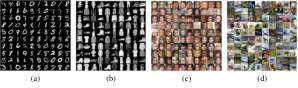
Finally, to measure generation quality, we present the FID scores of our method in Table 1 along with several state-of-the-art AE-based models mentioned in section 2. Our approach achieves the best FID score on all the datasets compared to the state-of-the-art AE based generative models. Performance of MAAE is also comparable to that of GANs listed in Lucic et al. 2018, despite using a simple norm based reconstruction loss and an isotropic uni-modal Gaussian prior. Figure 6 presents some randomly generated samples by our algorithm for each of the datasets.

The better FID scores of MAAE can be attributed to better distribution matching in the latent space between $\Psi({\bm{z}})$ and $\Pi({\bm{z}})$. But quantitatively comparing the matching between the two distributions is not easy as MAAE might mask out some of the latent dimensions resulting in a mismatch between the dimensionality of latent space in different models, thus rendering the usual metrics not suitable. We therefore calculate the averaged off-diagonal normalized absolute co-variance⁴⁴ 4 Refer supplementary material for mathematical formula. (NAC) of the encoded latent vectors and report it in Table 2 (Refer supplementary material for the full Co-variance matrix). Since $\Pi({\bm{z}})$ is assumed to be an isotropic Gaussian, ideally NAC should be zero and any deviation from zero indicates a mismatch. For MAAE we use only the unmasked latent dimensions for the NAC calculation, this is to ensure that NAC is not underestimated by considering the unused dimension. It is observed that for the same model capacity, MAAE has lesser NAC than the corresponding WAE indicating better distribution matching in the latent space.

These results clearly demonstrate that not only MAAE can achieve the best FID scores on a number of benchmarks datasets, it also serves as a first step in discovering the underlying latent structure for a given dataset. To the best of our knowledge, this is the first study analyzing (and discovering) the effect of latent dimensions on the generation quality.

In the main paper, we have stated the following conditions as requirements for optimal generation:

1. R1

   $f(\widetilde{\bm{z}})=g^{\prime}(g(f(\widetilde{\bm{z}})))\;\forall\ \widetilde{\bm{z}}\ \in\displaystyle\mathbb{R}^{n}$.

2. R2

   $\mathcal{H}(\Psi,\Pi)$ on $\mathcal{Z}$ is minimal.

In this section, we shall show that these are indeed necessary and sufficient to minimise the cross-entropy between the true data distribution $\Gamma$ and the generated data distribution $\Gamma^{\prime}$.
Since auto-encoder based frameworks work through a latent space $\mathcal{Z}$, their objective is to minimise the cross entropy between the joint distribution of ${\bm{x}}$ and ${\bm{z}}$. We define these joint distributions as:

where $\delta$ is the Dirac delta function. The cross entropy between these two distributions can be broken down as follows:

The first term in the final expression can further be expressed as:

If the equality inside the delta function does not hold at any point, it will push the logarithm to negative infinity, and in turn the entire quantity will become very high. To prevent this, we need ${\bm{x}}=g^{\prime}(g({\bm{x}}))$ at all points. Since ${\bm{x}}$ varies over the range of $f$, this reduces to R1.
In the second term, the expectation is over a joint distribution, but the variable ${\bm{x}}$ never appears inside the expectation, so it is safe to take the expectation over the marginal of ${\bm{z}}$. However, this marginal, $\Gamma({\bm{z}})$ is exactly the distribution imposed on the latent space by the encoder and the data distribution, which we previously called $\Psi$. Making this change turns this term into $\mathcal{H}(\Psi,\Pi)$ and since we need this to be minimal, we recover the R2.

Our generative process assumes that $n$, the dimension of the input space of $f$ is minimal. Intuitively this means that each of the latent dimension contributes in generation of some (possibly small) region in the domain of the observed data but it is not necessary that every latent dimension (independently) affects every observed data point.

For example, consider the case where a leaf is being photographed. A young leaf in broad daylight has colour roughly (120,100,50) in the HSL system. As the age of the leaf increases, the lightness starts to fall, but a similar fall in lightness will also be observed with fading daylight. At this point, lighting conditions and age of leaf have identical effect on the appearance of the leaf. However, after a point, age will start reducing the hue of the leaf, while lighting conditions will continue decreasing its lightness. Since at this point these two factors influence the outcome differently, they can be separate factors in our input space. On the other hand, the distance from which the photo was taken and the optical zoom of the lens will always have similar effect, and therefore, only one of these is allowed as a factor. Note that this example is presented for illustrative purposes only, and in real cases, the input factors are unlikely to directly map to real-world causes.

In the main paper, we have claimed that given a set $S$, defined as: $S$={$(\frac{a_{0}+0.5}{\epsilon},\ldots,\frac{a_{n-1}+0.5}{\epsilon})\big|a_{i}\in\{0,\ldots,\epsilon-1\}$} if we build closed balls around each point in $S$, then every point in $[0,1]^{n}$ lies in atleast one of these balls. To further the intuition behind this, we present an illustration for the case where $n=2$ and $\epsilon=4$.

In figure 7 the big square represents the unit square. By the nature of Cartesian space, this can be tiled completely by 64 smaller squares having side $\frac{1}{8}$ units. The 16 circles represent the closed balls in $\mathbb{R}^{2}$. It is easy to see that each of the smaller squares lies completely in some circle. Since each point in the bigger square must lie in one of the smaller squares, they also lie in one of the circles.

Next, corresponding to each of the components above, we present a loss function where $s$ represents the batch size.

1. 1.

   Auto-Encoder Loss: This is the standard loss to capture the quality of re-construction as used earlier in the AE literature. In addition, we have a term corresponding to minimization of the variance over the masked dimensions in the encoded output in a batch. The intuition is that encoder should not inject information into the dimensions which are going to be masked anyway. The loss is specified as:

   $$\begin{split}L_{ae}&=\frac{\alpha_{1}}{s}\sum_{i=1}^{s}||{\bm{x}}^{(i)}-D_{\psi}(\mu\odot E_{\kappa}({\bm{x}}^{(i)}))||\\ &\qquad+\alpha_{2}(\delta^{T}Diag(A))\end{split}$$

   (14)

   $A$ represents the co-variance matrix for the encoding matrix $E_{\kappa}(X)$, $X$ being the data matrix for the current batch. $\delta$ is the vector obtained by applying the function $a(u)=e^{-\gamma\times u}$ point-wise to $\mu$. $\alpha_{1}$, $\alpha_{2}$ and $\gamma$ are hyperparameters.

2. 2.

   Generator Loss: This is the loss capturing the quality of generation in terms of how far the generated distribution is from the prior distribution. This loss measures the ability of the encoder to generate the samples such that they are coming from $\Pi({\textnormal{z}})$ which is ensured using the generator loss mentioned in Arjovsky et al. 2017:

   $$L_{gen}=-\frac{1}{s}\sum_{i=1}^{s}H_{\zeta}(\mu\odot E_{\kappa}({\bm{x}}^{(i)}))$$

   (15)

3. 3.

   Distribution-Matching Loss: This is the loss incurred by the Distribution-matching network, $H_{\zeta}$ in matching the distributions. We use Wasserstein’s distance (Arjovsky et al. 2017) to measure the distributional closeness with the following loss:

   $$\begin{split}L_{dm}&=-\frac{1}{s}\sum_{i=1}^{s}H_{\zeta}(\mu\odot{\bm{z}}^{(i)})+\frac{1}{s}\sum_{i=1}^{s}H_{\zeta}(\mu\odot\hat{{\bm{z}}}^{(i)})\\ &\qquad+\frac{\beta_{2}}{s}\sum_{i=1}^{s}\big(\lvert\lvert\nabla_{{\bm{z}}_{avg}}^{(i)}H_{\zeta}(\mu\odot{\bm{z}}_{avg}^{(i)})\lvert\lvert-1\big)^{2}\end{split}$$

   (16)

   Recall that $\hat{{\bm{z}}}^{(i)}=E_{\kappa}({\bm{x}}^{(i)})$. Further, we have used ${\bm{z}}_{avg}^{(i)}=\beta_{1}{\bm{z}}^{(i)}+(1-\beta_{1})\hat{{\bm{z}}}^{(i)}$. $\beta_{1},\beta_{2}$ are hyper parameters, with $\beta_{1}\sim\mathcal{U}[0,1]$, and $\beta_{2}$ set as in (Gulrajani et al. 2017).

4. 4.

   Masking Loss: This is the loss capturing the quality of the current mask. The loss is a function of three terms (1) Auto-encoder loss (2) distribution matching loss (3) a regularizer to ensure that $\mu$ parameters stay close to $0$ or $1$. This can be specified as:

   $$\begin{split}L_{mask}&=\frac{\lambda_{1}}{s}\sum_{i=1}^{s}||{\bm{x}}^{(i)}-D_{\psi}(\mu\odot E_{\kappa}({\bm{x}}^{(i)}))||\\ &\qquad+\lambda_{2}(1+\omega)^{2}+\lambda_{3}\sum_{j=1}^{m}|\mu_{j}(\mu_{j}-1)|\end{split}$$

   (17)

   where $\omega=\frac{1}{s}\sum_{i}H_{\zeta}(\mu\odot{\bm{z}}^{(i)})-\frac{1}{s}\sum_{i}H_{\zeta}(\mu\odot E_{\kappa}({\bm{x}}^{(i)}))$ is the Wasserstein’s distance. Here $\lambda_{1}$ and $\lambda_{2}$ and $\lambda_{3}$ are hyper-parameters (Supp. material).

During training, we optimize each of the four losses specified above in turn. Specifically, in each learning loop, we optimize the $L_{ae}$, $L_{dm}$, $L_{gen}$ and $L_{mask}$, in that order using a learning schedule. We use RMSProp for our optimization as described in algorithm 1.

Here we provide the detailed architecture of $E_{\kappa}$ $D_{\psi}$ and $H_{\zeta}$ for different experiments performed in this work.

References

- Alain and Bengio (2014) G. Alain and Y. Bengio, “What regularized auto-encoders learn from the data-generating distribution,” The Journal of Machine Learning Research, vol. 15, no. 1, pp. 3563–3593, 2014.
- Arjovsky and Bottou (2017) M. Arjovsky and L. Bottou, “Towards principled methods for training generative adversarial networks,” in Proc. of ICLR, 2017.
- Arjovsky et al. (2017) M. Arjovsky, S. Chintala, and L. Bottou, “Wasserstein generative adversarial networks,” in Proc. of ICML, 2017, pp. 214–223.
- Arora et al. (2017) S. Arora, R. Ge, Y. Liang, T. Ma, and Y. Zhang, “Generalization and equilibrium in generative adversarial nets (gans),” in Proc. of ICML, 2017, pp. 224–232.
- Bauer and Mnih (2019) M. Bauer and A. Mnih, “Resampled priors for variational autoencoders,” in Proc. of AISTATS, 2019.
- Brock et al. (2019) A. Brock, J. Donahue, and K. Simonyan, “Large scale gan training for high fidelity natural image synthesis,” in Proc. of ICLR, 2019.
- Burgess et al. (2017) C. P. Burgess, I. Higgins, A. Pal, L. Matthey, N. Watters, G. Desjardins, and A. Lerchner, “Understanding disentangling in -VAE,” in NeuRIPS Workshop, 2017.
- Cayton (2005) L. Cayton, “Algorithms for manifold learning,” Univ. of California at San Diego Tech. Rep, vol. 12, no. 1-17, p. 1, 2005.
- Chen et al. (2018) T. Q. Chen, X. Li, R. B. Grosse, and D. K. Duvenaud, “Isolating sources of disentanglement in variational autoencoders,” in Proc. of NeuRIPS, 2018, pp. 2610–2620.
- Dai and Wipf (2019) B. Dai and D. Wipf, “Diagnosing and enhancing vae models,” in Proc. of ICLR, 2019.
- Goodfellow et al. (2014) I. Goodfellow, J. Pouget-Abadie, M. Mirza, B. Xu, D. Warde-Farley, S. Ozair, A. Courville, and Y. Bengio, “Generative adversarial nets,” in Proc. of NeuRIPS, 2014, pp. 2672–2680.
- Grover et al. (2018) A. Grover, M. Dhar, and S. Ermon, “Flow-gan: Bridging implicit and prescribed learning in generative models,” in Proc. of AAAI, 2018.
- Gulrajani et al. (2017) I. Gulrajani, F. Ahmed, M. Arjovsky, V. Dumoulin, and A. Courville, “Improved training of wasserstein gans,” in Proc. of NeuRIPS, 2017.
- Heusel et al. (2017) M. Heusel, H. Ramsauer, T. Unterthiner, B. Nessler, and S. Hochreiter, “Gans trained by a two time-scale update rule converge to a local nash equilibrium,” in Proc. of NeuRIPS, 2017, pp. 6626–6637.
- Higgins et al. (2017) I. Higgins, L. Matthey, A. Pal, C. Burgess, X. Glorot, M. Botvinick, S. Mohamed, and A. Lerchner, “-VAE: Learning basic visual concepts with a constrained variational framework,” in Proc. of ICLR, 2017.
- Hoffman and Johnson (2016) M. D. Hoffman and M. J. Johnson, “Elbo surgery: yet another way to carve up the variational evidence lower bound,” in Workshop in Advances in Approximate Bayesian Inference, NIPS, vol. 1, 2016.
- Hoshen et al. (2019) Y. Hoshen, K. Li, and J. Malik, “Non-adversarial image synthesis with generative latent nearest neighbors,” in Proc. of CVPR, 2019, pp. 5811–5819.
- Kim and Mnih (2018) H. Kim and A. Mnih, “Disentangling by factorising,” in Proc. of ICML, 2018.
- Kingma and Welling (2013) D. P. Kingma and M. Welling, “Auto-encoding variational bayes,” 2013.
- Kingma et al. (2016) D. P. Kingma, T. Salimans, R. Jozefowicz, X. Chen, I. Sutskever, and M. Welling, “Improved variational inference with inverse autoregressive flow,” in Proc. of NeuRIPS, 2016, pp. 4743–4751.
- Klushyn et al. (2019) A. Klushyn, N. Chen, R. Kurle, B. Cseke, and P. van der Smagt, “Learning hierarchical priors in VAEs,” in Proc. of NeuRIPS, 2019.
- Krizhevsky (2009) A. Krizhevsky, “Learning multiple layers of features from tiny images,” Tech. Rep., 2009.
- Kyatham et al. (2019) V. Kyatham, D. Mishra, T. K. Yadav, D. Mundhra et al., “Variational inference with latent space quantization for adversarial resilience,” arXiv preprint arXiv:1903.09940, 2019.
- Law and Jain (2006) M. H. Law and A. K. Jain, “Incremental nonlinear dimensionality reduction by manifold learning,” IEEE transactions on pattern analysis and machine intelligence, vol. 28, no. 3, pp. 377–391, 2006.
- Lecun (2010) Y. Lecun, “The mnist database of handwritten digits,” http://yann.lecun.com/exdb/mnist/, 2010.
- Liu et al. (2015) Z. Liu, P. Luo, X. Wang, and X. Tang, “Deep learning face attributes in the wild,” in Proc. of ICCV, 2015.
- Lucic et al. (2018) M. Lucic, K. Kurach, M. Michalski, O. Bousquet, and S. Gelly, “Are gans created equal? a large-scale study,” in Proc. of NeuRIPS, 2018.
- Makhzani et al. (2016) A. Makhzani, J. Shlens, N. Jaitly, and I. Goodfellow, “Adversarial autoencoders,” in Proc. of ICLR, 2016.
- Narayanan and Mitter (2010) H. Narayanan and S. Mitter, “Sample complexity of testing the manifold hypothesis,” in Proc. of NeuRIPS, 2010, pp. 1786–1794.
- Rezende and Mohamed (2015) D. J. Rezende and S. Mohamed, “Variational inference with normalizing flows,” in Proc. of ICML, 2015.
- Rudin et al. (1964) W. Rudin et al., Principles of mathematical analysis. McGraw-hill New York, 1964, vol. 3.
- Sajjadi et al. (2018) M. S. M. Sajjadi, O. Bachem, M. Lucic, O. Bousquet, and S. Gelly, “Assessing generative models via precision and recall,” in Proc. of NeuRIPS, 2018.
- Salimans et al. (2016) T. Salimans, I. Goodfellow, W. Zaremba, V. Cheung, A. Radford, and X. Chen, “Improved techniques for training gans,” in Proc. of NeuRIPS, 2016, pp. 2234–2242.
- Srivastava et al. (2017) A. Srivastava, L. Valkov, C. Russell, M. U. Gutmann, and C. Sutton, “Veegan: Reducing mode collapse in gans using implicit variational learning,” in Proc. of NeurIPS, 2017, pp. 3308–3318.
- Theis et al. (2015) L. Theis, A. v. d. Oord, and M. Bethge, “A note on the evaluation of generative models,” arXiv preprint arXiv:1511.01844, 2015.
- Tolstikhin et al. (2018) I. Tolstikhin, O. Bousquet, S. Gelly, and B. Scholkopf, “Wasserstein auto-encoders,” in Proc. of ICLR, 2018.
- Tomczak and Welling (2017) J. M. Tomczak and M. Welling, “VAE with a vampprior,” arXiv preprint arXiv:1705.07120, 2017.
- van den Oord et al. (2017) A. van den Oord, O. Vinyals et al., “Neural discrete representation learning,” in Proc. of NeuRIPS, 2017, pp. 6306–6315.
- Xiao et al. (2017) H. Xiao, K. Rasul, and R. Vollgraf, “Fashion-mnist: a novel image dataset for benchmarking machine learning algorithms,” 2017.
- Zhang et al. (2019) S. Zhang, Y. Gao, Y. Jiao, J. Liu, Y. Wang, and C. Yang, “Wasserstein-wasserstein auto-encoders,” 2019.
- Zhao et al. (2017) S. Zhao, J. Song, and S. Ermon, “Infovae: Information maximizing variational autoencoders,” 2017.
7 THEORY
7.1 DERIVATIONS FOR R1 AND R2