LSTM Neural Networks: Input to State Stability and Probabilistic Safety Verification
Abstract
The goal of this paper is to analyze Long Short Term Memory (LSTM) neural networks from a dynamical system perspective. The classical recursive equations describing the evolution of LSTM can be recast in state space form, resulting in a time-invariant nonlinear dynamical system. A sufficient condition guaranteeing the Input-to-State (ISS) stability property of this class of systems is provided. The ISS property entails the boundedness of the output reachable set of the LSTM. In light of this result, a novel approach for the safety verification of the network, based on the Scenario Approach, is devised. The proposed method is eventually tested on a pH neutralization process.
keywords
LSTM, Input to State Stability, Safety Verification, Scenario Approach.1 Introduction
In recent years Neural Networks (NN) have spread as a powerful tool for multiple purposes in several fields of science and engineering (Haykin 1994), such as system diagnosis (Filippetti et al. 1995) and time series forecasting (Azoff 1994). As discussed in (Mandic and Chambers 2001), among the variants proposed in the literature, Recurrent Neural Networks (RNNs) are of particular interest in’ systems identification and control, owing to their ability to describe dynamical systems.
This flexibility, however, comes at the cost of more complex training algorithms (Pascanu et al. 2013), which usually suffer of the vanishing or exploding gradient problems (Hochreiter 1998). To overcome this issue, novel recurrent architectures have been recently proposed. Among them, Echo State Networks (ESNs) (Jaeger 2002; Bugliari Armenio et al. 2019), and Long-Short Term Memory (LSTMs) networks (Hochreiter and Schmidhuber 1997) are considered to be the most promising ones. More specifically, the latter have gained a great success and are considered to be the state-of-the-art for many tasks entailing long-term sequential learning (Greff et al. 2016).
Despite the wide popularity of LSTMs, their use in the context of analysis and control of dynamical systems is still limited, and the associated properties, such as the stability of the equilibria, have not yet been analyzed in depth. Indeed, only a limited number of contributions is nowadays available concerning stability (Stipanović et al. 2018; Deka et al. 2019; Barabanov and Prokhorov 2002; Miller and Hardt 2018), equilibria computation (Amrouche et al. 2018), and industrial applications (Lanzetti et al. 2019). In the mentioned works, however, the focus is on autonomous LSTMs, i.e. in absence of exogenous inputs, and the stability analyses conducted – being based on linearization methods – are only local. This essential lack of results needs to be filled in order to provide a solid ground for developing sound control techniques tailored for LSTM.
A further requirement is the ability of LSTMs, and more in general of RNNs, to properly generalize the behavior of the real system out of a limited training set. It is advisable to exploit the available knowledge of the system to certify that the output produced by the trained neural network is always coherent with the output of the real system, at least for a class of inputs of interest. This is known as safety verification of the network, and it is usually done by proving that the output reachable set lays in a defined safe region (Maler 2008). The computation of reachable sets for generic discrete-time nonlinear systems has been discussed in (Bravo et al. 2006). Techniques to estimate the reachable output set of NNs have been proposed in (Fazlyab et al. 2019a) and (Fazlyab et al. 2019b), but they are limited to feed-forward NNs and cannot be applied to LSTMs.
In light of these motivations, the purpose of this paper is twofold. First, a sufficient condition guaranteeing the Input-to-State Stability (ISS) property (Sontag 1995; Jiang and Wang 2001) of LSTMs is derived. ISS is important here to guarantee consistency when we identify models of plants that display stability-like properties. Also, ISS implies that the state trajectories generated by bounded inputs remain bounded, which is the main assumption that provides a ground to the safety verification approach considered here, based on output reachable sets. The latter sets are estimated, in this paper, using the Scenario Approach introduced by Campi et al. 2009. While a similar idea has been proposed by Hewing and Zeilinger 2019, where it is used to estimate the reachable set of a linear system affected by stochastic disturbances, in this paper the Scenario Approach is used in a non-linear deterministic framework, where analytical approaches could not be applied. In a different context, the use of the Scenario Approach for optimization of ESNs has also been proposed by Bugliari Armenio et al. 2020.
Notation: Given a vector , we denote with the 2-norm of and with its -norm. Moreover, we denote with its transpose, with its -th component, and with the diagonal matrix with vector on the main diagonal. With reference to a sequence of vectors , we define its infinity norm as . Given a real matrix we denote with its induced norm, . At any discrete time-step , we indicate by the value of at the next step, i.e. . The Hadamard product between two vectors and is indicated by . For compactness, the sigmoidal and hyperbolic tangent activation functions are denoted as and . These functions are bounded, i.e.
| (1a) | ||||
| (1b) | ||||
and Lipschitz continuous (Sohrab 2003), with constants and , respectively.
2 LSTM networks
2.1 LSTM state space form
Let us consider a single-layer LSTM network described by the following equations, obtained enforcing the original equations from (Gers and Schmidhuber 2001) to be strictly proper:
| (2a) | ||||
| (2b) | ||||
| (2c) | ||||
where is the input, is the so-called hidden state, is the so-called cell state, and is the system output. The tuning parameters, suitably selected during network’s training procedure, are the weight matrices , , , and the bias vectors of proper dimensions. In this paper, without loss of generality, inputs are assumed to be bounded by
| (3a) | |||
| Indeed, the inputs are usually subject to saturation, and can therefore be normalized according to standard un-biasing and normalization procedures. In light of (1), from (2b) it is possible to notice that the vector of cell states is also bounded by | |||
| (3b) | |||
At this stage, let us consider the bias vector as a constant input to system (2). This is merely required for the sake of consistency with the existing theory, and indeed the bias is commonly identified during the training of the network. Letting , it is possible to re-write (2) in the standard form of a discrete-time, invariant, and nonlinear dynamical system:
| (4) | ||||
2.2 Stability analysis
The goal of this section is to investigate the stability properties of the LSTM network (4). More specifically, we provide a sufficient condition to guarantee the ISS property of the network. Let us firstly recall some notions from (Bayer et al. 2013), required for the statement of the theoretical results of this paper. For the definitions of and functions, the reader is addressed to (Jiang and Wang 2001). Considering the sequence and an initial state , we denote by the state, at time , of system (4), fed by the input sequence . The following definitions can hence be stated.
Definition 1 ( (Jiang and Wang 2001)).
The system (4) is Input-to-state stable with respect to inputs and if there exist functions , and such that, for any , any initial condition , any value of , and any input sequence , it holds that:
| (5) |
Definition 2 (ISS Lyapunov function (Jiang and Wang 2001)).
A continuous function is called an ISS-Lyapunov function for (4) if there exist functions and such that, for all , for all , and , it holds that:
| (6a) | ||||
| (6b) | ||||
Theorem 3 (Jiang and Wang 2001).
Theorem 4.
Remark 5.
Condition (7) involves the LSTM’s weight matrices and bias vectors. Therefore, it can be employed to check a-posteriori the ISS of a trained LSTM network, or it can be used as a constraint during the training procedure of the network to enforce the ISS property.
3 Safety verification
As discussed, training the LSTM network with constraints (7) explicitly enforced, allows one to obtain the ISS property. This property is extremely relevant in the context of systems control, as it guarantees the boundedness network’s reachable set, and that the effect of initialization on network’s output asymptotically vanishes. Nonetheless, the reliability of the network could be harmed by the limited size of the training set usually adopted, either due to data unavailability or to computational complexity reasons. Overfitting phenomena and limitations of the available numerical training procedures could, as well, undermine LSTMs’ generalization capabilities. This entails the necessity to perform a safety verification of the network, in order to certify – at least for a given class of input signals – that it does not exhibit meaningless or non-physical outputs. This task is usually accomplished computing the output reachable set, and assessing that it entirely lays within a known safe set. While for feed-forward NNs some methods for the estimation of the output reachable set have been proposed, see (Fazlyab et al. 2019b), for RNNs this still represents an open problem.
First remark that, in view of Definition 1, the ISS property allows to retrieve an explicit bound on the reachable set of the network. In particular, for any initial state , and any bounded input sequence , the future state trajectories are guaranteed to be bounded by (5), where the functions , , and can be computed from the ISS-Lyapunov function, as described in (Jiang and Wang 2001). The output reachable set can then be computed applying the linear output transformation . Nonetheless, such bound may suffer from an excessive conservativeness. The tightening of ISS-based reachable set bound will be object of future research work.
In place of the ISS-based analytic (but possibly conservative) computation of the output reachable set, a probabilistic method is here proposed, based on the Scenario Approach developed in (Campi et al. 2009). Let the initial state of the LSTM network be a random variable extracted from a set , characterized by some probability measure . Consider a time horizon , and a class of input signals , such that for all . Assume that is characterized by some – possibly unknown – probability measure . To ensure the validity of the results, the class of inputs shall be compliant with the policy by which the system is operated.
The goal is to find the smallest ball containing the output reachable set, i.e. the set where the output trajectories produced by any input sequences extracted from and starting from any initial state drawn from lie. The radius of set is defined as the solution of
| (8a) | ||||
| (8b) | ||||
where is the output sequence obtained feeding the trained LSTM (4) with the input sequence and initial state . Notably, this problem cannot be solved directly, due to infinite cardinality of constraint (8b). Nonetheless, owing to the convexity of (8) with respect to the optimization variable , the Scenario Approach proposed by Campi et al. 2009 can be exploited to recast the optimization problem as a finite-dimensional linear program, that allows to compute such that
| (9) |
with confidence . In this way, the deterministic problem (8b) is relaxed into a chance-constrained one. To do so, it is necessary to generate a number of scenarios, each corresponding to a sample of the uncertain variables and , drawn from the respective sets according to the associated probability density functions. We define with the -th scenario, where . Theorem 1 of (Campi et al. 2009) allows to compute as
| (10) | ||||
provided that a sufficient number of scenarios is adopted. In particular, being the number of optimization variables, it is sufficient that fulfills the following inequality (Campi et al. 2009).
| (11) |
It is worth remarking that (10) is linear and convex, since does not depend on any optimization variable. To conclude, defining , if is contained in the safe output set, then one can assess - with the mentioned probability levels - the safety of the identified LSTM network, as long as the inputs belong to the considered class.
4 Simulation example

The considered benchmark example is the pH neutralization process described in (Hall and Seborg 1989) and used in (Bugliari Armenio et al. 2019) for the analysis of ESNs. The plant, depicted in Figure 1, is composed of two tanks. Tank 2 is fed by an acid stream and, as output, has the flowrate . Being the hydraulic dynamics faster than the others involved, we assume . The reactor Tank 1 is fed by three flowrates, namely , a buffer flowrate and an alkaline flowrate . and are not manipulated variables, and represent disturbances, while a controlled valve modulates . The output flowrate of the tank is , where the pH is measured.
The simplified third-order model, see (Bugliari Armenio et al. 2019) for equations, has one input (), and one output (the value). The simulator of this plant has been implemented in MATLAB, and it has been fed with a Multilevel Pseudo-Random Signal (MPRS), so as to properly excite the system, adopting a sampling time . White noise has been added, both to input and to measured output data, to mitigate overfitting phenomena. The training and validation sets consist of and samples, respectively. Samples have been normalized using the mean and the maximum deviation across the entire dataset.
A single-layer LSTM neural network (2) with cells has then been trained using the MATLAB function fmincon to minimize the mean-square prediction error. In order to ensure network’s ISS, conditions (7) have been enforced as explicit constraints during the training procedure. The modeling performances over the validation dataset are reported in Figure 2, where a simulation of the trained network, starting from a random initial state and forced by the input , is shown. Notice that, in Figure 2, the denormalized output is depicted for the sake of clarity.
A quantitative performance index is the FIT value, computed as
| (12) |
where is the real system output trajectory and is the output of the trained LSTM network, fed by the same input. The trained network scores, after an initial transient due to the wrong initial state, , confirming remarkable modeling properties.
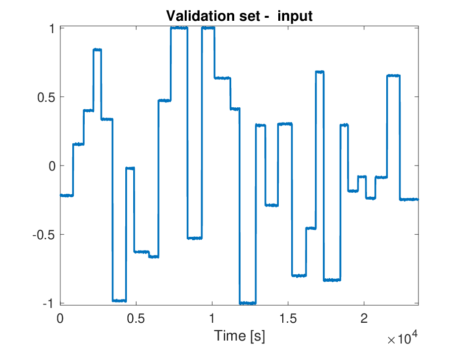

The probabilistic safety verification proposed in Section 3 has then been tested on the LSTM network. In particular, the input class selected for this test is the set of MPRS, with amplitude and with a total duration of time-steps, i.e. seconds. Since , any sequence sampled from is composed by steps with an amplitude uniformly extracted from , and with a random duration uniformly drawn in the range seconds. In Figure (a) some examples of input sequences thus generated have been depicted, for .
The initial state has been extracted from a uniform distribution over . Notice that, owing to LSTM’s ISS, the effect of the initial state asymptotically vanishes.
In light of condition (11), to have a violation probability with confidence , scenarios must be generated. Problem (10) is hence evaluated for different values of , namely for , both for the LSTM network and the real system. Remarkably, the results reported in Figure (b) witness that the LSTM is guaranteed to operate almost in the same region of the real system, i.e. a ball with radius .
[]
\subfigure[]![[Uncaptioned image]](1912.04377v2/verification.png)
5 Conclusions
In this work, the stability properties of LSTM neural networks have been investigated. In particular, a condition on LSTM’s parameters to guarantee the Input-to-State Stability property of the network has been derived, which can be possibly enforced during the training procedure. A probabilistic method for the safety verification of the trained network has then been formulated, which allows – for any class of input signals – to retrieve a tight bound on network’s output reachable set, up to a desired confidence level. The proposed algorithm has been eventually tested on a well-known benchmark system, the pH neutralization process, showing satisfactory performances.
Appendix A Proof of Theorem 4
Let us define the following variables, for the sake of conciseness:
| (13) | ||||||
By means of these definitions, the state equations (2a) and (2b) can be written as
| (14a) | ||||
| (14b) | ||||
Letting , , and , it is possible to re-write (14) as
| (15) |
In light of Theorem 3, consider the following candidate ISS-Lyapunov function:
| (16) |
By definition . Condition (6a) follows trivially, since for a generic vector it holds that . Therefore, condition (6a) is fulfilled taking
We now compute , showing that there exist functions , and fulfilling condition (6b). Using (15) one obtains
In view of the Lipschitzianity of the activation function , it holds that , thus
Recalling the definition of in (13), it holds that
| (17) | ||||
Let , where is the unitary column vector with length . From (3), it follows that . By means of this, we can provide an upper bound for :
Similarly,
In view of these bounds, conditions (7) ensure the existence of a strictly positive scalar such that
| (18) | ||||
for any . Moreover, in light of (1a), it follows that , and are upper-bounded by . Combining (17) and (18), and since and , it is possible to derive that
In view of these results, it is possible to conclude that conditions (6b) are satisfied with
System (15) admits a time invariant ISS-Lyapunov function and, in view of Theorem 3, it is ISS.
References
- Amrouche et al. (2018) Massinissa Amrouche et al. Long short-term memory neural network equilibria computation and analysis. NIPS 2018 Workshop Spatiotemporal Blind Submission, 2018.
- Azoff (1994) E Michael Azoff. Neural network time series forecasting of financial markets. John Wiley & Sons, Inc., 1994.
- Barabanov and Prokhorov (2002) Nikita E Barabanov and Danil V Prokhorov. Stability analysis of discrete-time recurrent neural networks. IEEE Transactions on Neural Networks, 13(2):292–303, 2002.
- Bayer et al. (2013) Florian Bayer, Mathias Bürger, and Frank Allgöwer. Discrete-time incremental ISS: A framework for robust NMPC. In 2013 European Control Conference (ECC), pages 2068–2073. IEEE, 2013.
- Bravo et al. (2006) José M Bravo, Teodoro Alamo, and Eduardo F Camacho. Robust MPC of constrained discrete-time nonlinear systems based on approximated reachable sets. Automatica, 42(10):1745–1751, 2006.
- Bugliari Armenio et al. (2019) Luca Bugliari Armenio, Enrico Terzi, Marcello Farina, and Riccardo Scattolini. Model predictive control design for dynamical systems learned by echo state networks. IEEE Control Systems Letters, 3(4):1044–1049, 2019.
- Bugliari Armenio et al. (2020) Luca Bugliari Armenio, Lorenzo Fagiano, Enrico Terzi, Marcello Farina, and Riccardo Scattolini. Scenario optimization for optimal training of echo state networks. IFAC World Congress 2020 (accepted), 2020.
- Campi et al. (2009) Marco C Campi, Simone Garatti, and Maria Prandini. The scenario approach for systems and control design. Annual Reviews in Control, 33(2):149–157, 2009.
- Deka et al. (2019) Shankar A Deka, Dušan M Stipanović, Boris Murmann, and Claire J Tomlin. Global asymptotic stability and stabilization of long short-term memory neural networks with constant weights and biases. Journal of Optimization Theory and Applications, 181(1):231–243, 2019.
- Fazlyab et al. (2019a) Mahyar Fazlyab, Manfred Morari, and George J Pappas. Probabilistic verification and reachability analysis of neural networks via semidefinite programming. arXiv preprint arXiv:1910.04249, 2019a.
- Fazlyab et al. (2019b) Mahyar Fazlyab, Manfred Morari, and George J Pappas. Safety verification and robustness analysis of neural networks via quadratic constraints and semidefinite programming. arXiv preprint arXiv:1903.01287, 2019b.
- Filippetti et al. (1995) Fiorenzo Filippetti, Giovanni Franceschini, and Carla Tassoni. Neural networks aided on-line diagnostics of induction motor rotor faults. Conference Record of the 1993 IEEE Industry Applications Conference Twenty-Eighth IAS Annual Meeting, 1995.
- Gers and Schmidhuber (2001) Felix A Gers and E Schmidhuber. LSTM recurrent networks learn simple context-free and context-sensitive languages. IEEE Transactions on Neural Networks, 12(6):1333–1340, 2001.
- Greff et al. (2016) Klaus Greff, Rupesh K Srivastava, Jan Koutník, Bas R Steunebrink, and Jürgen Schmidhuber. LSTM: A search space odyssey. IEEE Transactions on Neural Networks and Learning Systems, 28(10):2222–2232, 2016.
- Hall and Seborg (1989) Raymond C Hall and Dale E Seborg. Modelling and self-tuning control of a multivariable pH neutralization process part I: Modelling and multiloop control. In 1989 American Control Conference, pages 1822–1827. IEEE, 1989.
- Haykin (1994) Simon Haykin. Neural networks: a comprehensive foundation. Prentice Hall PTR, 1994.
- Hewing and Zeilinger (2019) Lukas Hewing and Melanie N Zeilinger. Scenario-based probabilistic reachable sets for recursively feasible stochastic model predictive control. IEEE Control Systems Letters, 4(2):450–455, 2019.
- Hochreiter (1998) Sepp Hochreiter. The vanishing gradient problem during learning recurrent neural nets and problem solutions. International Journal of Uncertainty, Fuzziness and Knowledge-Based Systems, 6(02):107–116, 1998.
- Hochreiter and Schmidhuber (1997) Sepp Hochreiter and Jürgen Schmidhuber. Long short-term memory. Neural computation, 9(8):1735–1780, 1997.
- Jaeger (2002) Herbert Jaeger. Tutorial on training recurrent neural networks, covering BPPT, RTRL, EKF and the” echo state network” approach, volume 5. GMD-Forschungszentrum Informationstechnik Bonn, 2002.
- Jiang and Wang (2001) Zhong-Ping Jiang and Yuan Wang. Input-to-state stability for discrete-time nonlinear systems. Automatica, 37(6):857–869, 2001.
- Lanzetti et al. (2019) Nicolas Lanzetti, Ying Z Lian, Andrea Cortinovis, Luis Dominguez, Mehmet Mercangöz, and Colin Jones. Recurrent neural network based MPC for process industries. In 2019 18th European Control Conference (ECC), pages 1005–1010. IEEE, 2019.
- Maler (2008) Oded Maler. Computing reachable sets: An introduction. Tech. rep. French National Center of Scientific Research, 2008.
- Mandic and Chambers (2001) Danilo P Mandic and Jonathon Chambers. Recurrent neural networks for prediction: learning algorithms, architectures and stability. John Wiley & Sons, Inc., 2001.
- Miller and Hardt (2018) John Miller and Moritz Hardt. Stable recurrent models. arXiv preprint arXiv:1805.10369, 2018.
- Pascanu et al. (2013) Razvan Pascanu, Tomas Mikolov, and Yoshua Bengio. On the difficulty of training recurrent neural networks. In International conference on machine learning, pages 1310–1318, 2013.
- Sohrab (2003) Houshang H Sohrab. Basic real analysis, volume 231. Springer, 2003.
- Sontag (1995) Eduardo D Sontag. On the input-to-state stability property. European Journal of Control, 1(1):24–36, 1995.
- Stipanović et al. (2018) Dušan M Stipanović et al. Some local stability properties of an autonomous long short-term memory neural network model. In 2018 IEEE International Symposium on Circuits and Systems (ISCAS), pages 1–5. IEEE, 2018.