Learning a Neural 3D Texture Space from 2D Exemplars
Abstract
We propose a generative model of 2D and 3D natural textures with diversity, visual fidelity and at high computational efficiency. This is enabled by a family of methods that extend ideas from classic stochastic procedural texturing (Perlin noise) to learned, deep, non-linearities. The key idea is a hard-coded, tunable and differentiable step that feeds multiple transformed random 2D or 3D fields into an MLP that can be sampled over infinite domains. Our model encodes all exemplars from a diverse set of textures without a need to be re-trained for each exemplar. Applications include texture interpolation, and learning 3D textures from 2D exemplars. Project website: https://geometry.cs.ucl.ac.uk/projects/2020/neuraltexture.
1 Introduction
Textures are stochastic variations of attributes over 2D or 3D space with applications in both image understanding and synthesis. This paper suggests a generative model of natural textures. Previous texture models either capture a single exemplar (e. g., wood) alone or address non-stochastic (stationary) variation of appearance across space: Which location on a chair should have a wood color? Which should be cloth? Which metal? Our work combines these two complementary views.

Requirements
We design the family of methods with several requirements in mind: completeness, generativeness, compactness, interpolation, infinite domains, diversity, infinite zoom, and high speed.
A space of textures is complete, if every natural texture has a compact code in that embedding. To be generative, every texture code should map to a useful texture. This is important for intuitive design where a user manipulates the texture code and expects the outcome to be a texture. Compactness is achieved if codes are low-dimensional. We also demand the method to provide interpolation: texture generated at coordinates between and should also be valid. This is important for design or when storing texture codes into a (low-resolution) 2D image, 3D volume or at mesh vertices with the desire to interpolate. The first four points are typical for generative modelling; achieving them jointly while meeting more texture-specific requirements (stochasticity, efficiency) is our key contribution.
First, we want to support infinite domains: Holding the texture code fixed, we want to be able to query this texture so that a patch around any position has the statistics of the exemplar. This is important for querying textures in graphics applications for extended virtual worlds, i. e., grass on a football field where it extends the size of the texture.
Second, for visual fidelity, the statistics under which textures are similar to the exemplar. The Gram matrix of VGG activations is one established metric for this similarity [5].
Third, infinite zoom means each texture should have variations on a wide range of scales and not be limited to any fixed resolution that can be held in memory. This is required to zoom into details of geometry and appreciate the fine variation such as wood grains, etc. In practice, we are limited by the frequency content of the exemplars we train on, but the method should not impose any limitations across scales.
Fourth and finally, our aim is computational efficiency: the texture needs to be queryable without requiring prohibitive amounts of memory or time, in any dimension. Ideally, it would be constant in both and parallel. This rules out simple convolutional neural networks, that do not scale favorable in memory consumption to 3D.
2 Previous Work
Capturing the variations of nature using stochastic on many scales has a long history [14]. Making noise useful for graphics and vision is due to Perlin’s 1995 work [17]. Here, textures are generated by computing noise at different frequencies and mixing it with linear weights. A key benefit is that this noise can be evaluated in 2D as well as in 3D making it popular for many graphics applications.
Computer vision typically had looked into generating textures from exemplars, such as by non-parametric sampling [4], vector quantization [25], optimization [12] or nearest-neighbor field synthesis (PatchMatch [2]) with applications in in-painting and also (3D) graphics. Typically, achieving spatial and temporal coherence as well as scalability to fine spatial details remains a challenge. Such classic methods cater to the requirements of human texture perception as stated by Julesz [9]: a texture is an image full of features that in some representation have the same statistics.
The next level of quality was achieved when representations became learned, such as the internal activations of the VGG network [22]. Neural style transfer [5] looked into the statistics of those features, in particular, their Gram matrices. By optimizing over pixel values, these approaches could produce images with the desired texture properties. If these properties are conditioned on existing image structures, the process is referred to as style transfer. VGG was also used for optimization-based multi-scale texture synthesis [20]. Such methods require optimizations for each individual exemplar.
Ulyanov et al. [23] and Johnson et al. [8] have proposed networks that directly produce the texture without optimization. While now a network generated the texture, it was still limited to one exemplar, and no diversity was demonstrated. However, noise at different resolutions [17] is input to these methods, also an inspiration to our work. Follow up work [24] has addressed exactly this difficulty by introducing an explicit diversity term i. e., asking all results in a batch to be different. Unfortunately, this frequently introduces mid-frequency oscillations of brightness that appear admissible to VGG instead of producing true diversity. In our work, we achieve diversity, by restricting the networks input to stochastic values only, i. e., diversity-by-construction
A certain confusion can be noted around the term “texture”. In the human vision [9] and computer vision literature [4, 6], it exclusively refers to stochastic variation. In computer graphics, e. g., OpenGL, “texture” can model both stochastic and non-stochastic variation of color. For example, Visual Object Networks [29] generate a voxel representation of shape and diffuse albedo and refer to the localized color appearance, e. g., wheels of a car are dark, the rim are silver, etc., as “texture”. Similar, Oechsle et al. [16] and Saito et al. [19] use an implicit function to model this variation of appearance in details beyond voxel resolution. Our comparison will show, how methods tackling space of non-stochastic texture variation [16, 29], unfortunately are not suitable to model stochastic appearance. Our work is progress towards learning spaces of stochastic and non-stochastic textures.
Some work has used adversarial training to capture the essence of textures [21, 3], including the non-stationary case [28] or even inside a single image [21]. In particular StyleGAN [10] generates images with details by transforming noise in adversarial training. We avoid the challenges of adversarial training but train a NN to match VGG statistics.
Aittala et al. [1] have extended Gatsy et al.’s 2015 [5] approach to not only generate color, but also ensembles of 2D BRDF model parameter maps from single 2D exemplars. Our approach is compatible with this approach, for example to generate 3D bump, specular, etc. maps, but from 2D input.
At any rate, none of the texture works in graphics or vision [17, 5, 23, 4, 2, 26, 27] generate a space of textures, such as we suggest here, but all work on a single texture while the ones that work on a space of exemplars [29, 16] do not create stochastic textures. Our work closes this gap, by creating a space of stochastic textures.
The graphics community, however, has looked into generating spaces of textures [15], which we here revisit from a deep learning perspective. Their method deforms all pairs of exemplars to each other and constructs a graph with edges that are valid for interpolation when there is evidence that the warping succeeded. To blend between them, histogram adjustments are made. Consequently, interpolation between exemplars is not a straight path from one another, but a traversal along valid observations. Similarly, our method could also construct valid paths in the latent space interpolation.
Finally, all these methods require to learn the texture in the same space it will be used, while our approach can operate in any dimension and across dimensions, including the important case of generating procedural 3D solid textures from 2D observations [11] or slices [18] only.
Summary
| Method |
Diverse |
Details |
Speed |
3D |
Quality |
Space |
2D-to-3D | ||
|---|---|---|---|---|---|---|---|---|---|
| • | Perlin | perlin | ✓ | ✓ | ✓ | ✓ |
✕ |
✕ |
✕ |
| • | Perlin + transform | perlinT | ✓ | ✓ | ✓ | ✓ |
✕ |
✕ |
✕ |
| • | CNN | cnn |
✕ |
✕ |
✕ |
✕ |
✓ |
✕ |
✕ |
| • | CNN + diversity | cnnD | ✓ |
✕ |
✕ |
✕ |
✕ |
✕ |
✕ |
| • | MLP | mlp |
✕ |
✕ |
✓ | ✓ |
✕ |
✕ |
✓ |
| • | Ours + position | oursP |
✕ |
✓ | ✓ | ✓ |
✕ |
✓ | ✓ |
| • | Ours - transform | oursNoT |
✕ |
✕ |
✓ | ✓ | ✓ | ✓ | ✓ |
| • | Ours | ours | ✓ | ✓ | ✓ | ✓ | ✓ | ✓ | ✓ |
The state of the art is depicted in Tbl. 1. Rows list different methods while columns address different aspects of each method. A method is “Diverse” if more than a single exemplar can be produced. MLP [16] is not diverse as the absolute position allows overfitting. We denote a method to have “Detail” if it can produce features on all scales. CNN does not have details, as, in particular in 3D, it needs to represent the entire domain in memory, while MLPs and ours are point operations. “Speed” refers to computational efficiency. Due to high bandwidth and lacking data parallelism, a CNN, in particular in 3D, is less efficient than ours. This prevents application to “3D”. “Quality” refers to visual fidelity, a subjective property. CNN, MLP and ours achieve this, but Perlin is too simple a model. CNN with diversity [24] have decent quality, but a step back from [23]. Our approach creates a “Space” of a class of textures, while all others only work with single exemplars. Finally, our approach allows to learn from a single 2D observation i. e., 2D-to-3D. MLP [16] also learn from 2D images, but have multiple images of one exemplar, and pixels are labeled with depth.
3 Overview
Our approach has two steps. The first embeds the exemplar into a latent space using an encoder. The second provides sampling at any position by reading noise fields at that position and combining them using a learned mapping to match the exemplar statistics. We now detail both steps.

Encoder
The encoder maps a 2D texture exemplar image to a latent texture code . We use a convolutional neural network to encode the high number of exemplar pixels into a compact latent texture code .
Sampler
Sampling of a texture with code at individual 2D or 3D positions has two steps: a translator and a decoder, which are both described next.
Decoder
Our key idea is to prevent the decoder to access the position and to use a vector of noise values instead. Each is read at different linear transformations of that position from random fields with different seeds . The random field is implemented as an infinite, single-channel 2D or 3D function that has the same random value for all continuous coordinates in each integer lattice cell for one seed . The factors of initialize the decoder to behave similar to Perlins’s octaves for identity . Applying to is similar to Spatial Transformer Networks [7]. (Fig. 3).

These noise values are combined with the extended texture code in a learned way. It is the task of the translator, explained next, to control, given the exemplar, how noise is transformed and to generate an extended texture code.
Translator
The translator maps the texture code to a tuple of parameters required by the decoder: the vector of transformation matrices and an extended texture code vector . The matrices are used to transform the coordinates before reading the noise as explained before. The extended texture parameter code is less compact than the texture code , but allows the sampler to execute more effectively, i. e., do not repeat computations required for different as they are redundant for the same .
See Fig. 4 where for example two transformation matrices with 8 DOF are parameterized by three parameters.
Training
For training, the encoder is fed with a random patch of a random exemplar , followed by the sampler evaluating a regular grid of points in random 2D slices of the target domain to produce a “slice” image (Fig. 5). The seed is held constant per train step, as one lattice cell will map to multiple pixels, and the decoder relies on these being consistent. During inference changing the seed and keeping the texture code will yield diverse textures.
The loss is the distance of Gram matrix of VGG feature activations [5, 8, 24, 23, 1] of the patches and .
If the source and target domain are the same (synthesizing 2D textures from 2D exemplars) the slicing operation is the identity. However, it also allows for the important condition in which the target domain has more dimensions than the source domain, such as learning 3D from 2D exemplars.
Spaces-of
Our method can be used to either fit a single exemplar or an entire space of textures. In the single mode, we directly optimize for the trainable parameters of the decoder. When learning the entire space of textures, the full cascade of encoder , translator and sampler parameters are trained, i. e., jointly.
4 Learning stochastic space coloring
Here we will introduce different implementations of samplers which “color” 2D or 3D space at position . We discuss pros and cons with respect to the requirements from the introduction, ultimately leading to our approach.
Perlin
noise is a simple and effective method to generate natural textures in 2D or 3D [17], defined as
| (1) | ||||
where are the RGB weights for different noise functions which return bilinearly-sampled RGB values from an integer grid. is channel-wise multiplication. Here, is a list of all linear per-layer RGB weights e. g., an 83 vector for the octaves we use. This is a simple latent code, but we will see increasingly complex ones later. Also our encoder is designed such that it can cater to all decoders, even Perlin noise i. e., we can also create a space of textures with a Perlin noise back-end.
Coordinates are multiplied by factors of two (octaves), so with increasing , increasingly smooth noises are combined. This is motivated well in the spectra of natural signals [14, 17], but also limiting. Perlin’s linear scaling allows the noise to have different colors, yet no linear operation can reshape a distribution to match a target. Our work seeks to overcome these two limitations, but tries to retain the desirable properties of Perlin noise: simplicity and computational efficiency as well as generalization to 3D.
Transformed Perlin
relaxes the scaling by powers of two
| (2) | ||||
by allowing each noise to be independently scaled by its own transformation matrix since . Please note, that the choice of noise frequency is now achieved by scaling the coordinates reading the noise. This allows to make use of anisotropic scaling for elongated structures, different orientations or multiple random inputs at the same scale.
CNN
utilizes the same encoder as our approach to generate a texture code that is fed in combination with noise to a convolutional decoder similar to [24].
| (3) | ||||
The CNN is conditioned on without additional translation. Their visual quality is stunning, CNNs are powerful and the loss is able to capture perceptually important texture features, hence CNNs are a target to chase for us in 2D in terms of quality. However, there are two main limitations of this approach we seek to lift: efficiency and diversity.
CNNs do not scale well to 3D in high resolutions. To compute intermediate features at , they need to have access to neighbors. While this is effective and output-sensitive in 2D, it is not in 3D: we need results for 2D surfaces embedded in 3D, and do so in spatial high resolution (say 10241024), but this requires CNNs to compute a full 3D volume with the same order of pixels. While in 2D partial outputs can be achieved with sliding windows, it is less clear how to slide a window in 3D, such that it covers all points required to cover all 3D points that are part of the visible surface.
The second issue is diversity: CNNs are great for producing a re-synthesis of the input exemplar, but it has not been demonstrated that changing the seed will lead to variation in the output in most classic works [23, 8] and in classic style transfer [5] diversity is eventually introduced due to the randomness in SGD. Recent work by Ulyanov and colleagues [24] explicitly incentivizes diversity in the loss. The main idea is to increase the pixel variance inside all exemplars produced in one batch. Regrettably, this often is achieved by merely shifting the same one exemplar slightly spatially or introducing random brightness fluctuations.
MLP
maps a 3D coordinate to appearance:
| (4) | ||||
where . Texture-fields [16] have used this approach to produce what they call “texture”, detailed and high-quality appearance decoration of 3D surfaces, but what was probably not intended is to produce diversity or any stochastic results. At least, there is no parameter that introduces any randomness, so all results are identical. We took inspiration in their work, as it makes use of 3D point operations, that do not require accessing any neighbors and no intermediate storage for features in any dimensions, including 3D. It hence reduces bandwidth compared to CNN, is perfectly data-parallel and scalable. The only aspect missing to make it our colorization operator, required to create a space and evolve from 2D exemplars to 3D textures, is stochasticity.
Ours
combines the noise from transformed Perlin for stochasticity, the losses used in style and texture synthesis CNNs for quality as well as the point operations in MLPs for efficiency as follows:
| (5) |
Different from MLPs that take the coordinate as input, position itself is hidden. Instead of position, we take multiple copies of spatially smooth noise as input, with explicit control of how the noise is aligned in space expressed by the transformations . Hence, the MLP requires to map the entire distribution of noise values such that it suits the loss, resulting in build-in diversity. We chose number of octaves to be 8, i. e., the transformation matrices require values in 2D. The texture code size is 64 and the compact code is 8. The decoder consists of four stacked linear layers, with 128 units each followed by ReLUs. The last layer is 3-valued RGB.
Non-stochastic ablation
seeks to investigate what happens if we do not limit our approach to random variables, but also provide access to deterministic information :
| (6) |
is the same as MLP, but with access to noise. We will see that this effectively removes diversity.
Non-transformed ablation
evaluates, if our method were to read only from multi-scale noise without control over how it is transformed. Its definition
| (7) |

5 Evaluation
Our evaluation covers qualitative (Sec. 5.2) and quantitative (Sec. 5.3) aspects as well as a user study (Sec. 5.4).
5.1 Protocol
We suggest a data set that for which we explore the relation of different methods, according to different metrics to quantify texture similarity and diversity.
Data set
Our data set contains four classes (Wood, Marble, Grass and Rust) of 2D textures, acquired from internet image sources. Each class contains 100 images.
Methods
We compare eight different methods that are competitors, ablations and ours.
As five competitors we study variants of Perlin noise, CNNs and MLPs. perlin implements Perlin noise (Eq. 1, [17]) and perlinT our variant extending it by a linear transformation (Eq. 2). Next, cnn is a classic TextureNet [23] and cnnD the extension to incentivise diversity ([24], Eq. 3). mlp uses an MLP following Eq. 4.
Metrics
We evaluate methods in respect to three metrics: similarity and diversity and a joint measure, success.
Similarity is high, if the result produced has the same statistics as the exemplar in terms of L2 differences of VGG Gram matrices. This is identical to the loss used. Similarity is measured on a single exemplar.
Diversity is not part of the loss, but can be measured on a set of exemplars produced by a method. We measure diversity by looking at the VGG differences between all pairs of results in a set produced for a different random seed. Note, that this does not utilize any reference. Diversity is maximized by generating random VGG responses, yet without similarity.
Success of the entire method is measured as the product of diversity and the maximum style error minus the style error. We apply this metric, as it combines similarity and diversity that are conflicting goals we jointly want to maximize.
Memory and speed are measured at a resolution of 128 pixels/voxels on an Nvidia Titan Xp.
5.2 Quantitative results
| Method | Time | Memory | ||
| 2D | 3D | 2D | 3D | |
| perlin • | 0.18 ms | 0.18 ms | 65 k | 16 M |
| perlinT • | 0.25 ms | 0.25 ms | 65 k | 16 M |
| cnn • | 1.45 ms | 551.59 ms | 8,000 k | 646 M |
| cnnD • | 1.45 ms | 551.59 ms | 8,000 k | 646 M |
| mlp • | 1.43 ms | 1.43 ms | 65 k | 16 M |
| oursP • | 1.44 ms | 1.44 ms | 65 k | 16 M |
| oursNoT • | 1.24 ms | 1.24 ms | 65 k | 16 M |
| ours • | 1.55 ms | 1.50 ms | 65 k | 16 M |
Efficiency
We first look at computational efficiency in Tbl. 2. We see that our method shares the speed and memory efficiency with Perlin noise and MLPs / Texture Fields [16]. Using a CNN [23, 24] to generate 3D textures as volumes is not practical in terms of memory, even at a modest resolution. Ours scales linear with pixel resolution as an MLP is a point-estimate in any dimension that does not require any memory other than its output. A CNN has to store the internal activations of all layers in memory for information exchange between neighbors.
| Method | All | Wood | Grass | Marble | ||||||||
| Sim | Div | Suc | Sim | Div | Suc | Sim | Div | Suc | Sim | Div | Suc | |
| perlin • | 20.6 | 48.0 | 7.0 | 23.8 | 37.9 | 4.9 | 24.6 | 72.8 | 18.1 | 13.3 | 31.8 | 7.84 |
| perlinT • | 19.6 | 48.2 | 7.2 | 18.4 | 39.6 | 5.02 | 25.9 | 65.6 | 13.8 | 14.2 | 38.4 | 8.03 |
| cnn • | 5.4 | 0.5 | 7.5 | 13.4 | 0.5 | 0.07 | 1.9 | 0.5 | 0.14 | 1.1 | 0.3 | 0.08 |
| cnnD • | 3.9 | 48.2 | 7.75 | 3.9 | 35.2 | 5.19 | 4.8 | 59.2 | 20.9 | 3.6 | 48.8 | 8.5 |
| mlp • | 14.1 | 0.0 | 7.98 | 15.7 | 0.0 | 0.0 | 16.7 | 0.0 | 0.0 | 9.6 | 0.0 | 0.0 |
| oursP • | 5.4 | 93.4 | 8.23 | 9.7 | 67.4 | 5.33 | 4.8 | 126 | 21.5 | 1.8 | 84.5 | 9.0 |
| oursNoT • | 8.4 | 94.5 | 8.54 | 18.3 | 74.7 | 5.40 | 5.1 | 120 | 21.7 | 1.9 | 87.0 | 9.3 |
| ours • | 12.1 | 99.7 | 8.82 | 13.3 | 72.5 | 5.48 | 13.6 | 127 | 22.1 | 9.4 | 98.2 | 9.6 |

Fidelity
Fig. 6 and Tbl. 3 summarize similarity, diversity and success of all methods in numbers. ours method (black) comes best in diversity and success on average across all sets (first column in Tbl. 3 and top first plot in Fig. 6). cnn (yellow) and cnnd (green) have better similarity than any of our methods. However, no other method combines similarity with diversity as well as ours. This is visible from the overall leading performance in the final measure, success. This is a substantial achievement, as maximizing for only one goal is trivial: an identity method has zero similarity error while a random method has infinite diversity.
When looking at the similarity, we see that both a cnn and its diverse variant cnnD can perform similar. Perlin noise produces the largest error. In particular, perlinT has a large error, indicating it is not sufficient to merely add a transform. Similar, mlp alone cannot solve the task, as it has no access to noise and need to fit exactly, which is doable for single exemplars, but impossible for a space. oursNoT has error similar to ours, but less diversity.
When looking at diversity, it is clear that both cnn and mlp have no diversity as they either do not have the right loss to incentivize it or have no input to generate it. perlin and perlinT both create some level of diversity, which is not surprising as they are simple remappings of random numbers. However, they do not manage to span the full VGG space, which only ours and its ablations can do.
Generating 3D textures from the exemplar in Fig. 7, we find that our diversity and similarity are 44.5 and 1.48, which compares favorable to Perlin 3D Noise at 14.9 and 7.11.
5.3 Qualitative results
Visual examples from the quantitative evaluation on a single exemplar for different methods can be seen in Fig. 7. We see that some methods have diversity when the seed is changed (rows one vs. two and three vs. four) and some do not. Diversity is clear for Perlin and its variant, CNNs with a diversity term and our approach. No diversity is found for MLPs and CNNs. We also note, that CNNs with diversity produce typically shifted copies of the same exemplar, so their diversity is over-estimated by the metric.

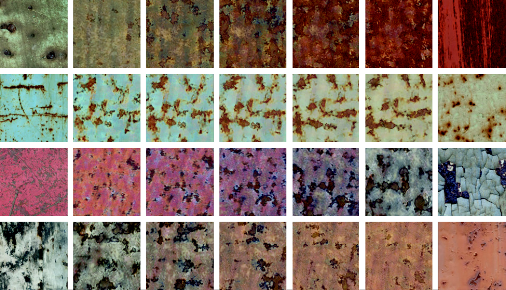
A meaningful latent texture code space should also allow for interpolation as seen in Fig. 8, where we took pairs of texture codes (left and right-most exemplar) and interpolated rows in-between. We see, that different paths produce plausible blends, with details appearing and disappearing, which is not the case for a linear blend (last row).

Our method does not work on an explicit pixel grid, which allows to zoom into arbitrary fine details as show in Fig. 9, comparing favorable to cubic upsampling. This is particularly useful in 3D, where storing a complete volume to span multiple levels of detail requires prohibitive amounts of memory while ours is output-sensitive.

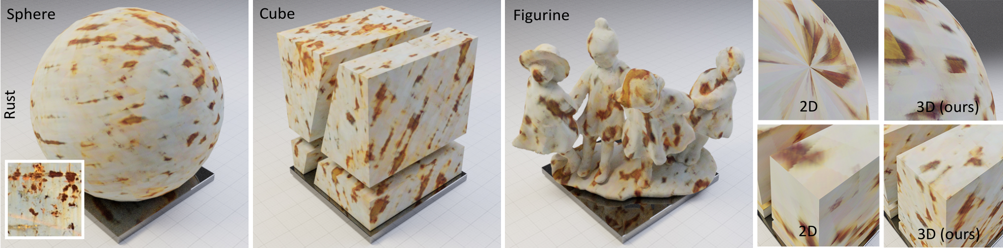

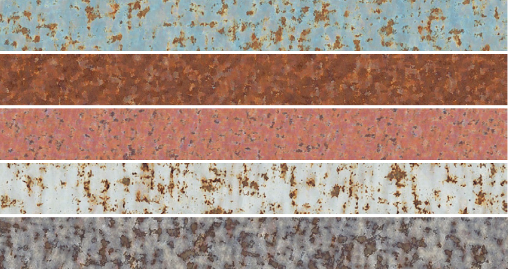
Fig. 10 shows a stripe re-synthesized from a single exemplar. We note that the pattern captures the statistics, but does not repeat.
Fig. 12 documents the ability to reproduce the entire space. We mapped exemplars unobserved at training time to texture codes, from which we reconstruct them, in 2D. We find that our approach reproduces the exemplars faithfully, albeit totally different on the pixel level.
Our system can construct textures and spaces of textures in 3D from 2D exemplars alone. This is shown in Fig. 11. We first notice, that the textures have been transferred to 3D faithfully, inheriting all the benefits of procedural textures in image synthesis. We can now take any shape, without a texture parametrization and by simply running the NN at each pixel’s 3D coordinate produce a color. We compare to a 2D approach by loading the objects in Blender and applying its state-of-the-art UV mapping approach [13]. Inevitably, a sphere will have discontinuities and poles that can not be resolved in 2D, that are no issue to our 3D approach while both take the same 2D as input.
5.4 User study
Presenting pairs of images produced by either perlinT, cnnD, mlp, oursP, oursNoT and ours for one exemplar texture to subjects and asking which result “they prefer” in a two-alternative forced choice, we find that 16.7% prefer the ground truth, 4.9% perlin, 7.7% perlinT, 14.3% cnn, 8.8% cnnD, 9.4% mlp, 10.8% oursNoT, 12.9% oursP and 14.5% ours (statistical significance; , binomial test). Given ground truth and cnn are not diverse, out of all methods that synthesize infinite textures our results are preferred over all other.
6 Conclusion
We have proposed a generative model of natural 3D textures. It is trained on 2D exemplars only, and provides interpolation, synthesis and reconstruction in 3D. The key inspiration is Perlin Noise – now more than 30 years old – revisited with NNs to match complex color relations in 3D according to the statistics of VGG activations in 2D. The approach has the best combination of similarity and diversity compared to a range of published alternatives, that are less computationally efficient.
Reshaping noise to match VGG activations using MLPs can be a scalable solution to other problems in even higher dimensions, such as time, that are difficult for CNNs.
Acknowledgements
This work was supported by the ERC Starting Grant SmartGeometry, a GPU donation by NVIDIA Corporation and a Google AR/VR Research Award.
References
- [1] Miika Aittala, Timo Aila, and Jaakko Lehtinen. Reflectance modeling by neural texture synthesis. ACM Trans. Graph. (Proc. SIGGRAPH), 35(4):65, 2016.
- [2] Connelly Barnes, Eli Shechtman, Adam Finkelstein, and Dan B Goldman. Patchmatch: A randomized correspondence algorithm for structural image editing. ACM Trans. Graph. (Proc. SIGGRAPH), 28(3):24, 2009.
- [3] Urs Bergmann, Nikolay Jetchev, and Roland Vollgraf. Learning texture manifolds with the periodic spatial gan. In J MLR, pages 469–477, 2017.
- [4] Alexei A Efros and Thomas K Leung. Texture synthesis by non-parametric sampling. In ICCV, 1999.
- [5] Leon Gatys, Alexander S Ecker, and Matthias Bethge. Texture synthesis using convolutional neural networks. In NIPS, 2015.
- [6] Aaron Hertzmann, Charles E Jacobs, Nuria Oliver, Brian Curless, and David H Salesin. Image analogies. In Proc. SIGGRAPH, 2001.
- [7] Max Jaderberg, Karen Simonyan, Andrew Zisserman, et al. Spatial transformer networks. In NIPS, pages 2017–2025, 2015.
- [8] Justin Johnson, Alexandre Alahi, and Li Fei-Fei. Perceptual losses for real-time style transfer and super-resolution. In ECCV, 2016.
- [9] Bela Julesz. Texture and visual perception. Scientific American, 212(2), 1965.
- [10] Tero Karras, Samuli Laine, and Timo Aila. A style-based generator architecture for generative adversarial networks. In CVPR, pages 4401–4410, 2019.
- [11] Johannes Kopf, Chi-Wing Fu, Daniel Cohen-Or, Oliver Deussen, Dani Lischinski, and Tien-Tsin Wong. Solid texture synthesis from 2D exemplars. ACM Trans. Graph. (Proc. SIGGRAPH), 26(3):2, 2007.
- [12] Vivek Kwatra, Irfan Essa, Aaron Bobick, and Nipun Kwatra. Texture optimization for example-based synthesis. In ACM Trans. Graph., volume 24, 2005.
- [13] Bruno Lévy, Sylvain Petitjean, Nicolas Ray, and Jérome Maillot. Least squares conformal maps for automatic texture atlas generation. 21(3):362–71, 2002.
- [14] Benoit B Mandelbrot. The fractal geometry of nature, volume 173. WH Freeman New York, 1983.
- [15] Wojciech Matusik, Matthias Zwicker, and Frédo Durand. Texture design using a simplicial complex of morphable textures. ACM Trans. Graph. (Proc. SIGGRAPH), 24(3), 2005.
- [16] Michael Oechsle, Lars Mescheder, Michael Niemeyer, Thilo Strauss, and Andreas Geiger. Texture fields: Learning texture representations in function space. In ICCV, 2019.
- [17] Ken Perlin. An image synthesizer. SIGGRAPH Comput. Graph., 19(3), 1985.
- [18] Nico Pietroni, Miguel A Otaduy, Bernd Bickel, Fabio Ganovelli, and Markus Gross. Texturing internal surfaces from a few cross sections. 26(3), 2007.
- [19] Shunsuke Saito, Zeng Huang, Ryota Natsume, Shigeo Morishima, Angjoo Kanazawa, and Hao Li. PiFu: Pixel-aligned implicit function for high-resolution clothed human digitization. In CVPR, pages 2304–2314, 2019.
- [20] Omry Sendik and Daniel Cohen-Or. Deep correlations for texture synthesis. ACM Trans. Graph., 36(5):161, 2017.
- [21] Tamar Rott Shaham, Tali Dekel, and Tomer Michaeli. SinGAN: Learning a generative model from a single natural image. In ICCV, 2019.
- [22] Karen Simonyan and Andrew Zisserman. Very deep convolutional networks for large-scale image recognition. arXiv:1409.1556, 2014.
- [23] Dmitry Ulyanov, Vadim Lebedev, Andrea Vedaldi, and Victor S Lempitsky. Texture networks: Feed-forward synthesis of textures and stylized images. In ICML, 2016.
- [24] Dmitry Ulyanov, Andrea Vedaldi, and Victor Lempitsky. Improved texture networks: Maximizing quality and diversity in feed-forward stylization and texture synthesis. In CVPR, 2017.
- [25] Li-Yi Wei and Marc Levoy. Fast texture synthesis using tree-structured vector quantization. In Proc. SIGGRAPH, 2000.
- [26] Wenqi Xian, Patsorn Sangkloy, Varun Agrawal, Amit Raj, Jingwan Lu, Chen Fang, Fisher Yu, and James Hays. TextureGAN: Controlling deep image synthesis with texture patches. In CVPR, 2018.
- [27] Ning Yu, Connelly Barnes, Eli Shechtman, Sohrab Amirghodsi, and Michal Lukac. Texture Mixer: A network for controllable synthesis and interpolation of texture. In CVPR, 2019.
- [28] Yang Zhou, Zhen Zhu, Xiang Bai, Dani Lischinski, Daniel Cohen-Or, and Hui Huang. Non-stationary texture synthesis by adversarial expansion. arXiv:1805.04487, 2018.
- [29] Jun-Yan Zhu, Zhoutong Zhang, Chengkai Zhang, Jiajun Wu, Antonio Torralba, Josh Tenenbaum, and Bill Freeman. Visual object networks: Image generation with disentangled 3D representations. In NIPS, 2018.
Appendix A Network Architecture
A.1 Encoder
The architecture for the encoder network remains consistent for both ours and competitor methods. Depending on training for space, single, w/o transform the parameter N changes accordingly.
| Layer | Kernel | Activation | Shape | # params |
|---|---|---|---|---|
| Input | — | — | 3 x 128 x 128 | — |
| Conv | 3x3 | IN+LReLU | 32 x 128 x 128 | 1k |
| Conv | 4x4 | IN+LReLU | 64 x 64 x 64 | 32k |
| Conv | 4x4 | IN+LReLU | 128 x 32 x 32 | 130k |
| Conv | 4x4 | IN+LReLU | 256 x 16 x 16 | 524k |
| Conv | 4x4 | IN+LReLU | 256 x 8 x 8 | 1M |
| Conv | 4x4 | IN+LReLU | 256 x 4 x 4 | 1M |
| Linear | — | — | 8 | 32k |
| Linear | — | — | N | 0.5k |
| # params | — | — | 2.8M |
A.2 Sampler
The sampler architecture used for both our and the mlp [16] method consists of following convolutional architecture with 1x1 kernels emulating Linear layers:
| Layer | Kernel | Activation | Shape | # params |
|---|---|---|---|---|
| Input | — | — | N x 128 x 128 | — |
| Conv | 1x1 | ReLU | 128 x 128 x 128 | 10k |
| Conv | 1x1 | ReLU | 128 x 128 x 128 | 16.5k |
| Conv | 1x1 | ReLU | 128 x 128 x 128 | 16.5k |
| Conv | 1x1 | ReLU | 128 x 128 x 128 | 16.5k |
| Conv | 1x1 | ReLU | 128 x 128 x 128 | 16.5k |
| Conv | 1x1 | ReLU | 3 x 128 x 128 | 400 |
| # params | — | — | 77k |
A.3 CNN
For cnn and cnnD competitors we use a similar architecture to the proposed method of [24]:
| Layer | Kernel | Activation | Shape | # params |
|---|---|---|---|---|
| Input | — | — | (32) + 256 | — |
| Linear | — | — | (32) + 256 | 80k |
| Linear | — | — | 256 | 70k |
| Reshape | — | — | 16 x 4 x 4 | — |
| ConvT | 4x4 | ReLU | 128 x 8 x 8 | 32k |
| ConvT | 4x4 | ReLU | 128 x 16 x 16 | 260k |
| ConvT | 4x4 | ReLU | 128 x 32 x 32 | 260k |
| Upsample | — | — | 128 x 64 x 64 | — |
| Conv | 3x3 | ReLU | 64 x 64 x 64 | 70k |
| Upsample | — | — | 64 x 128 x 128 | — |
| Conv | 3x3 | ReLU | 3 x 128 x 128 | 2k |
| # params | — | — | 790k |
Appendix B Results
Additional results of stripe images and interpolations are displayed below.
A webpage containing more results for all four classes (Wood, Marble, Grass and Rust) including competitors can be accessed online: https://geometry.cs.ucl.ac.uk/projects/2020/neuraltexture. Additionally, videos of rotating shapes textured by our method are provided. Our code is available at: https://github.com/henzler/neuraltexture