跳到论文正文
W Papers独立论文阅读器 arXiv:1912.04135 论文正文 计算阅读时间 · 0%
引用这篇论文根据当前论文元数据生成,正式投稿前建议核对。


License: arXiv.org perpetual non-exclusive license
arXiv:1912.04135v2 [math.CO] 11 Dec 2019

Persistent spectral graph

Rui Wang Affiliation:  Department of Mathematics, Michigan State University, MI 48824, USA    Duc Duy Nguyen Affiliation:  Department of Mathematics, Michigan State University, MI 48824, USA    Guo-Wei Wei Note: Address correspondences to Guo-Wei Wei. E-mail:wei@math.msu.edu Affiliation:  Department of Mathematics, Michigan State University, MI 48824, USA Affiliation:  Department of Biochemistry and Molecular BiologyMichigan State University, MI 48824, USA Affiliation:  Department of Electrical and Computer EngineeringMichigan State University, MI 48824, USA
August 11, 2026
Abstract

Persistent homology is constrained to purely topological persistence while multiscale graphs account only for geometric information. This work introduces persistent spectral theory to create a unified low-dimensional multiscale paradigm for revealing topological persistence and extracting geometric shape from high-dimensional datasets. For a point-cloud dataset, a filtration procedure is used to generate a sequence of chain complexes and associated families of simplicial complexes and chains, from which we construct persistent combinatorial Laplacian matrices. We show that a full set of topological persistence can be completely recovered from the harmonic persistent spectra, i.e., the spectra that have zero eigenvalues, of the persistent combinatorial Laplacian matrices. However, non-harmonic spectra of the Laplacian matrices induced by the filtration offer another power tool for data analysis, modeling, and prediction. In this work, non-harmonic persistent spectra are successfully devised to analyze the structure and stability of fullerenes and predict the B-factors of a protein, which cannot be straightforwardly extracted from the current persistent homology. Extensive numerical experiments indicate the tremendous potential of the proposed persistent spectral analysis in data science.

Key words: Persistent spectral theory, persistent spectral analysis, persistent spectral graph, spectral data analysis.

1 Introduction

Graph theory, a branch of discrete mathematics, concerns the relationship between objects. These objects can be either simple vertices, i.e., nodes and/or points (zero simplexes), or high-dimensional simplexes. Here, the relationship refers to connectivity with possible orientations. Graph theory has many branches, such as geometric graph theory, algebraic graph theory, and topological graph theory. The study of graph theory draws on many other areas of mathematics, including algebraic topology, knot theory, algebra, geometry, group theory, combinatorics, etc. For example, algebraic graph theory can be investigated by using either linear algebra, group theory, or graph invariants. Among them, the use of learning algebra in graph study leads to spectral graph theory.

Precursors of the spectral theory have often had a geometric flavor. An interesting spectral geometry question asked by Mark Kac was “Can one hear the shape of a drum?” [28]. The Laplace-Beltrami operator on a closed Riemannian manifold has been intensively studied [29]. Additionally, eigenvalues and isoperimetric properties of graphs are the foundation of the explicit constructions of expander graphs [26]. Moreover, the study of random walks and rapidly mixing Markov chains utilized the discrete analog of the Cheeger inequality [12]. The interaction between spectral theory and differential geometry became one of the critical developments [18]. For example, the spectral theory of the Laplacian on a compact Riemannian manifold is a central object of de Rham-Hodge theory [29]. Note that the Hodge Laplacian spectrum contains the topological information of the underlying manifold. Specifically, the harmonic part of the Hodge Laplacian spectrum corresponds to topological cycles. Connections between topology and spectral graph theory also play a central role in understanding the connectivity properties of graphs [22, 30, 51, 41]. Similarly, as the topological invariants revealing the connectivity of a topological space, the multiplicity of 00 eigenvalues of a 0-combinatorial Laplacian matrix is the number of connected components of a graph. Indeed, the number of qq-dimensional holes can also be unveiled from the number of 00 eigenvalues of the qq-combinatorial Laplacian [39, 24, 33, 21]. Nonetheless, spectral graph theory offers additional non-harmonic spectral information beyond topological invariants.

The traditional topology and homology are independent of metrics and coordinates and thus, retain little geometric information. This obstacle hinders their practical applicability in data analysis. Recently, persistent homology has been introduced to overcome this difficulty by creating low-dimensional multiscale representations of a given object of interest [19, 17, 52, 15, 34, 11]. Specifically, a filtration parameter is devised to induce a family of geometric shapes for a given initial data. Consequently, the study of the underlying topologies or homology groups of these geometric shapes leads to the so-called topological persistence. Like the de Rham-Hodge theory which bridges differential geometry and algebraic topology, persistent homology bridges multiscale analysis and algebraic topology. Topological persistence is the most important aspect of the popular topological data analysis (TDA) [13, 48, 9, 14] and has had tremendous success in computational biology [46, 10] and worldwide competitions in computer-aided drug design [36].

Graph theory has been applied in various fields [20]. For example, spectral graph theory is applied to the quantum calculation of π\pi-delocalized systems. The Hückel method, or Hückel molecular orbital theory, describes the quantum molecular orbitals of π\pi-electrons in π\pi-delocalized systems in terms of a kind of adjacency matrix that contains atomic connectivity information [5, 23]. Additionally, the Gaussian network model (GNM) [4] and anisotropic network model (ANM) [2] represent protein Cα atoms as an elastic mass-and-spring network by graph Laplacians. These approaches were influenced by the Flory theory of elasticity and the Rouse model [3]. Like traditional topology, traditional graph theory extracts very limited information from data. In our earlier work, we have proposed multiscale graphs, called multiscale flexibility rigidity index (mFRI), to describe the multiscale nature of biomolecular interactions [38], such as hydrogen bonds, electrostatic effects, van der Waals interactions, hydrophilicity, and hydrophobicity. A multiscale spectral graph method has also been proposed as generalized GNM and generalized ANM [44]. Our essential idea is to create a family of graphs with different characteristic length scales for a given dataset. We have demonstrated that our multiscale weighted colored graph (MWCG) significantly outperforms traditional spectral graph methods in protein flexibility analysis [8]. More recently, we demonstrate that our MWCG outperforms other existing approaches in protein-ligand binding scoring, ranking, docking, and screening [35].

The objective of the present work is to introduce persistent spectral graph as a new paradigm for the multiscale analysis of the topological invariants and geometric shapes of high-dimensional datasets. Motivated by the success of persistent homology [10] and multiscale graphs [35] in dealing with complex biomolecular data, we construct a family of spectral graphs induced by a filtration parameter. In the present work, we consider the radius filtration via the Vietoris-Rips complex while other filtration methods can be implemented as well. As the filtration radius is increased, a family of persistent qq-combinatorial Laplacians are constructed for a given point-cloud dataset. The diagonalization of these persistent qq-combinatorial Laplacian matrices gives rise to persistent spectra. It is noted that our harmonic persistent spectra of 0-eigenvalues fully recover the persistent barcode or persistent diagram of persistent homology. Additional information is generated from non-harmonic persistent spectra, namely, the non-zero eigenvalues and associated eigenvectors. In a combination with a simple machine learning algorithm, this additional spectral information is found to provide a powerful new tool for the quantitative analysis of molecular data.

2 Theories and methods

In this section, we give a brief review of spectral graph theory and simplicial complex to establish notations and provide essential background. Subsequently, we introduce persistent spectral analysis.

2.1 Spectral graph theory

Graph structure encodes inter-dependencies among constituents and provides low-dimensional representations of high-dimensional datasets. One of the representations frequently used in spectral graph theory (SGT) is to associate graphs with matrices, such as the Laplacian matrix and adjacency matrix. Analyzing the spectra from such matrices leads to the understanding of the topological and spectral properties of the graph.

Let VV be the vertex set, and EE be the edge set. For a given simple graph G⁡(V,E)G(V,E) (A simple graph can be either connected or disconnected), the degree of the vertex v∈Vv\in V is the number of edges that are adjacent to vv, denoted deg​(v)\text{deg}(v). The adjacency matrix 𝒜\mathcal{A} is defined by

𝒜⁡(G)={1if vi and vj are adjacent,0otherwise.\mathcal{A}(G)=\begin{cases}1&\mbox{if $v_{i}$ and $v_{j}$ are adjacent,}\\ 0&\mbox{otherwise}.\end{cases} (1)

and the Laplacian matrix ℒ\mathcal{L} is given by

ℒ⁡(G)={deg​(vi)if vi=vj,−1if vj and vj are adjacent,0otherwise.\mathcal{L}(G)=\begin{cases}\text{deg}(v_{i})&\mbox{if $v_{i}=v_{j}$,}\\ -1&\mbox{if $v_{j}$ and $v_{j}$ are adjacent,}\\ 0&\mbox{otherwise}.\end{cases} (2)

Obviously, the adjacency matrix characterizes the graph connectivity. The above two matrices are related through diagonal matrix 𝒟\mathcal{D}

ℒ=𝒟−𝒜\mathcal{L}=\mathcal{D}-\mathcal{A}

Assuming G⁡(V,E)G(V,E) has NN nodes, then adjacency matrix 𝒜\mathcal{A} and Laplacian matrix ℒ\mathcal{L} are both real symmetric N×NN\times N matrices. The eigenvalues of adjacency and Laplacian matrices are denoted and ordered as

αmin=αN≤⋯≤α2≤α1=αmaxλmin=λ1≤λ2≤⋯≤λN=λmax.\begin{split}\alpha_{\min}=\alpha_{N}\leq\cdots\leq\alpha_{2}\leq\alpha_{1}=\alpha_{\max}\\ \lambda_{\min}=\lambda_{1}\leq\lambda_{2}\leq\cdots\leq\lambda_{N}=\lambda_{\max}.\end{split} (3)

The spectra of 𝒜\mathcal{A} and ℒ\mathcal{L} have several interesting proprieties as following [51].

Property 2.1.

The eigenvalues of adjacency matrix 𝒜\mathcal{A} lie in the interval [−d,d][-d,d] with dd being the largest vertex degree of graph G⁡(V,E)G(V,E).

Property 2.2.

A graph is bipartite if and only if its adjacency spectrum is symmetric about 0.

Property 2.3.

The Laplacian matrix ℒ\mathcal{L} is positive semi-defined, all eigenvalues of ℒ\mathcal{L} are non-negative and lie in the interval [0,2​d][0,2d] with dd being the largest vertex degree of graph G⁡(V,E)G(V,E).

Except for the aforementioned proprieties for adjacency and Laplacian matrices, one also analyzes the upper and lower bounds for algebraic connectivity λ2\lambda_{2} and the largest Laplacian eigenvalue λN\lambda_{N} of graphs. This analysis helps to understand the robustness and connectivity of a graph. For more detailed theorems and proofs, we refer the interested reader to a survey on Laplacian eigenvalues of graphs [51].

Theorem 2.1.

Let G⁡(V,E)G(V,E) be a simple graph of order NN, then the multiplicity of 00 eigenvalue for Laplacian matrix is the number of connected components of G⁡(V,E)G(V,E). The vertex degree is the value of the diagonal entry.

Theorem 2.2.

Let G⁡(V,E)G(V,E) be a simple graph of order NN, then the largest eigenvalue

λN≤max⁡{deg​(u)+deg​(v)|(u,v)∈E},\lambda_{N}\leq\max\{\text{deg}(u)+\text{deg}(v)|(u,v)\in E\}, (4)

where deg​(u)\text{deg}(u) is the degree of vertex u∈Vu\in V.

Theorem 2.3.

Let G⁡(V,E)G(V,E) be a simple graph of order NN rather than a complete graph with vertex connectivity κ⁡(G)\kappa(G) and edge connectivity κ′​(G)\kappa^{\prime}(G). Then

2​κ′​(G)​(1−cos⁡(π/N))≤λ2​(G)≤κ⁡(G)≤κ′​(G).2\kappa^{\prime}(G)(1-\cos(\pi/N))\leq\lambda_{2}(G)\leq\kappa(G)\leq\kappa^{\prime}(G). (5)

The vertex connectivity κ⁡(G)\kappa(G) is the minimum number of nodes whose deletion disconnects GG and edge connectivity κ′​(G)\kappa^{\prime}(G) to be the minimum number of edges whose deletion from a graph GG disconnects GG.

Remark 2.1.

In this section, the Laplacian spectrum of simple graph G⁡(V,E)G(V,E) is concerned. For

G(V,E)=G1(V1,E1)⋃⋯⋃Gm(Vm,Em),m≥1,m∈ℤ,G(V,E)=G_{1}(V_{1},E_{1})\bigcup\cdots\bigcup G_{m}(V_{m},E_{m}),m\geq 1,m\in\mathbb{Z},

where Gi(Vi,Ei)⊂G(V,E),i=1,⋯,mG_{i}(V_{i},E_{i})\subset G(V,E),i=1,\cdots,m is a connected simple graph. If m≥2m\geq 2, the zero eigenvalue of L⁡(G)L(G) has multiplicity mm, which results in algebraic connectivity λ2=0\lambda_{2}=0. However, λ2=0\lambda_{2}=0 cannot give any information about the Gi​(Vi,Ei)G_{i}(V_{i},E_{i}). Therefore, we study the smallest non-zero eigenvalue of L⁡(G)L(G), which is actually the smallest algebraic connectivity of ℒ⁡(Gi),i=1,⋯,m\mathcal{L}(G_{i}),i=1,\cdots,m. In subsection 2.3 and section 3, we analyze the smallest non-zero eigenvalue of the Laplacian matrix. To make the expression more concise, we still use λ~𝟐\mathbf{\tilde{\lambda}_{2}} as the smallest non-zero eigenvalue. If G⁡(V,E)G(V,E) is a connected simple graph, i.e., m=1m=1, one has λ2=λ~2\lambda_{2}=\tilde{\lambda}_{2}.

The charts in the top row of Figure 1 show 55 different types of regular convex polyhedrons, which are called platonic solids. The charts in the bottom row are platonic graphs that intuitively describe the vertices and edges as points and line segments in the Euclidean plane. In the three-dimensional (3D) space, objects (vertices) and the relationship (edges) between objects can be expressed by the Laplacian matrix and vice versa. Taking tetrahedron as an example, we denote the top vertex as v1v_{1}, while the other 33 vertices on the plane are denoted as v2,v3v_{2},v_{3}, and v4v_{4}. The Laplacian matrix of the tetrahedron can be expressed as:

ℒTetra=[3−1−1−1−13−1−1−1−13−1−1−1−13]\mathcal{L}_{\text{Tetra}}=\left[\begin{array}[]{cccc}3&-1&-1&-1\\ -1&3&-1&-1\\ -1&-1&3&-1\\ -1&-1&-1&3\end{array}\right]

with eigenvalues being λ1=0,λ2=4,λ3=4,\lambda_{1}=0,\lambda_{2}=4,\lambda_{3}=4, and λ4=4\lambda_{4}=4. Topological information can be extracted from this Laplacian matrix. First, the multiplicity of 00 eigenvalue is 11, which means there is only one connected component. Secondly, all of the entries in LTetraL_{\text{Tetra}} are non-zero and all the entries in the diagonal equal to 33, which means the corresponding graph is a complete 33-regular graph. Moreover, as stated by Theorems 2.2 and 2.3, the largest eigenvalue λ4≤max⁡{deg​(u)+deg​(v)|(u,v)∈E}=6\lambda_{4}\leq\max\{\text{deg}(u)+\text{deg}(v)|(u,v)\in E\}=6. The second smallest eigenvalue λ2\lambda_{2} is controlled by κ⁡(G)=4\kappa(G)=4 and greater than 2​κ′​(G)​(1−cos⁡(π/N))=2×3×(1−cos⁡(π/4))≈1.757359312882\kappa^{\prime}(G)(1-\cos(\pi/N))=2\times 3\times(1-\cos(\pi/4))\approx 1.75735931288. A similar analysis can be applied to other 44 platonic solids. Table 1 shows some characteristics of platonic solids.

Refer to caption
Figure 1: Platonic solids (top row) and its platonic graphs (bottom row). (a) Tetrahedron and tetrahedral graph. (b) Octahedron and octahedral graph. (c) Cube and cubical graph. (d) Dodecahedron and dodecahedral graph. (e) Icosahedron and icosahedral graph.
Table 1: Characteristics of platonic solids in Figure 1. V,E,β0,κ,κ′,d,V,E,\beta_{0},\kappa,\kappa^{\prime},d, and λ~2\tilde{\lambda}_{2} stand for the number of vertices, the number of edges, the number of zero eigenvalues, vertex connectivity, edge connectivity, and the smallest non-zero eigenvalue, respectively. Here, all the platonic graphs are connected simple graphs, so λ2=λ~2\lambda_{2}=\tilde{\lambda}_{2}.
  Platonic Solid   VV   EE   κ\kappa   κ′\kappa^{\prime}   β0\beta_{0}   λ~2\tilde{\lambda}_{2}
  Tetrahedron   44   66   44   33   11   4.004.00
  Octahedron   66   1212   44   44   11   4.004.00
  Cube   88   1212   33   33   11   2.002.00
  Dodecahedron   2020   3030   33   33   11   0.76390.7639
  Icosahedron   1212   3030   55   55   11   2.762.76

2.2 Simplicial complex

A simplicial complex is a powerful algebraic topology tool that has wide applications in graph theory, topological data analysis [15], and many physical fields [10]. We briefly review simplicial complexes to generate notation and provide essential preparation for introducing persistent spectral graph.

2.2.1 Simplex

Let {v0,v1,⋯,vq}\{v_{0},v_{1},\cdots,v_{q}\} be a set of points in ℝn\mathbb{R}^{n}. A point v=∑i=0qλi​vi,λi∈ℝv=\displaystyle{\sum_{i=0}^{q}}\lambda_{i}v_{i},\lambda_{i}\in\mathbb{R} is an affine combination of viv_{i} if ∑i=0qλi=1\displaystyle{\sum_{i=0}^{q}}\lambda_{i}=1. An affine hull is the set of affine combinations. Here, q+1q+1 points v0,v1,⋯,vqv_{0},v_{1},\cdots,v_{q} are affinely independent if v1−v0,v2−v0,⋯,vq−v0v_{1}-v_{0},v_{2}-v_{0},\cdots,v_{q}-v_{0} are linearly independent. A qq-plane is well-defined if the q+1q+1 points are affinely independent. In ℝn\mathbb{R}^{n}, one can have at most nn linearly independent vectors. Therefore, there are at most n+1n+1 affinely independent points. An affine combination v=∑i=0qλi​viv=\displaystyle{\sum_{i=0}^{q}}\lambda_{i}v_{i} is a convex combination if all λi\lambda_{i} are non-negative. The convex hull is the set of convex combinations.

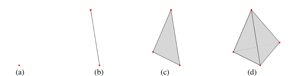
A (geometric) qq-simplex denoted as σq\sigma_{q} is the convex hull of q+1q+1 affinely independent points in ℝn​(n≥q)\mathbb{R}^{n}(n\geq q) with dimension dim​(σq)=q\text{dim}(\sigma_{q})=q. A 00-simplex is a vertex, a 11-simplex is an edge, a 22-simplex is a triangle, and a 33-simplex is a tetrahedron, as shown in Figure 2. The convex hull of each nonempty subset of q+1q+1 points forms a subsimplex and is regraded as a face of σq\sigma_{q} denoted τ\tau. The pp-face of a qq-simplex is the subset {vi​1,⋯,vi​p}\{v_{i1},\cdots,v_{ip}\} of the qq-simplex.

Refer to caption
Figure 2: Illustration of simplices. (a) 00-simplex (a vertex), (b) 11-simplex (an edge), (c)(c) 22-simplex (a triangle), and (d) 33-simplex (a tetrahedron)

2.2.2 Simplicial complex

A (finite) simplicial complex KK is a (finite) collection of simplices in ℝn\mathbb{R}^{n} satisfying the following conditions

  • (1)

    If σq∈K\sigma_{q}\in K and σp\sigma_{p} is a face of σq\sigma_{q}, then σp∈K\sigma_{p}\in K.

  • (2)

    The non-empty intersection of any two simplices σq,σp∈K\sigma_{q},\sigma_{p}\in K is a face of both of σq\sigma_{q} and σp\sigma_{p}.

Each element σq∈K\sigma_{q}\in K is a qq-simplex. The dimension of KK is defined as dim​(K)=max⁡{dim​(σq):σq∈K}\text{dim}(K)=\max\{\text{dim}(\sigma_{q}):\sigma_{q}\in K\}. To distinguish topological spaces based on the connectivity of simplicial complexes, one uses Betti numbers. The kk-th Betti number, βk\beta_{k}, counts the number of kk-dimensional holes on a topological surface. The geometric meaning of Betti numbers in ℝ3\mathbb{R}^{3} is the following: β0\beta_{0} represents the number of connected components, β1\beta_{1} counts the number of one-dimensional loops or circles, and β2\beta_{2} describes the number of two-dimensional voids or holes. In a nutshell, the Betti number sequence {β0,β1,β2,⋯}\{\beta_{0},\beta_{1},\beta_{2},\cdots\} reveals the intrinsic topological property of the system. To illustrate the simplicial complex and its corresponding Betti number, we have designed two simple models as is shown in Figure 3. 11 1 These examples show in an intuitive way to count Betti numbers. However, In subsection 2.3, it is impossible to generate structures (b), (e), and (f).

Refer to caption
Figure 3: Illustrations of simplicial complexes
Table 2: The Betti number of simplicial complexes in Figure 3. Each color represents different faces. The tetrahedron-shaped simplicial complexes are demonstrated in (a)-(c), and the cube-shaped simplicial complexes are depicted in (d) - (f). (a) and (d) only has 00-simplices and 11-simplices, (b) has four 22-simplices, and (c) has one more 33-simplex. (e) and (f) do not have any 22-simplex.
Betti number Fig. 33 (a) Fig. 33 (b) Fig. 33 (c) Fig. 33 (d) Fig. 33 (e) Fig. 33 (f)
β0\beta_{0} 11 11 11 11 11 11
β1\beta_{1} 33 00 00 55 00 00
β2\beta_{2} 00 11 00 00 11 00

Recall that in graph theory, the degree of a vertex (00-simplex) vv is the number of edges that are adjacent to the vertex, denoted as deg(v)(v). However, once we generalize this notion to qq-simplex, problem aroused since qq-simplex can have (q−1)(q-1)-simplices and (q+1)(q+1)-simplices adjacent to it at the same time. Therefore, the upper adjacency and lower adjacency are required to define the degree of a qq-simplex for q>0q>0 [39, 33].

Defination 2.1.

Two qq-simplices σqi\sigma^{i}_{q} and σqj\sigma^{j}_{q} of a simplicial complex KK are lower adjacent if they share a common (q−1)(q-1)-face, denoted σqi∼Lσqj\sigma^{i}_{q}\stackrel{{\scriptstyle L}}{{\sim}}\sigma^{j}_{q}. The lower degree of qq-simplex, denoted deg(σq)L{}_{L}(\sigma_{q}), is the number of nonempty (q−1)(q-1)-simplices in KK that are faces of σq\sigma_{q}, which is always q+1q+1.

Defination 2.2.

Two qq-simplices σqi\sigma^{i}_{q} and σqj\sigma^{j}_{q} of a simplicial complex KK are upper adjacent if they share a common (q+1)(q+1)-face, denoted σqi∼Uσqj\sigma^{i}_{q}\stackrel{{\scriptstyle U}}{{\sim}}\sigma^{j}_{q}. The upper degree of qq-simplex, denoted deg(σq)U{}_{U}(\sigma_{q}), is the number of (q+1)(q+1)-simplices in KK of which σq\sigma_{q} is a face.

Then, the degree of a qq-simplex (q>0q>0) is defined as:

deg​(σq)=degL​(σq)+degU​(σq)=degU​(σq)+q+1.\text{deg}(\sigma_{q})=\text{deg}_{L}(\sigma_{q})+\text{deg}_{U}(\sigma_{q})=\text{deg}_{U}(\sigma_{q})+q+1. (6)

2.2.3 Chain complex

Chain complex is an important concept in topology, geometry, and algebra. Let KK be a simplicial complex of dimension qq. A qq-chain is a formal sum of qq-simplices in KK with ℤ2\mathbb{Z}_{2} field of the coefficients for the sum. A qq-chain is called qq-cycle if its boundary is zero. Under the addition operation of ℤ2\mathbb{Z}_{2}, a set of all qq-chains is called a chain group and denoted Cq​(K)C_{q}(K). To relate these chain groups, we denote boundary operator by ∂q:Cq​(K)⟶Cq−1​(K)\partial_{q}:C_{q}(K)\longrightarrow C_{q-1}(K). The boundary operator maps a qq-chain which is a linear combination of qq-simplices to the same linear combination of the boundaries of the qq-simplices. Denoting σq=[v0,v1,⋯,vq]\sigma_{q}=[v_{0},v_{1},\cdots,v_{q}] for the qq-simplex spanned by its vertices, its boundary operator can be defined as:

∂qσq=∑i=0q(−1)i​σq−1i,\partial_{q}\sigma_{q}=\sum_{i=0}^{q}(-1)^{i}\sigma^{i}_{q-1}, (7)

with σq=[v0,⋯,vq]\sigma_{q}=[v_{0},\cdots,v_{q}] being the qq-simplex. Here, σq−1i=[v0,⋯,vi^,⋯,vq]\sigma^{i}_{q-1}=[v_{0},\cdots,\hat{v_{i}},\cdots,v_{q}] is the (q−1)(q-1)-simplex with viv_{i} being omitted. A chain complex is the sequence of chain groups connected by boundary operators

⋯⟶∂q+2Cq+1​(K)⟶∂q+1Cq​(K)⟶∂qCq−1​(K)⟶∂q−1⋯\cdots\stackrel{{\scriptstyle\partial_{q+2}}}{{\longrightarrow}}C_{q+1}(K)\stackrel{{\scriptstyle\partial_{q+1}}}{{\longrightarrow}}C_{q}(K)\stackrel{{\scriptstyle\partial_{q}}}{{\longrightarrow}}C_{q-1}(K)\stackrel{{\scriptstyle\partial_{q-1}}}{{\longrightarrow}}\cdots (8)

2.3 Persistent spectral analysis

In this section, we introduce persistent spectral theory (PST) to extract rich topological and spectral information of simplicial complexes via a filtration process. We briefly review preliminary concepts about the oriented simplicial complex and qq-combinatorial Laplacian, while more detail information can be found elsewhere [24, 33, 21, 27]. Then, we discuss the properties of the qq-combinatorial Laplacian matrix together with its spectrum. Moreover, we employ the qq-combinatorial Laplacian to establish the PST. Finally, we discuss some variants of the persistent qq-combinatorial Laplacian matrix and illustrate their formulation on simple geometry, i.e., a benzene molecule.

2.3.1 Oriented simplicial complex and qq-combinatorial Laplacian

An oriented simplicial complex is the one in which all of the simplices in the simplicial complex, except for vertices and ∅\emptyset, are oriented. A qq-combinatorial Laplacian is defined based on oriented simplicial complexes, and its lower- and higher-dimensional simplexes can be employed to study a specifically oriented simplicial complex.

We first introduce oriented simplex complexes. Let σq\sigma_{q} be a qq-simplex, we can define the ordering of its vertex set. If two orderings defined on σq\sigma_{q} differ from each other by an even permutation, we say that they are equivalent, and each of them is called an orientation of σq\sigma_{q}. An oriented qq-simplex is a simplex σq\sigma_{q} with the orientation of σq\sigma_{q}. An oriented simplicial complex KK is defined if all of its simplices are oriented. Suppose σqi{}^{i}\sigma_{q} and σqj∈K{}^{j}\sigma_{q}\in K with KK being an oriented simplicial complex. If σqi{}^{i}\sigma_{q} and σqj{}^{j}\sigma_{q} are upper adjacent with a common upper (q+1)(q+1)-simplex τq+1\tau_{q+1}, we say they are similarly oriented if both have the same sign in ∂q+1(τq+1)\partial_{q+1}(\tau_{q+1}) and dissimilarly oriented if the signs are opposite. Additionally, if σqi{}^{i}\sigma_{q} and σqj{}^{j}\sigma_{q} are lower adjacent with a common lower (q−1)(q-1)-simplex ηq−1\eta_{q-1}, we say they are similarly oriented if ηq−1\eta_{q-1} has the same sign in ∂q(iσq)\partial_{q}(^{i}\sigma_{q}) and ∂q(jσq)\partial_{q}(^{j}\sigma_{q}), and dissimilarly oriented if the signs are opposite.

Similarly, we can define qq-chains based on an oriented simplicial complex KK. The qq-chain Cq​(K)C_{q}(K) is also defined as the linear combinations of the basis, with the basis being the set of oriented qq-simplices of KK. The qq-boundary operator ∂q:Cq​(K)⟶Cq−1​(K)\partial_{q}:C_{q}(K)\longrightarrow C_{q-1}(K) is

∂qσq=∑i=0q(−1)i​σq−1i,\partial_{q}\sigma_{q}=\sum_{i=0}^{q}(-1)^{i}\sigma^{i}_{q-1}, (9)

with σq=[v0,⋯,vq]\sigma_{q}=[v_{0},\cdots,v_{q}] to be the oriented qq-simplex, and σq−1i=[v0,⋯,vi^,⋯,vq]\sigma^{i}_{q-1}=[v_{0},\cdots,\hat{v_{i}},\cdots,v_{q}] the oriented (q−1)(q-1)-simplex with its vertex viv_{i} being removed. Let ℬq\mathcal{B}_{q} be the matrix representation of a qq-boundary operator with respect to the standard basis for Cq​(K)C_{q}(K) and Cq−1​(K)C_{q-1}(K) with some assigned orderings. Then, the number of rows in ℬq\mathcal{B}_{q} corresponds to the number of (q−1)(q-1)-simplices and the number of columns shows the number of qq-simplices in KK, respectively. Associated with the qq-boundary operator is the adjoint operator denoted qq-adjoint boundary operator, defined as

∂q∗:Cq−1​(K)⟶Cq​(K),\partial_{q}^{\ast}:C_{q-1}(K)\longrightarrow C_{q}(K), (10)

and the transpose of ℬq\mathcal{B}_{q}, denoted ℬqT\mathcal{B}_{q}^{T}, is the matrix representation of ∂q∗\partial_{q}^{\ast} relative to the same ordered orthonormal basis as ∂q\partial_{q} [40].

Refer to caption
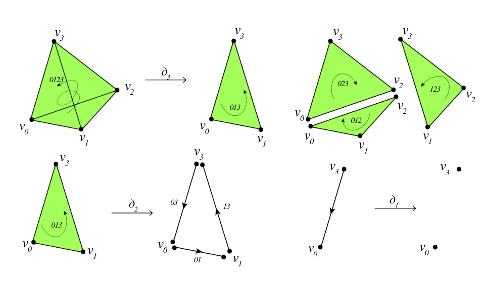
Figure 4: Examples of 1,2,31,2,3-boundary operators. For sake of brevity, we use 01230123 to represent a 33-simplex. 013,023,012,013,023,012, and 123123 to represent 22-simplices, and 01,13,01,13, and 0303 to represent 11-simplices. The 33-simplex 01230123 has a right-handed orientation. After the boundary map ∂3\partial_{3}, we have ∂3(0123)=123−023+013−012\partial_{3}(0123)=123-023+013-012. Two 22-simplices, 023023 and 012012, have opposite orientations as 123123 and 013013. Similarly, ∂2(013)=13−03+01\partial_{2}(013)=13-03+01, and ∂1(03)=3−0\partial_{1}(03)=3-0.

Let KK be an oriented simplicial complex, for integer q≥0q\geq 0, the qq-combinatorial Laplacian is a linear operator Δq:Cq​(K)⟶Cq​(K)\Delta_{q}:C_{q}(K)\longrightarrow C_{q}(K)

Δq:=∂q+1∂q+1∗+∂q∗∂q\Delta_{q}:=\partial_{q+1}\partial_{q+1}^{\ast}+\partial_{q}^{\ast}\partial_{q} (11)

with ∂q∂q+1=0\partial_{q}\partial_{q+1}=0, which implies Im(∂q+1)⊂ker(∂q)\text{Im}(\partial_{q+1})\subset\text{ker}(\partial_{q}). The qq-combinatorial Laplacian matrix, denoted ℒq\mathcal{L}_{q}, is the matrix representation22 2 If q=0q=0, ∂0\partial_{0} is a zero map, and we denote ℬ0\mathcal{B}_{0} a zero matrix with dimension 1×N1\times N, where NN is the number of 00-simplices. Note that this term is needed to attain the correct dimension of the null space. If q>dim​(K)q>\text{dim}(K), we will not discuss ∂q\partial_{q} since there is no σq\sigma_{q} in KK..

ℒq=ℬq+1​ℬq+1T+ℬqT​ℬq\mathcal{L}_{q}=\mathcal{B}_{q+1}\mathcal{B}_{q+1}^{T}+\mathcal{B}_{q}^{T}\mathcal{B}_{q} (12)

of operator Δq\Delta_{q}, with ℬq\mathcal{B}_{q} and ℬq+1\mathcal{B}_{q+1} being the matrices of dimension qq and q+1q+1. Additionally, we denote upper and lower qq-combinatorial Laplacian matrices by ℒqU=ℬq+1​ℬq+1T\mathcal{L}_{q}^{U}=\mathcal{B}_{q+1}\mathcal{B}_{q+1}^{T} and ℒqL=ℬqT​ℬq\mathcal{L}_{q}^{L}=\mathcal{B}_{q}^{T}\mathcal{B}_{q}, respectively. Note that ∂0\partial_{0} is the zero map which leads to ℬ0\mathcal{B}_{0} being a zero matrix. Therefore, ℒ0​(K)=ℬ1​ℬ1T+ℬ0T​ℬ0\mathcal{L}_{0}(K)=\mathcal{B}_{1}\mathcal{B}_{1}^{T}+\mathcal{B}_{0}^{T}\mathcal{B}_{0}, with KK the (oriented) simplicial complex of dimension 11, which is actually a simple graph. Especially, 00-combinatorial Laplacian matrix ℒ0​(K)\mathcal{L}_{0}(K) is actually the Laplacian matrix defined in the spectral graph theory. In fact, Eq. (2) is exactly the same as Eq. (16) given below.

Given an oriented simplicial complex KK with 0≤q≤dim​(K)0\leq q\leq\text{dim}(K), one can obtain the entries of its corresponding upper and lower qq-combinatorial Laplacian matrices explicitly [21]

(ℒqU)i​j\displaystyle(\mathcal{L}_{q}^{U})_{ij} ={degU​(σqi),if i=j,1,if i≠j, σqi∼Uσqj with similar orientation,−1,if i≠j, σqi∼Uσqj with dissimilar orientation,0,otherwise.\displaystyle=\begin{cases}\text{deg}_{U}(\sigma^{i}_{q}),&\mbox{if $i=j$,}\\ 1,&\mbox{if $i\neq j$, $\sigma^{i}_{q}\stackrel{{\scriptstyle U}}{{\sim}}\sigma^{j}_{q}$ with similar orientation,}\\ -1,&\mbox{if $i\neq j$, $\sigma^{i}_{q}\stackrel{{\scriptstyle U}}{{\sim}}\sigma^{j}_{q}$ with dissimilar orientation,}\\ 0,&\mbox{otherwise.}\end{cases} (13)
(ℒqL)i​j\displaystyle(\mathcal{L}_{q}^{L})_{ij} ={degL​(σqi)=q+1,if i=j,1,if i≠j, σqi∼Lσqj with similar orientation,−1,if i≠j, σqi∼Lσqj with dissimilar orientation,0,otherwise.\displaystyle=\begin{cases}\text{deg}_{L}(\sigma^{i}_{q})=q+1,&\mbox{if $i=j$,}\\ 1,&\mbox{if $i\neq j$, $\sigma^{i}_{q}\stackrel{{\scriptstyle L}}{{\sim}}\sigma^{j}_{q}$ with similar orientation,}\\ -1,&\mbox{if $i\neq j$, $\sigma^{i}_{q}\stackrel{{\scriptstyle L}}{{\sim}}\sigma^{j}_{q}$ with dissimilar orientation,}\\ 0,&\mbox{otherwise.}\end{cases} (14)

The entries of qq-combinatorial Laplacian matrices are

q>0,(ℒq)i​j\displaystyle q>0,\ (\mathcal{L}_{q})_{ij} ={deg​(σqi)+q+1,if i=j.1,if i≠j, σqi≁Uσqj and σqi∼Lσqj with similar orientation.−1,if i≠j, σqi≁Uσqj and σqi∼Lσqj with dissimilar orientation.0,if i≠j and either , σqi∼Uσqj or σqi≁Lσqj.\displaystyle=\begin{cases}\text{deg}(\sigma^{i}_{q})+q+1,&\mbox{if $i=j$.}\\ 1,&\mbox{if $i\neq j$, $\sigma^{i}_{q}\stackrel{{\scriptstyle U}}{{\nsim}}\sigma^{j}_{q}$ and $\sigma^{i}_{q}\stackrel{{\scriptstyle L}}{{\sim}}\sigma^{j}_{q}$ with similar orientation.}\\ -1,&\mbox{if $i\neq j$, $\sigma^{i}_{q}\stackrel{{\scriptstyle U}}{{\nsim}}\sigma^{j}_{q}$ and $\sigma^{i}_{q}\stackrel{{\scriptstyle L}}{{\sim}}\sigma^{j}_{q}$ with dissimilar orientation.}\\ 0,&\mbox{if $i\neq j$ and either , $\sigma^{i}_{q}\stackrel{{\scriptstyle U}}{{\sim}}\sigma^{j}_{q}$ or $\sigma^{i}_{q}\stackrel{{\scriptstyle L}}{{\nsim}}\sigma^{j}_{q}$.}\end{cases} (15)
q=0,(ℒq)i​j\displaystyle q=0,\ (\mathcal{L}_{q})_{ij} ={deg​(σ0i),if i=j.−1,if σ0i∼Uσ0j.0,otherwise.\displaystyle=\begin{cases}\text{deg}(\sigma^{i}_{0}),&\mbox{if $i=j$.}\\ -1,&\mbox{if $\sigma^{i}_{0}\stackrel{{\scriptstyle U}}{{\sim}}\sigma^{j}_{0}$.}\\ 0,&\mbox{otherwise.}\end{cases} (16)

2.3.2 Spectral analysis of qq-combinatorial Laplacian matrices

A qq-combinatorial Laplacian matrix for oriented simplicial complexes is a generalization of the Laplacian matrix in graph theory. The spectra of a Laplacian matrix play an essential role in understanding the connectivity and robustness of simple graphs (simplicial complexes of dimension 11). They can also distinguish different topological structures. Inspired by the capability of the Laplacian spectra of analyzing topological structures, we study the spectral properties of qq-combinatorial Laplacian matrices to reveal topological and spectral information of simplicial complexes with dimension 0≤q≤dim​(K)0\leq q\leq\text{dim}(K).

We clarify that for a given finite simplicial complex KK, the spectra of its qq-combinatorial Laplacian matrix is independent of the choice of the orientation for the qq-simplices of KK. The proof can be found in Ref. [21]. Figure 5 provides a simple example to illustrate this property. In Figure 5, we have two oriented simplicial complexes, K1K_{1} and K2K_{2}, with the same geometric structure but different orientations. For the sake of brevity, we use 1,2,3,4,1,2,3,4, and 55 to represent 00-simplices (vertices), 12,23,34,24,12,23,34,24, and 4545 to describe 11-simplices (edges), and 234234 to stand for the 22-simplex (triangle). Then the 00-combinatorial Laplacian matrix of K1K_{1} and K2K_{2} is

ℒ0​(K1)=ℒ0​(K2)=[1−1000−13−1−100−12−100−1−13−1000−11].\mathcal{L}_{0}(K_{1})=\mathcal{L}_{0}(K_{2})=\left[\begin{array}[]{ccccc}1&-1&0&0&0\\ -1&3&-1&-1&0\\ 0&-1&2&-1&0\\ 0&-1&-1&3&-1\\ 0&0&0&-1&1\end{array}\right].

Obviously, ℒ0​(K1)\mathcal{L}_{0}(K_{1}) and ℒ0​(K2)\mathcal{L}_{0}(K_{2}) have the same spectra. For q=1q=1, there are five 11-simplices in K1K_{1} and K2K_{2}, while 11-combinatorial Laplacian matrices have dimension 5×55\times 5. Using K1K_{1} as an example, since 1212 and 2323 are lower adjacent with similar orientation, the element of ℒ1​(K1)\mathcal{L}_{1}(K_{1}) addressed at first row and second column is 11 according to Eq. (15). Since 3434 and 4545 are lower adjacent with dissimilar orientation, (ℒ1​(K1))35=−1(\mathcal{L}_{1}(K_{1}))_{35}=-1. Moreover, 2323 and 3434 are upper adjacent which results in (ℒ1​(K1))23=0(\mathcal{L}_{1}(K_{1}))_{23}=0. For the diagonal parts, 1212 and 4545 are not the faces of any 22-simplex, while 23,34,23,34, and 2424 are the faces of 22-simplex 234234. Therefore, degU​(12)=degU​(12)=0\text{deg}_{U}(12)=\text{deg}_{U}(12)=0, and degU​(23)=degU​(34)=degU​(34)=1\text{deg}_{U}(23)=\text{deg}_{U}(34)=\text{deg}_{U}(34)=1, so the diagonal terms of ℒ0​(K1)\mathcal{L}_{0}(K_{1}) are 2,3,3,3,2,3,3,3, and 22.

ℒ1​(K1)=[21010130000030−11003−100−1−12],ℒ1​(K2)=[2−1010−13000003011003−1001−12].\mathcal{L}_{1}(K_{1})=\left[\begin{array}[]{ccccc}2&1&0&1&0\\ 1&3&0&0&0\\ 0&0&3&0&-1\\ 1&0&0&3&-1\\ 0&0&-1&-1&2\end{array}\right],\quad\mathcal{L}_{1}(K_{2})=\left[\begin{array}[]{ccccc}2&-1&0&1&0\\ -1&3&0&0&0\\ 0&0&3&0&1\\ 1&0&0&3&-1\\ 0&0&1&-1&2\end{array}\right].

The spectra of ℒ1​(K1)\mathcal{L}_{1}(K_{1}) and ℒ1​(K2)\mathcal{L}_{1}(K_{2}) have the same eigenvalues: {3,5±52,5±132}\{3,\dfrac{5\pm\sqrt{5}}{2},\dfrac{5\pm\sqrt{13}}{2}\}. Since K1K_{1} and K2K_{2} do not have 33-simplices, ℒq\mathcal{L}_{q} is a zero matrix when q≥3q\geq 3.

Refer to caption
Figure 5: Illustration of two oriented simplicial complexes with the same geometric structure but having different orientations. Here, we denote the vertices by 1,2,3,4,1,2,3,4, and 55, edges by 12,23,34,24,12,23,34,24, and 4545, and the triangle by 234234.

A qq-combinatorial Laplacian matrix is symmetric and positive semi-definite. Therefore, its eigenvalues are all real and non-negative. An analogy to the property that the number of zero eigenvalues of ℒ0\mathcal{L}_{0} represents the number of connected components (β0\beta_{0}) in the simple graph (simplicial complex with dimension 11), the number of zero eigenvalues of ℒq\mathcal{L}_{q} can also reveal the topological information. More specifically, for a given finite oriented simplicial complex, the Betti number βq{\beta_{q}} of KK satisfy

βq=dim​(ℒq​(K))−rank​(ℒq​(K))=nullity​(ℒq​(K))=#​of​zero​eigenvalues​of​ℒq​(K)\beta_{q}=\text{dim}(\mathcal{L}_{q}(K))-\text{rank}(\mathcal{L}_{q}(K))=\text{nullity}(\mathcal{L}_{q}(K))=\#~{\rm of~zero~eigenvalues~of}~\mathcal{L}_{q}(K) (17)

We consider tetrahedron-shaped structures in Figure 6 to illustrate the connection between Betti number and the dimension and the rank of qq-combinatorial Laplacian matrix. For the sake of brevity, we will use ii to represents 00-simplex [vi][v_{i}], i​jij to represents 11-simplex [vi,vj][v_{i},v_{j}], and i​j​kijk to represents [vi,vj,vk][v_{i},v_{j},v_{k}]. Then, 11- and 22-boundary operators map:

∂1(i​j)=j−i,∂2(i​j​k)=j​k−i​k+i​j,\begin{split}\partial_{1}(ij)&=j-i,\\ \partial_{2}(ijk)&=jk-ik+ij,\end{split}

Since different orientations result in the same spectrum, there is no need to label the orientation in Figure 6. In the following, we analyze three tetrahedron-shaped simplicial complexes:

Refer to caption
Figure 6: Illustration of three different tetrahedron-shaped simplicial complexes. There are four 00-simplices and six 11-simplices in K1K_{1}. Here, K2K_{2} has four more 22-simplices than K1K_{1} does, while K3K_{3} owns one more 33-simplex than K2K_{2} does.
  • 𝑲𝟏\bm{K_{1}}.

    The left most chart in Figure 6 has four 00-simplices: 0,1,2,0,1,2, and 3,3, and six 11-simplices: 01,02,03,12,13,01,02,03,12,13, and 2323. It is clear that Cq​(K1)C_{q}(K_{1}) is an empty set and ∂q\partial_{q} is an zero map when q≥2q\geq 2. Then, its Laplacian operators are

    Δ1=∂1∗∂1,Δ0=∂1∂1∗+∂0∗∂0.\Delta_{1}=\partial_{1}^{\ast}\partial_{1},\ \Delta_{0}=\partial_{1}\partial_{1}^{\ast}+\partial_{0}^{\ast}\partial_{0}.

    The combinatorial Laplacian matrices are:

    ℒ1=ℬ1T​ℬ1,ℒ0=ℬ1​ℬ1T+ℬ0T​ℬ0.\mathcal{L}_{1}=\mathcal{B}_{1}^{T}\mathcal{B}_{1},\ \mathcal{L}_{0}=\mathcal{B}_{1}\mathcal{B}_{1}^{T}+\mathcal{B}_{0}^{T}\mathcal{B}_{0}.

    The matrix representation ℬ1\mathcal{B}_{1} for ∂1:C1​(K1)⟶C0​(K1)\partial_{1}:C_{1}(K_{1})\longrightarrow C_{0}(K_{1}) is:

    ℬ1=0102031213230123[−1100−1010−10010−1100−10100−11].\mathcal{B}_{1}=\begin{array}[]{@{}r@{}c@{}c@{}c@{}c@{}c@{}c@{}l@{}}&01&02&03&12&13&23\\ \left.\begin{array}[]{c}0\\ 1\\ 2\\ 3\end{array}\right[&\begin{array}[]{c}-1\\ 1\\ 0\\ 0\end{array}&\begin{array}[]{c}-1\\ 0\\ 1\\ 0\end{array}&\begin{array}[]{c}-1\\ 0\\ 0\\ 1\end{array}&\begin{array}[]{c}0\\ -1\\ 1\\ 0\end{array}&\begin{array}[]{c}0\\ -1\\ 0\\ 1\end{array}&\begin{array}[]{c}0\\ 0\\ -1\\ 1\end{array}&\left].\begin{array}[]{c}\\ \\ \\ \\ \end{array}\right.\end{array} (18)

    and B0B_{0} is

    B0=0123[0000]B_{0}=\begin{array}[]{@{}r@{}c@{}c@{}c@{}c@{}l@{}}&0&1&2&3\\ \left.\begin{array}[]{c}\end{array}\right[&\begin{array}[]{c}0\end{array}&\begin{array}[]{c}0\end{array}&\begin{array}[]{c}0\end{array}&\begin{array}[]{c}0\end{array}&\left]\begin{array}[]{c}\end{array}\right.\end{array}

    Therefore, the associated combinatorial Laplacian matrices are

    ℒ1​(K1)=[211−1−1012110−1112011−11021−1−1011210−11−112],ℒ0​(K1)=[3−1−1−1−13−1−1−1−13−1−1−1−13].\mathcal{L}_{1}(K_{1})=\left[\begin{array}[]{cccccc}2&1&1&-1&-1&0\\ 1&2&1&1&0&-1\\ 1&1&2&0&1&1\\ -1&1&0&2&1&-1\\ -1&0&1&1&2&1\\ 0&-1&1&-1&1&2\end{array}\right],\ \mathcal{L}_{0}(K_{1})=\left[\begin{array}[]{cccc}3&-1&-1&-1\\ -1&3&-1&-1\\ -1&-1&3&-1\\ -1&-1&-1&3\end{array}\right].

    As shown in Table 3, we can calculate the spectra and ranks from combinatorial Laplacian matrices. We have β0=1\beta_{0}=1, β1=3\beta_{1}=3, which reveal that one connected component and three 11-cycles are exist in K1K_{1}.

    Table 3: Table of dimensions, ranks, nullity, spectra and Betti numbers of combinatorial Laplacian matrices ℒ0,\mathcal{L}_{0}, and ℒ1\mathcal{L}_{1} for simplicial complex K1K_{1}.
       ℒ1​(K1)\mathcal{L}_{1}(K_{1})       ℒ0​(K1)\mathcal{L}_{0}(K_{1})   
       Betti number       β1=3\beta_{1}=3       β0=1\beta_{0}=1   
       dim       66       44   
       rank       33       33   
       nullity       33       11   
       Spectra       {0,0,0,4,4,4}\{0,0,0,4,4,4\}       {0,4,4,4}\{0,4,4,4\}   
  • 𝑲𝟐\bm{K_{2}}.

    We analyze the middle chart in Figure 6 in a similar manner. As one can see, K2K_{2} has four 00-simplices: 0,1,2,0,1,2, and 33, six 11-simplices: 01,02,03,12,13,01,02,03,12,13, and 2323, and four 22-simplices: 012,013,023,012,013,023, and 123123. The associated Laplacian operators are

    Δ2=∂2∗∂2,Δ1=∂2∂2∗+∂1∗∂1,Δ0=∂1∂1∗+∂0∗∂0.\Delta_{2}=\partial_{2}^{\ast}\partial_{2},\ \Delta_{1}=\partial_{2}\partial_{2}^{\ast}+\partial_{1}^{\ast}\partial_{1},\ \Delta_{0}=\partial_{1}\partial_{1}^{\ast}+\partial_{0}^{\ast}\partial_{0}.

    The resulting combinatorial Laplacian matrices are

    ℒ2=ℬ2T​ℬ2,ℒ1=ℬ2​ℬ2T+ℬ1T​ℬ1,ℒ0=ℬ1​ℬ1T+ℬ0T​ℬ0.\mathcal{L}_{2}=\mathcal{B}_{2}^{T}\mathcal{B}_{2},\ \mathcal{L}_{1}=\mathcal{B}_{2}\mathcal{B}_{2}^{T}+\mathcal{B}_{1}^{T}\mathcal{B}_{1},\ \mathcal{L}_{0}=\mathcal{B}_{1}\mathcal{B}_{1}^{T}+\mathcal{B}_{0}^{T}\mathcal{B}_{0}.

    The corresponding matrix representations for ℬ2\mathcal{B}_{2} and ℬ1\mathcal{B}_{1} are respectively

    ℬ2=012013023123010203121323[1−1010010−101001−10010001−11],​ℬ1=0102031213230123[−1100−1010−10010−1100−10100−11].\mathcal{B}_{2}=\begin{array}[]{@{}r@{}c@{}c@{}c@{}c@{}l@{}}&012&013&023&123\\ \left.\begin{array}[]{c}01\\ 02\\ 03\\ 12\\ 13\\ 23\end{array}\right[&\begin{array}[]{c}1\\ -1\\ 0\\ 1\\ 0\\ 0\end{array}&\begin{array}[]{c}1\\ 0\\ -1\\ 0\\ 1\\ 0\end{array}&\begin{array}[]{c}0\\ 1\\ -1\\ 0\\ 0\\ 1\end{array}&\begin{array}[]{c}0\\ 0\\ 0\\ 1\\ -1\\ 1\end{array}&\left],\begin{array}[]{c}\\ \\ \\ \\ \\ \\ \end{array}\right.\end{array}\mathcal{B}_{1}=\begin{array}[]{@{}r@{}c@{}c@{}c@{}c@{}c@{}c@{}l@{}}&01&02&03&12&13&23\\ \left.\begin{array}[]{c}0\\ 1\\ 2\\ 3\end{array}\right[&\begin{array}[]{c}-1\\ 1\\ 0\\ 0\end{array}&\begin{array}[]{c}-1\\ 0\\ 1\\ 0\end{array}&\begin{array}[]{c}-1\\ 0\\ 0\\ 1\end{array}&\begin{array}[]{c}0\\ -1\\ 1\\ 0\end{array}&\begin{array}[]{c}0\\ -1\\ 0\\ 1\end{array}&\begin{array}[]{c}0\\ 0\\ -1\\ 1\end{array}&\left].\begin{array}[]{c}\\ \\ \\ \\ \end{array}\right.\end{array} (19)

    Then, associated combinatorial Laplacian matrices are

    ℒ2​(K2)=[31−11131−1−11311−113],ℒ1​(K2)=[400000040000004000000400000040000004],\mathcal{L}_{2}(K_{2})=\left[\begin{array}[]{cccc}3&1&-1&1\\ 1&3&1&-1\\ -1&1&3&1\\ 1&-1&1&3\end{array}\right],\ \mathcal{L}_{1}(K_{2})=\left[\begin{array}[]{cccccc}4&0&0&0&0&0\\ 0&4&0&0&0&0\\ 0&0&4&0&0&0\\ 0&0&0&4&0&0\\ 0&0&0&0&4&0\\ 0&0&0&0&0&4\end{array}\right],

    and ℒ0​(K2)=ℒ0​(K1)\mathcal{L}_{0}(K_{2})=\mathcal{L}_{0}(K_{1}). Similarly, from Table 4, we see that there are one connected component and one 22-cycle (void) in K2K_{2}.

    Table 4: Table of dimensions, ranks, nullity, spectra and Betti numbers of combinatorial Laplacian matrices ℒ0,ℒ1,\mathcal{L}_{0},\mathcal{L}_{1}, and ℒ2\mathcal{L}_{2} for simplicial complex K2K_{2}.
    ℒ2​(K2)\mathcal{L}_{2}(K_{2}) ℒ1​(K2)\mathcal{L}_{1}(K_{2}) ℒ0​(K2)\mathcal{L}_{0}(K_{2})
    Betti number β2=1\beta_{2}=1 β1=0\beta_{1}=0 β1=1\beta_{1}=1
    dim 44 66 44
    rank 33 66 33
    nullity 11 00 11
    Spectra {0,4,4,4}\{0,4,4,4\} {4,4,4,4,4,4}\{4,4,4,4,4,4\} {0,4,4,4}\{0,4,4,4\}
  • 𝑲𝟑\bm{K_{3}}.

    K3K_{3} in the right most chart in Figure 6 has four 00-simplices: 0,1,2,0,1,2, and 33, six 11-simplices: 01,02,03,12,13,01,02,03,12,13, and 2323, four 44-simplices: 012,013,023,012,013,023, and 123123, and one 33-simplex 0123401234. The associated Laplacian operators are

    Δ2=∂3∂3∗+∂2∗∂2,Δ1=∂2∂2∗+∂1∗∂1,Δ0=∂1∂1∗+∂0∗∂0.\Delta_{2}=\partial_{3}\partial_{3}^{\ast}+\partial_{2}^{\ast}\partial_{2},\ \Delta_{1}=\partial_{2}\partial_{2}^{\ast}+\partial_{1}^{\ast}\partial_{1},\ \Delta_{0}=\partial_{1}\partial_{1}^{\ast}+\partial_{0}^{\ast}\partial_{0}.

    The corresponding combinatorial Laplacian matrices are:

    ℒ2=ℬ3​ℬ3T+ℬ2T​ℬ2,ℒ1=ℬ2​ℬ2T+ℬ1T​ℬ1,ℒ0=ℬ1​ℬ1T+ℬ0T​ℬ0.\mathcal{L}_{2}=\mathcal{B}_{3}\mathcal{B}_{3}^{T}+\mathcal{B}_{2}^{T}\mathcal{B}_{2},\ \mathcal{L}_{1}=\mathcal{B}_{2}\mathcal{B}_{2}^{T}+\mathcal{B}_{1}^{T}\mathcal{B}_{1},\ \mathcal{L}_{0}=\mathcal{B}_{1}\mathcal{B}_{1}^{T}+\mathcal{B}_{0}^{T}\mathcal{B}_{0}.

    The resulting matrix representations ℬ1\mathcal{B}_{1} and ℬ2\mathcal{B}_{2} are exactly the same as those in Eq. (19). While ℬ3\mathcal{B}_{3} is given by

    ℬ3=0123012013023123[−11−11].\mathcal{B}_{3}=\begin{array}[]{@{}r@{}c@{}l@{}}&0123\\ \left.\begin{array}[]{c}012\\ 013\\ 023\\ 123\end{array}\right[&\begin{array}[]{c}-1\\ 1\\ -1\\ 1\end{array}&\left].\begin{array}[]{c}\\ \\ \\ \\ \end{array}\right.\end{array} (20)

    Therefore, the 22-combinatorial Laplacian matrices are

    ℒ2​(K3)=[4000040000400004],\mathcal{L}_{2}(K_{3})=\left[\begin{array}[]{cccc}4&0&0&0\\ 0&4&0&0\\ 0&0&4&0\\ 0&0&0&4\end{array}\right],

    ℒ1​(K3)=ℒ1​(K2)\mathcal{L}_{1}(K_{3})=\mathcal{L}_{1}(K_{2}), and ℒ0​(K3)=ℒ0​(K2)\mathcal{L}_{0}(K_{3})=\mathcal{L}_{0}(K_{2}). In this case, Table 5 shows that there is only one connected component in K3K_{3}, which matches the right most chart in Figure 6.

    Table 5: Table of dimensions, ranks, nullity, spectra and Betti numbers of combinatorial Laplacian matrices ℒ0,ℒ1,\mathcal{L}_{0},\mathcal{L}_{1}, and ℒ2\mathcal{L}_{2} for simplicial complex K3K_{3}.
    ℒ2​(K3)\mathcal{L}_{2}(K_{3}) ℒ1​(K3)\mathcal{L}_{1}(K_{3}) ℒ0​(K3)\mathcal{L}_{0}(K_{3})
    Betti number β2=0\beta_{2}=0 β1=0\beta_{1}=0 β0=1\beta_{0}=1
    dim 44 66 44
    rank 44 66 33
    nullity 00 00 11
    Spectra {4,4,4,4}\{4,4,4,4\} {4,4,4,4,4,4}\{4,4,4,4,4,4\} {0,4,4,4}\{0,4,4,4\}

2.3.3 Persistent spectral theory

Instead of using the aforementioned spectral analysis for qq-combinatorial Laplacian matrix to describe a single configuration, we propose a persistent spectral theory to create a sequence of simplicial complexes induced by varying a filtration parameter, which is inspired by persistent homology and our earlier work in multiscale graphs [44, 8].

A filtration of an oriented simplicial complex KK is a sequence of sub-complexes (Kt)t=0m(K_{t})_{t=0}^{m} of KK

∅=K0⊆K1⊆K2⊆⋯⊆Km=K.\emptyset=K_{0}\subseteq K_{1}\subseteq K_{2}\subseteq\cdots\subseteq K_{m}=K. (21)

It induces a sequence of chain complexes

⋯Cq+11⇌∂q+11∗∂q+11Cq1⇌∂q1∗∂q1⋯⇌∂31∗∂31C21⇌∂21∗∂21C11⇌∂11∗∂11C01⇌∂01∗∂01C−11⊆⊆⊆⊆⊆⋯Cq+12⇌∂q+12∗∂q+12Cq2⇌∂q2∗∂q2⋯⇌∂32∗∂32C22⇌∂22∗∂22C12⇌∂12∗∂12C02⇌∂02∗∂02C−11⊆⊆⊆⊆⊆⋯Cq+1m⇌∂q+1m∗∂q+1mCqm⇌∂qm∗∂qm⋯⇌∂3m∗∂3mC2m⇌∂2m∗∂2mC1m⇌∂1m∗∂1mC0m⇌∂0m∗∂0mC−11\left.\begin{array}[]{cccccccccccccc}\cdots&C_{q+1}^{1}&\xrightleftharpoons[\partial_{q+1}^{1^{\ast}}]{\partial_{q+1}^{1}}&C_{q}^{1}&\xrightleftharpoons[\partial_{q}^{1^{\ast}}]{\partial_{q}^{1}}&\cdots&\xrightleftharpoons[\partial_{3}^{1^{\ast}}]{\partial_{3}^{1}}&C_{2}^{1}&\xrightleftharpoons[\partial_{2}^{1^{\ast}}]{\partial_{2}^{1}}&C_{1}^{1}&\xrightleftharpoons[\partial_{1}^{1^{\ast}}]{\partial_{1}^{1}}&C_{0}^{1}&\xrightleftharpoons[\partial_{0}^{1^{\ast}}]{\partial_{0}^{1}}&C_{-1}^{1}\\ &\rotatebox{-90.0}{$\subseteq$}&&\rotatebox{-90.0}{$\subseteq$}&&&&\rotatebox{-90.0}{$\subseteq$}&&\rotatebox{-90.0}{$\subseteq$}&&\rotatebox{-90.0}{$\subseteq$}&&\\ \cdots&C_{q+1}^{2}&\xrightleftharpoons[\partial_{q+1}^{2^{\ast}}]{\partial_{q+1}^{2}}&C_{q}^{2}&\xrightleftharpoons[\partial_{q}^{2^{\ast}}]{\partial_{q}^{2}}&\cdots&\xrightleftharpoons[\partial_{3}^{2^{\ast}}]{\partial_{3}^{2}}&C_{2}^{2}&\xrightleftharpoons[\partial_{2}^{2^{\ast}}]{\partial_{2}^{2}}&C_{1}^{2}&\xrightleftharpoons[\partial_{1}^{2^{\ast}}]{\partial_{1}^{2}}&C_{0}^{2}&\xrightleftharpoons[\partial_{0}^{2^{\ast}}]{\partial_{0}^{2}}&C_{-1}^{1}\\ &\rotatebox{-90.0}{$\subseteq$}&&\rotatebox{-90.0}{$\subseteq$}&&&&\rotatebox{-90.0}{$\subseteq$}&&\rotatebox{-90.0}{$\subseteq$}&&\rotatebox{-90.0}{$\subseteq$}&&\\ \cdots&C_{q+1}^{m}&\xrightleftharpoons[\partial_{q+1}^{m^{\ast}}]{\partial_{q+1}^{m}}&C_{q}^{m}&\xrightleftharpoons[\partial_{q}^{m^{\ast}}]{\partial_{q}^{m}}&\cdots&\xrightleftharpoons[\partial_{3}^{m^{\ast}}]{\partial_{3}^{m}}&C_{2}^{m}&\xrightleftharpoons[\partial_{2}^{m^{\ast}}]{\partial_{2}^{m}}&C_{1}^{m}&\xrightleftharpoons[\partial_{1}^{m^{\ast}}]{\partial_{1}^{m}}&C_{0}^{m}&\xrightleftharpoons[\partial_{0}^{m^{\ast}}]{\partial_{0}^{m}}&C_{-1}^{1}\end{array}\right. (22)

where Cqt≔Cq​(Kt)C_{q}^{t}\coloneqq C_{q}(K_{t}) and ∂qt:Cq​(Kt)→Cq−1​(Kt)\partial_{q}^{t}\colon C_{q}(K_{t})\to C_{q-1}(K_{t}). Each KtK_{t} itself is an oriented simplicial complex which has dimension denoted by dim​(Kt)\text{dim}(K_{t}). If q<0q<0, then Cq​(Kt)={∅}C_{q}(K_{t})=\{\emptyset\} and ∂qt\partial_{q}^{t} is actually a zero map.33 3 We define the boundary matrix ℬ0t\mathcal{B}_{0}^{t} for boundary map ∂0t\partial_{0}^{t} as a zero matrix. The number of columns of ℬ0t\mathcal{B}_{0}^{t} is the number of 00-simplices in KtK_{t}, the number of rows will be 11. For a general case of 0<q≤dim​(Kt)0<q\leq\text{dim}(K_{t}), if σq\sigma_{q} is an oriented qq-simplex of KtK_{t}, then

∂qt(σq)=∑iq(−1)i​σq−1i,σq∈Kt,\partial_{q}^{t}(\sigma_{q})=\sum_{i}^{q}(-1)^{i}\sigma^{i}_{q-1},\sigma_{q}\in K_{t},

with σq=[v0,⋯,vq]\sigma_{q}=[v_{0},\cdots,v_{q}] being the oriented qq-simplex, and σq−1i=[v0,⋯,vi^,⋯,vq]\sigma^{i}_{q-1}=[v_{0},\cdots,\hat{v_{i}},\cdots,v_{q}] being the oriented (q−1)(q-1)-simplex for which its vertex viv_{i} is removed.

Let ℂqt+p\mathbb{C}_{q}^{t+p} be the subset of Cqt+pC_{q}^{t+p} whose boundary is in Cq−1tC_{q-1}^{t}:

ℂqt+p≔{α∈Cqt+p|∂qt+p(α)∈Cq−1t}.\mathbb{C}_{q}^{t+p}\coloneqq\{\alpha\in C_{q}^{t+p}\ |\ \partial_{q}^{t+p}(\alpha)\in C_{q-1}^{t}\}. (23)

We define

ðqt+p:ℂqt+p→Cq−1t\eth_{q}^{t+p}:\mathbb{C}_{q}^{t+p}\to C_{q-1}^{t} (24)

Based on the qq-combinatorial Laplacian operator, the p{p}-persistent q{q}-combinatorial Laplacian operator Δqt+p:Cq​(Kt)→Cq​(Kt)\Delta_{q}^{t+p}:C_{q}(K_{t})\to C_{q}(K_{t}) defined along the filtration can be expressed as

Δqt+p=ðq+1t+p(ðq+1t+p)∗+∂qt∗∂qt.\Delta_{q}^{t+p}=\eth_{q+1}^{t+p}\left(\eth_{q+1}^{t+p}\right)^{\ast}+\partial_{q}^{t^{\ast}}\partial_{q}^{t}. (25)

We denote the matrix representations of boundary operator ðq+1t+p\eth_{q+1}^{t+p} and ∂qt\partial_{q}^{t} by ℬq+1t+p\mathcal{B}_{q+1}^{t+p} and ℬqt\mathcal{B}_{q}^{t}, respectively. It is clear that the number of rows in ℬq+1t+p\mathcal{B}_{q+1}^{t+p} is the number of oriented qq-simplices in KtK_{t}, and the number of columns is the number of oriented (q+1)(q+1)-simplices in Kt+p∩ℂq+1t+pK_{t+p}\cap\mathbb{C}_{q+1}^{t+p}. The transpose of the matrices ℬq+1t+p\mathcal{B}_{q+1}^{t+p} and ℬqt\mathcal{B}_{q}^{t}, are the matrix representations of the adjoint boundary operator (∂q+1t+p)∗\left(\partial_{q+1}^{t+p}\right)^{\ast} and ∂qt∗\partial_{q}^{t^{\ast}}, respectively. Therefore, the p{p}-persistent q{q}-combinatorial Laplacian matrix, ℒqt+p\mathcal{L}_{q}^{t+p}, is

ℒqt+p=ℬq+1t+p​(ℬq+1t+p)T+(ℬqt)T​ℬqt.\mathcal{L}_{q}^{t+p}=\mathcal{B}_{q+1}^{t+p}(\mathcal{B}_{q+1}^{t+p})^{T}+(\mathcal{B}_{q}^{t})^{T}\mathcal{B}_{q}^{t}. (26)

Intuitively, for a non-empty set CqtC_{q}^{t}, the pp-persistent qq-combinatorial Laplacian matrix ℒqt+p\mathcal{L}_{q}^{t+p} is a square matrix with dimension to be the number of qq-simplices in KtK_{t}. Moreover, ℒqt+p\mathcal{L}_{q}^{t+p} is symmetric and positive semi-defined and thus, all the spectra of ℒqt+p\mathcal{L}_{q}^{t+p} are real and non-negative. If p=0p=0, then ℒqt+0\mathcal{L}_{q}^{t+0} is exactly the qq-combinatorial Laplacian matrix defined in Eq. (12).

We are interested in the difference between ℒqt+0\mathcal{L}_{q}^{t+0} and ℒqt+p\mathcal{L}_{q}^{t+p}. Suppose we have an oriented simplicial complex KtK_{t}, and also an oriented simplicial complex Kt+pK_{t+p} constructed by adding different dimensions simplices (”outer” topological structures) to KtK_{t} with dim​(Kt+p)=q+1\text{dim}(K_{t+p})=q+1. Since Kt⊂Kt+pK_{t}\subset K_{t+p}, we have

ℒqt+0=ℬq+1t+0​(ℬq+1t+0)T+(ℬqt)T​ℬqtℒqt+p=ℬq+1t+p​(ℬq+1t+p)T+(ℬqt)T​ℬqt.\begin{split}\mathcal{L}_{q}^{t+0}&=\mathcal{B}_{q+1}^{t+0}(\mathcal{B}_{q+1}^{t+0})^{T}+(\mathcal{B}_{q}^{t})^{T}\mathcal{B}_{q}^{t}\\ \mathcal{L}_{q}^{t+p}&=\mathcal{B}_{q+1}^{t+p}(\mathcal{B}_{q+1}^{t+p})^{T}+(\mathcal{B}_{q}^{t})^{T}\mathcal{B}_{q}^{t}.\end{split}
  1. Case 1

    . If (Im​(ðq+1t+p)∩(Kt+p\Kt))∩Cqt=∅(\text{Im}(\eth_{q+1}^{t+p})\cap(K_{t+p}\backslash K_{t}))\cap C_{q}^{t}=\emptyset for all possible qq, then the ”outer” topological structures are disconnected with KtK_{t}. Therefore, the boundary matrix ℬq+1t+p\mathcal{B}_{q+1}^{t+p} will add at least one additional zero column, which leads to at least one additional zero row for (ℬq+1t+p)T(\mathcal{B}_{q+1}^{t+p})^{T}. However, the matrix obtained by ℬq+1t+p​(ℬq+1t+p)T\mathcal{B}_{q+1}^{t+p}(\mathcal{B}_{q+1}^{t+p})^{T} does not change and ℒqt+p\mathcal{L}_{q}^{t+p} is exactly the same as ℒqt+0\mathcal{L}_{q}^{t+0}. In this situation, the spectra of ℒqt+0\mathcal{L}_{q}^{t+0} and ℒqt+p\mathcal{L}_{q}^{t+p} are exactly the same, which reveals the fact that the topological structure KtK_{t} does not change under the filtration process.

  2. Case 2

    . If (Im​(ðq+1t+p)∩(Kt+p\Kt))∩Cqt≠∅(\text{Im}(\eth_{q+1}^{t+p})\cap(K_{t+p}\backslash K_{t}))\cap C_{q}^{t}\neq\emptyset for at least one qq, then the boundary matrix ℬq+1t+p\mathcal{B}_{q+1}^{t+p} will be changed by adding additional non-zero columns. Therefore, ℒqt+p\mathcal{L}_{q}^{t+p} is no longer the same as ℒqt+0\mathcal{L}_{q}^{t+0}, but the structure information in KtK_{t} will still be preserved in ℒqt+p\mathcal{L}_{q}^{t+p}. In this case, the topological structure KtK_{t} builds connection with “outer” topological structures. By calculating the spectra of ℒqt+p\mathcal{L}_{q}^{t+p}, the disappeared and preserved structure information of KtK_{t} under the filtration process can be revealed.

Based on the fact that the topological and spectral information of KtK_{t} can also be analyzed from ℒq​(Kt)\mathcal{L}_{q}(K_{t}) along with the filtration parameter by diagonalizing the qq-combinatorial Laplacian matrix, we focus on the spectra information calculated from ℒqt+p\mathcal{L}_{q}^{t+p}. Denote the set of spectra of ℒqt+p\mathcal{L}_{q}^{t+p} by

Spectra​(ℒqt+p)={(λ1)qt+p,(λ2)qt+p,⋯,(λN)qt+p},\text{Spectra}(\mathcal{L}_{q}^{t+p})=\{(\lambda_{1})_{q}^{t+p},(\lambda_{2})_{q}^{t+p},\cdots,(\lambda_{N})_{q}^{t+p}\},

where ℒqt+p\mathcal{L}_{q}^{t+p} has dimension N×NN\times N and spectra are arranged in ascending order. The smallest non-zero eigenvalue of ℒqt+p\mathcal{L}_{q}^{t+p} is defined as (λ~2)qt+p(\tilde{\lambda}_{2})_{q}^{t+p}. In the previous section, we have seen that Betti numbers (i.e #\# of zero eigenvalues) can reveal qq-cycle information. Similarly, we define the number of zero eigenvalues of pp-persistent qq-combinatorial Laplacian matrix ℒqt+p\mathcal{L}_{q}^{t+p} to be the p{p}-persistent q{q}th Betti numbers

βqt+p=dim​(ℒqt+p)−rank​(ℒqt+p)=nullity​(ℒqt+p)=#​of​zero​eigenvalues​of​ℒqt+p.\beta_{q}^{t+p}=\text{dim}(\mathcal{L}_{q}^{t+p})-\text{rank}(\mathcal{L}_{q}^{t+p})=\text{nullity}(\mathcal{L}_{q}^{t+p})=\bm{\#}~{\rm of~zero~eigenvalues~of~}\mathcal{L}_{q}^{t+p}. (27)

In fact, βqt+p\beta_{q}^{t+p} counts the number of qq-cycles in KtK_{t} that are still alive in Kt+pK_{t+p}, which exactly provides the same topological information as persistent homology does. However, persistent spectral theory offers additional geometric information from the spectra of persistent combinatorial Laplacian matrix beyond topological persistence. In general, the topological changes can be read off from persistent Betti numbers (harmonic persistent spectra) and the geometric changes can be derived from the non-harmonic persistent spectra.

Figure 7demonstrates an example of a standard filtration process. Here the initial setup K1K_{1} consists of five 00-simplices (vertices). We construct Vietoris–Rips complexes by using an ever-growing circle centered at each vertex with radius rr. Once two circles overlapped with each other, an 11-simplex (edge) is formed. A 22-simplex (triangle) will be created when 33 circles contact with one another, and a 33-simplex will be generated once 44 circles get overlapped one another. As Figure 7 shows, we can attain a series of simplicial complexes from K1K_{1} to K6K_{6} with the radius of circles increasing. To fully illustrate how to construct pp-persistent qq-combinatorial Laplacian matrices by the boundary operator and determine persistent Betti numbers, we analyze 66 pp-persistent qq-combinatorial Laplacian matrices and their corresponding harmonic persistent spectra (i.e., persistent Betti numbers) and non-harmonic persistent spectra. Additional matrices are analyzed in Appendix Appendix B.

Refer to caption
Figure 7: Illustration of filtration. We use 0,1,2,3,0,1,2,3, and 44 to stand for 00-simplices, 01,12,23,03,24,02,01,12,23,03,24,02, and 1313 for 11-simplices, 012,023,013,012,023,013, and 123123 for 22-simplices, and 01230123 for the 33-simplex. Here, K1K_{1} has five 0-cycles, K2K_{2} has four 0-cycles, K3K_{3} has two 00-cycles and a 11-cycle, K4K_{4} has a 00-cycle and a 11-cycle, K5K_{5} has one 00-cycle, and K6K_{6} has a 00-cycle.
Table 6: The number of qq-cycles of simplicial complexes demonstrated in Figure 7.
#\# of qq-cycles K1K_{1} K2K_{2} K3K_{3} K4K_{4} K5K_{5} K6K_{6}
q=0q=0 55 44 22 11 11 11
q=1q=1 00 00 11 11 00 00
q=2q=2 00 00 00 00 00 00
  1. Case 11.

    In this case, the initial setup is K1K_{1} and the end status is K3K_{3}. Therefore, t=1t=1 and p=2p=2 in Eq. (26). We will calculate ℒ01+2,ℒ11+2,\mathcal{L}_{0}^{1+2},\mathcal{L}_{1}^{1+2}, and ℒ21+2\mathcal{L}_{2}^{1+2} first and find out their corresponding persistent spectra.

    The 22-persistent 0,1,20,1,2-combinatorial Laplacian operators are:

    Δ01+2=ð11+2(ð11+2)∗+∂01∗∂01,Δ11+2=ð21+2(ð21+2)∗+∂11∗∂11,Δ21+2=ð31+2(ð31+2)∗+∂21∗∂21,\begin{split}\Delta_{0}^{1+2}&=\eth_{1}^{1+2}\left(\eth_{1}^{1+2}\right)^{\ast}+\partial_{0}^{1^{\ast}}\partial_{0}^{1},\\ \Delta_{1}^{1+2}&=\eth_{2}^{1+2}\left(\eth_{2}^{1+2}\right)^{\ast}+\partial_{1}^{1^{\ast}}\partial_{1}^{1},\\ \Delta_{2}^{1+2}&=\eth_{3}^{1+2}\left(\eth_{3}^{1+2}\right)^{\ast}+\partial_{2}^{1^{\ast}}\partial_{2}^{1},\end{split}

    Since 22-simplex and 33-simplex do not exist in K1K_{1} and K3K_{3}, ð21+2,∂11,ð31+2,\eth_{2}^{1+2},\partial_{1}^{1},\eth_{3}^{1+2}, and ∂21\partial_{2}^{1} do not exist and ∂01\partial_{0}^{1} is a zero map. Then, there is only one persistent combinatorial Laplacian matrix

    ℒ01+2=ℬ11+2​(ℬ11+2)T+(ℬ01)T​ℬ01.\mathcal{L}_{0}^{1+2}=\mathcal{B}_{1}^{1+2}(\mathcal{B}_{1}^{1+2})^{T}+(\mathcal{B}_{0}^{1})^{T}\mathcal{B}_{0}^{1}.

    It can be seen in Figure 7 that two 00-cycles (connected components) in K1K_{1} are still alive in K3K_{3}, while no 11-cycle and 22-cycle exist in the initial set up K1K_{1}, which perfectly match the calculations in Table 7: β01+2=2\beta_{0}^{1+2}=2.

    Table 7: K1→K3K_{1}\to K_{3}
    qq q=0q=0 q=1q=1 q=2q=2
    ℬq+11+2\mathcal{B}_{q+1}^{1+2} 0112230301234[−110000−110000−110−10010]\begin{array}[]{@{}r@{}c@{}c@{}c@{}c@{}l@{}}&01&12&23&03\\ \left.\begin{array}[]{c}0\\ 1\\ 2\\ 3\\ 4\end{array}\right[&\begin{array}[]{c}-1\\ 1\\ 0\\ 0\\ 0\end{array}&\begin{array}[]{c}0\\ -1\\ 1\\ 0\\ 0\end{array}&\begin{array}[]{c}0\\ 0\\ -1\\ 1\\ 0\end{array}&\begin{array}[]{c}-1\\ 0\\ 0\\ 1\\ 0\end{array}&\left]\begin{array}[]{c}\\ \\ \\ \\ \\ \end{array}\right.\end{array} / /
    ℬq1\mathcal{B}_{q}^{1} 01234/[00000]\begin{array}[]{@{}r@{}c@{}c@{}c@{}c@{}c@{}l@{}}&0&1&2&3&4\\ \left.\begin{array}[]{c}/\end{array}\right[&\begin{array}[]{c}0\end{array}&\begin{array}[]{c}0\end{array}&\begin{array}[]{c}0\end{array}&\begin{array}[]{c}0\end{array}&\begin{array}[]{c}0\end{array}&\left]\begin{array}[]{c}\\ \end{array}\right.\end{array} / /
    ℒq1+2\mathcal{L}_{q}^{1+2} [2−10−10−12−1000−12−10−10−12000000]\left[\begin{array}[]{ccccc}2&-1&0&-1&0\\ -1&2&-1&0&0\\ 0&-1&2&-1&0\\ -1&0&-1&2&0\\ 0&0&0&0&0\end{array}\right] / /
    βq1+2\beta_{q}^{1+2} 2 / /
    dim​(ℒq1+2)\text{dim}(\mathcal{L}_{q}^{1+2}) 5 / /
    rank​(ℒq1+2)\text{rank}(\mathcal{L}_{q}^{1+2}) 3 / /
    nullity​(ℒq1+2)\text{nullity}(\mathcal{L}_{q}^{1+2}) 2 / /
    Spectrum​(ℒq1+2)\text{Spectrum}(\mathcal{L}_{q}^{1+2}) {0,0,2,2,4}\{0,0,2,2,4\} / /

  2. Case 22.

    The initial setup is K3K_{3} and the end status is K4K_{4}. The 11-persistent 0,1,20,1,2-combinatorial Laplacian operators are

    Δ03+1=ð13+1(ð13+1)∗+∂03∗∂03,Δ13+1=ð23+1​(ð23+1)∗+∂13∗∂13,Δ23+1=ð33+1(ð33+1)∗+∂23∗∂23,\begin{split}\Delta_{0}^{3+1}&=\eth_{1}^{3+1}\left(\eth_{1}^{3+1}\right)^{\ast}+\partial_{0}^{3^{\ast}}\partial_{0}^{3},\\ \Delta_{1}^{3+1}&=\eth_{2}^{3+1}\left(\eth_{2}^{3+1}\right)^{\ast}+\partial_{1}^{3^{\ast}}\partial 1^{3},\\ \Delta_{2}^{3+1}&=\eth_{3}^{3+1}\left(\eth_{3}^{3+1}\right)^{\ast}+\partial_{2}^{3^{\ast}}\partial_{2}^{3},\\ \end{split}

    Since 22-simplex and 33-simplex do not exist in K4K_{4}, ∂23,∂23+1,\partial_{2}^{3},\partial_{2}^{3+1}, and ∂23\partial_{2}^{3} do not exist, then

    ℒ03+1=ℬ13+1​(ℬ13+1)T+(ℬ03)T​ℬ03,ℒ13+1=(ℬ13)T​ℬ13.\begin{split}\mathcal{L}_{0}^{3+1}&=\mathcal{B}_{1}^{3+1}\left(\mathcal{B}_{1}^{3+1}\right)^{T}+(\mathcal{B}_{0}^{3})^{T}\mathcal{B}_{0}^{3},\\ \mathcal{L}_{1}^{3+1}&=(\mathcal{B}_{1}^{3})^{T}\mathcal{B}_{1}^{3}.\end{split}

    From Table 8, one can see that β03+1=0\beta_{0}^{3+1}=0 and β13+1=1\beta_{1}^{3+1}=1, which reveals only one 00-cycle and one 11-cycle in K3K_{3} are still alive in K4K_{4}.

    Table 8: K3→K4K_{3}\to K_{4}
    qq q=0q=0 q=1q=1 q=2q=2
    ℬq+13+1\mathcal{B}_{q+1}^{3+1} 011223032401234[−110000−110000−110−1001000−101]\begin{array}[]{@{}r@{}c@{}c@{}c@{}c@{}c@{}l@{}}&01&12&23&03&24\\ \left.\begin{array}[]{c}0\\ 1\\ 2\\ 3\\ 4\end{array}\right[&\begin{array}[]{c}-1\\ 1\\ 0\\ 0\\ 0\end{array}&\begin{array}[]{c}0\\ -1\\ 1\\ 0\\ 0\end{array}&\begin{array}[]{c}0\\ 0\\ -1\\ 1\\ 0\end{array}&\begin{array}[]{c}-1\\ 0\\ 0\\ 1\\ 0\end{array}&\begin{array}[]{c}0\\ 0\\ -1\\ 0\\ 1\end{array}&\left]\begin{array}[]{c}\\ \\ \\ \\ \\ \end{array}\right.\end{array} / /
    ℬq3\mathcal{B}_{q}^{3} 01234[00000]\begin{array}[]{@{}r@{}c@{}c@{}c@{}c@{}c@{}l@{}}&0&1&2&3&4\\ \left.\begin{array}[]{c}\end{array}\right[&\begin{array}[]{c}0\end{array}&\begin{array}[]{c}0\end{array}&\begin{array}[]{c}0\end{array}&\begin{array}[]{c}0\end{array}&\begin{array}[]{c}0\end{array}&\left]\begin{array}[]{c}\end{array}\right.\end{array} 0112230301234[−110000−110000−110−10010]\begin{array}[]{@{}r@{}c@{}c@{}c@{}c@{}l@{}}&01&12&23&03\\ \left.\begin{array}[]{c}0\\ 1\\ 2\\ 3\\ 4\end{array}\right[&\begin{array}[]{c}-1\\ 1\\ 0\\ 0\\ 0\end{array}&\begin{array}[]{c}0\\ -1\\ 1\\ 0\\ 0\end{array}&\begin{array}[]{c}0\\ 0\\ -1\\ 1\\ 0\end{array}&\begin{array}[]{c}-1\\ 0\\ 0\\ 1\\ 0\end{array}&\left]\begin{array}[]{c}\\ \\ \\ \\ \\ \end{array}\right.\end{array} /
    ℒq3+1\mathcal{L}_{q}^{3+1} [2−10−10−12−1000−13−1−1−10−12000−101]\left[\begin{array}[]{ccccc}2&-1&0&-1&0\\ -1&2&-1&0&0\\ 0&-1&3&-1&-1\\ -1&0&-1&2&0\\ 0&0&-1&0&1\end{array}\right] [2−101−12−100−1211012]\left[\begin{array}[]{cccc}2&-1&0&1\\ -1&2&-1&0\\ 0&-1&2&1\\ 1&0&1&2\\ \end{array}\right] /
    βq3+1\beta_{q}^{3+1} 1 1 /
    dim​(ℒq3+1)\text{dim}(\mathcal{L}_{q}^{3+1}) 5 4 /
    rank​(ℒq3+1)\text{rank}(\mathcal{L}_{q}^{3+1}) 4 3 /
    nullity​(ℒq3+1)\text{nullity}(\mathcal{L}_{q}^{3+1}) 1 1 /
    Spectra​(ℒq3+1)\text{Spectra}(\mathcal{L}_{q}^{3+1}) {0,0.8299,2,2.6889,4.4812}\{0,0.8299,2,2.6889,4.4812\} {0,2,2,4}\{0,2,2,4\} /

  3. Case 33.

    The initial setup is K4K_{4} and the end status is K4K_{4}. Similarly,

    ℒ04+0=ℬ14+0​(ℬ14+0)T+(ℬ04)T​ℬ04,ℒ14+0=(ℬ14)T​ℬ14,\begin{split}\mathcal{L}_{0}^{4+0}&=\mathcal{B}_{1}^{4+0}\left(\mathcal{B}_{1}^{4+0}\right)^{T}+(\mathcal{B}_{0}^{4})^{T}\mathcal{B}_{0}^{4},\\ \mathcal{L}_{1}^{4+0}&=(\mathcal{B}_{1}^{4})^{T}\mathcal{B}_{1}^{4},\end{split}

    and ℒ24+0\mathcal{L}_{2}^{4+0} does not exist. In this case, the 00-persistent qq-combinatorial Laplacian matrix is actually the qq-combinatorial Laplacian matrix defined in Eq. (12). Therefore, β04+0,β14+0,\beta_{0}^{4+0},\beta_{1}^{4+0}, and β24+0\beta_{2}^{4+0} actually represent the number of 0,1,20,1,2-cycles in K4K_{4}. With the filtration parameter rr increasing, all the circles overlapped with at least another circle in K4K_{4}, which results in β04+0=1\beta_{0}^{4+0}=1. Since only one 11-cycle formed in K4K_{4}, one has β14+0=1\beta_{1}^{4+0}=1.

    Table 9: K4→K4K_{4}\to K_{4}
    qq q=0q=0 q=1q=1 q=2q=2
    ℬq+14+0\mathcal{B}_{q+1}^{4+0} 011223032401234[−110000−110000−110−1001000−101]\begin{array}[]{@{}r@{}c@{}c@{}c@{}c@{}c@{}l@{}}&01&12&23&03&24\\ \left.\begin{array}[]{c}0\\ 1\\ 2\\ 3\\ 4\end{array}\right[&\begin{array}[]{c}-1\\ 1\\ 0\\ 0\\ 0\end{array}&\begin{array}[]{c}0\\ -1\\ 1\\ 0\\ 0\end{array}&\begin{array}[]{c}0\\ 0\\ -1\\ 1\\ 0\end{array}&\begin{array}[]{c}-1\\ 0\\ 0\\ 1\\ 0\end{array}&\begin{array}[]{c}0\\ 0\\ -1\\ 0\\ 1\end{array}&\left]\begin{array}[]{c}\\ \\ \\ \\ \\ \end{array}\right.\end{array} / /
    ℬq4\mathcal{B}_{q}^{4} 01234/[00000]\begin{array}[]{@{}r@{}c@{}c@{}c@{}c@{}c@{}l@{}}&0&1&2&3&4\\ \left.\begin{array}[]{c}/\end{array}\right[&\begin{array}[]{c}0\end{array}&\begin{array}[]{c}0\end{array}&\begin{array}[]{c}0\end{array}&\begin{array}[]{c}0\end{array}&\begin{array}[]{c}0\end{array}&\left]\begin{array}[]{c}\\ \end{array}\right.\end{array} 011223032401234[−110000−110000−110−1001000−101]\begin{array}[]{@{}r@{}c@{}c@{}c@{}c@{}c@{}l@{}}&01&12&23&03&24\\ \left.\begin{array}[]{c}0\\ 1\\ 2\\ 3\\ 4\end{array}\right[&\begin{array}[]{c}-1\\ 1\\ 0\\ 0\\ 0\end{array}&\begin{array}[]{c}0\\ -1\\ 1\\ 0\\ 0\end{array}&\begin{array}[]{c}0\\ 0\\ -1\\ 1\\ 0\end{array}&\begin{array}[]{c}-1\\ 0\\ 0\\ 1\\ 0\end{array}&\begin{array}[]{c}0\\ 0\\ -1\\ 0\\ 1\end{array}&\left]\begin{array}[]{c}\\ \\ \\ \\ \\ \end{array}\right.\end{array} /
    ℒq4+0\mathcal{L}_{q}^{4+0} [2−10−10−12−1000−13−1−1−10−12000−101]\left[\begin{array}[]{ccccc}2&-1&0&-1&0\\ -1&2&-1&0&0\\ 0&-1&3&-1&-1\\ -1&0&-1&2&0\\ 0&0&-1&0&1\end{array}\right] [2−1010−12−10−10−1211101200−1102]\left[\begin{array}[]{ccccc}2&-1&0&1&0\\ -1&2&-1&0&-1\\ 0&-1&2&1&1\\ 1&0&1&2&0\\ 0&-1&1&0&2\end{array}\right] /
    βq4+0\beta_{q}^{4+0} 1 1 /
    dim​(ℒq4+0)\text{dim}(\mathcal{L}_{q}^{4+0}) 5 5 /
    rank​(ℒq4+0)\text{rank}(\mathcal{L}_{q}^{4+0}) 4 4 /
    nullity​(ℒq4+0)\text{nullity}(\mathcal{L}_{q}^{4+0}) 1 1 /
    Spectra​(ℒq4+0)\text{Spectra}(\mathcal{L}_{q}^{4+0}) {0,0.8299,2,2.6889,4.4812}\{0,0.8299,2,2.6889,4.4812\} {0,0.8299,2,2.6889,4.4812}\{0,0.8299,2,2.6889,4.4812\} /

  4. Case 44.

    The initial setup is K4K_{4} and the end status is K5K_{5}. Using similar analysis as in previous cases, we have

    ℒ04+1=ℬ14+1​(ℬ14+1)T+(ℬ04)T​ℬ04,ℒ14+1=ℬ24+1​(ℬ24+1)T+(ℬ14)T​ℬ14,\begin{split}\mathcal{L}_{0}^{4+1}&=\mathcal{B}_{1}^{4+1}\left(\mathcal{B}_{1}^{4+1}\right)^{T}+(\mathcal{B}_{0}^{4})^{T}\mathcal{B}_{0}^{4},\\ \mathcal{L}_{1}^{4+1}&=\mathcal{B}_{2}^{4+1}\left(\mathcal{B}_{2}^{4+1}\right)^{T}+(\mathcal{B}_{1}^{4})^{T}\mathcal{B}_{1}^{4},\end{split}

    and ℒ24+1\mathcal{L}_{2}^{4+1} does not exist. Notice that two 22-simplices 012012 and 023023 are created under the filtration process. The appearance of these two newborns results in the 11-cycle that was alive in K4K_{4} being killed. Therefore β14+1=0\beta_{1}^{4+1}=0 and β04+1=1\beta_{0}^{4+1}=1 because only one connected component keeps alive until K5K_{5}.

    Table 10: K4→K5K_{4}\to K_{5}
    qq q=0q=0 q=1q=1 q=2q=2
    ℬq+14+1\mathcal{B}_{q+1}^{4+1} 01122303240201234[−110000−110000−110−1001000−101−10100]\begin{array}[]{@{}r@{}c@{}c@{}c@{}c@{}c@{}c@{}l@{}}&01&12&23&03&24&02\\ \left.\begin{array}[]{c}0\\ 1\\ 2\\ 3\\ 4\end{array}\right[&\begin{array}[]{c}-1\\ 1\\ 0\\ 0\\ 0\end{array}&\begin{array}[]{c}0\\ -1\\ 1\\ 0\\ 0\end{array}&\begin{array}[]{c}0\\ 0\\ -1\\ 1\\ 0\end{array}&\begin{array}[]{c}-1\\ 0\\ 0\\ 1\\ 0\end{array}&\begin{array}[]{c}0\\ 0\\ -1\\ 0\\ 1\end{array}&\begin{array}[]{c}-1\\ 0\\ 1\\ 0\\ 0\end{array}&\left]\begin{array}[]{c}\\ \\ \\ \\ \\ \end{array}\right.\end{array} 0120230112230324[11000001−10]\begin{array}[]{@{}r@{}c@{}c@{}l@{}}&012&023\\ \left.\begin{array}[]{c}01\\ 12\\ 23\\ 03\\ 24\end{array}\right[&\begin{array}[]{c}1\\ 1\\ 0\\ 0\\ 0\end{array}&\begin{array}[]{c}0\\ 0\\ 1\\ -1\\ 0\end{array}&\left]\begin{array}[]{c}\\ \\ \\ \\ \\ \end{array}\right.\end{array} /
    ℬq4\mathcal{B}_{q}^{4} 01234/[00000]\begin{array}[]{@{}r@{}c@{}c@{}c@{}c@{}c@{}l@{}}&0&1&2&3&4\\ \left.\begin{array}[]{c}/\end{array}\right[&\begin{array}[]{c}0\end{array}&\begin{array}[]{c}0\end{array}&\begin{array}[]{c}0\end{array}&\begin{array}[]{c}0\end{array}&\begin{array}[]{c}0\end{array}&\left]\begin{array}[]{c}\\ \end{array}\right.\end{array} 011223032401234[−110000−110000−110−1001000−101]\begin{array}[]{@{}r@{}c@{}c@{}c@{}c@{}c@{}l@{}}&01&12&23&03&24\\ \left.\begin{array}[]{c}0\\ 1\\ 2\\ 3\\ 4\end{array}\right[&\begin{array}[]{c}-1\\ 1\\ 0\\ 0\\ 0\end{array}&\begin{array}[]{c}0\\ -1\\ 1\\ 0\\ 0\end{array}&\begin{array}[]{c}0\\ 0\\ -1\\ 1\\ 0\end{array}&\begin{array}[]{c}-1\\ 0\\ 0\\ 1\\ 0\end{array}&\begin{array}[]{c}0\\ 0\\ -1\\ 0\\ 1\end{array}&\left]\begin{array}[]{c}\\ \\ \\ \\ \\ \end{array}\right.\end{array} /
    ℒq4+1\mathcal{L}_{q}^{4+1} [3−1−1−10−12−100−1−14−1−1−10−12000−101]\left[\begin{array}[]{ccccc}3&-1&-1&-1&0\\ -1&2&-1&0&0\\ -1&-1&4&-1&-1\\ -1&0&-1&2&0\\ 0&0&-1&0&1\end{array}\right] [3001003−10−10−1301100300−1102]\left[\begin{array}[]{ccccc}3&0&0&1&0\\ 0&3&-1&0&-1\\ 0&-1&3&0&1\\ 1&0&0&3&0\\ 0&-1&1&0&2\end{array}\right] /
    βq4+1\beta_{q}^{4+1} 1 0 /
    dim​(ℒq4+1)\text{dim}(\mathcal{L}_{q}^{4+1}) 5 5 /
    rank​(ℒq4+1)\text{rank}(\mathcal{L}_{q}^{4+1}) 4 5 /
    nullity​(ℒq4+1)\text{nullity}(\mathcal{L}_{q}^{4+1}) 1 0 /
    Spectra​(ℒq4+1)\text{Spectra}(\mathcal{L}_{q}^{4+1}) {0,1,2,4,5}\{0,1,2,4,5\} {1.2677,2,2,4,4.7321}\{1.2677,2,2,4,4.7321\} /

  5. Case 55.

    The initial setup is K5K_{5} and the end status is K6K_{6}. The 11-persistent 0,1,20,1,2-combinatorial Laplacian matrices are

    ℒ05+1=ℬ15+1​(ℬ15+1)T+(ℬ05)T​ℬ05,ℒ15+1=ℬ25+1​(ℬ25+1)T+(ℬ15)T​ℬ15,ℒ25+1=ℬ35+1​(ℬ35+1)T+(ℬ25)T​ℬ25.\begin{split}\mathcal{L}_{0}^{5+1}&=\mathcal{B}_{1}^{5+1}\left(\mathcal{B}_{1}^{5+1}\right)^{T}+(\mathcal{B}_{0}^{5})^{T}\mathcal{B}_{0}^{5},\\ \mathcal{L}_{1}^{5+1}&=\mathcal{B}_{2}^{5+1}\left(\mathcal{B}_{2}^{5+1}\right)^{T}+(\mathcal{B}_{1}^{5})^{T}\mathcal{B}_{1}^{5},\\ \mathcal{L}_{2}^{5+1}&=\mathcal{B}_{3}^{5+1}\left(\mathcal{B}_{3}^{5+1}\right)^{T}+(\mathcal{B}_{2}^{5})^{T}\mathcal{B}_{2}^{5}.\end{split}

    In this situation, a new 33-simplex is formed in K6K_{6}. From Table 11, we can see that β25+1=0\beta_{2}^{5+1}=0 because K5K_{5} does not own any 22-cycle and thus, there is no 22-cycle keeping alive up to K6K_{6}. β05+1\beta_{0}^{5+1} implies only one 00-cycle preserved along the filtration process.

    Table 11: K5→K6K_{5}\to K_{6}
    qq q=0q=0 q=1q=1 q=2q=2
    ℬq+15+1\mathcal{B}_{q+1}^{5+1} 01122303240201234[−110000−110000−110−1001000−101−10100]\begin{array}[]{@{}r@{}c@{}c@{}c@{}c@{}c@{}c@{}l@{}}&01&12&23&03&24&02\\ \left.\begin{array}[]{c}0\\ 1\\ 2\\ 3\\ 4\end{array}\right[&\begin{array}[]{c}-1\\ 1\\ 0\\ 0\\ 0\end{array}&\begin{array}[]{c}0\\ -1\\ 1\\ 0\\ 0\end{array}&\begin{array}[]{c}0\\ 0\\ -1\\ 1\\ 0\end{array}&\begin{array}[]{c}-1\\ 0\\ 0\\ 1\\ 0\end{array}&\begin{array}[]{c}0\\ 0\\ -1\\ 0\\ 1\end{array}&\begin{array}[]{c}-1\\ 0\\ 1\\ 0\\ 0\end{array}&\left]\begin{array}[]{c}\\ \\ \\ \\ \\ \end{array}\right.\end{array} 012023013123011223032402[11000−1001−101100−100011000]\begin{array}[]{@{}r@{}c@{}c@{}c@{}c@{}l@{}}&012&023&013&123\\ \left.\begin{array}[]{c}01\\ 12\\ 23\\ 03\\ 24\\ 02\end{array}\right[&\begin{array}[]{c}1\\ 1\\ 0\\ 0\\ 0\\ -1\end{array}&\begin{array}[]{c}0\\ 0\\ 1\\ -1\\ 0\\ 1\end{array}&\begin{array}[]{c}1\\ 0\\ 0\\ -1\\ 0\\ 0\end{array}&\begin{array}[]{c}0\\ 1\\ 1\\ 0\\ 0\\ 0\end{array}&\left]\begin{array}[]{c}\\ \\ \\ \\ \\ \\ \end{array}\right.\end{array} /
    ℬq5\mathcal{B}_{q}^{5} 01234/[00000]\begin{array}[]{@{}r@{}c@{}c@{}c@{}c@{}c@{}l@{}}&0&1&2&3&4\\ \left.\begin{array}[]{c}/\end{array}\right[&\begin{array}[]{c}0\end{array}&\begin{array}[]{c}0\end{array}&\begin{array}[]{c}0\end{array}&\begin{array}[]{c}0\end{array}&\begin{array}[]{c}0\end{array}&\left]\begin{array}[]{c}\\ \end{array}\right.\end{array} 01122303240201234[−110000−110000−110−1001000−101−10100]\begin{array}[]{@{}r@{}c@{}c@{}c@{}c@{}c@{}c@{}l@{}}&01&12&23&03&24&02\\ \left.\begin{array}[]{c}0\\ 1\\ 2\\ 3\\ 4\end{array}\right[&\begin{array}[]{c}-1\\ 1\\ 0\\ 0\\ 0\end{array}&\begin{array}[]{c}0\\ -1\\ 1\\ 0\\ 0\end{array}&\begin{array}[]{c}0\\ 0\\ -1\\ 1\\ 0\end{array}&\begin{array}[]{c}-1\\ 0\\ 0\\ 1\\ 0\end{array}&\begin{array}[]{c}0\\ 0\\ -1\\ 0\\ 1\end{array}&\begin{array}[]{c}-1\\ 0\\ 1\\ 0\\ 0\end{array}&\left]\begin{array}[]{c}\\ \\ \\ \\ \\ \end{array}\right.\end{array} 012023011223032402[11000−1001−101]\begin{array}[]{@{}r@{}c@{}c@{}l@{}}&012&023\\ \left.\begin{array}[]{c}01\\ 12\\ 23\\ 03\\ 24\\ 02\end{array}\right[&\begin{array}[]{c}1\\ 1\\ 0\\ 0\\ 0\\ -1\end{array}&\begin{array}[]{c}0\\ 0\\ 1\\ -1\\ 0\\ 1\end{array}&\left]\begin{array}[]{c}\\ \\ \\ \\ \\ \\ \end{array}\right.\end{array}
    ℒq5+1\mathcal{L}_{q}^{5+1} [3−1−1−10−12−100−1−14−1−1−10−12000−101]\left[\begin{array}[]{ccccc}3&-1&-1&-1&0\\ -1&2&-1&0&0\\ -1&-1&4&-1&-1\\ -1&0&-1&2&0\\ 0&0&-1&0&1\end{array}\right] [4000000400−100040100004000−1102−10000−14]\left[\begin{array}[]{cccccc}4&0&0&0&0&0\\ 0&4&0&0&-1&0\\ 0&0&4&0&1&0\\ 0&0&0&4&0&0\\ 0&-1&1&0&2&-1\\ 0&0&0&0&-1&4\end{array}\right] [3−1−13]\left[\begin{array}[]{cc}3&-1\\ -1&3\end{array}\right]
    βq5+1\beta_{q}^{5+1} 1 0 0
    dim​(ℒq5+1)\text{dim}(\mathcal{L}_{q}^{5+1}) 5 6 2
    rank​(ℒq5+1)\text{rank}(\mathcal{L}_{q}^{5+1}) 4 6 2
    nullity​(ℒq5+1)\text{nullity}(\mathcal{L}_{q}^{5+1}) 1 0 0
    Spectra​(ℒq5+1)\text{Spectra}(\mathcal{L}_{q}^{5+1}) {0,1,2,4,5}\{0,1,2,4,5\} {1,4,4,4,4,5}\{1,4,4,4,4,5\} {2,4}\{2,4\}

  6. Case 66.

    The initial setup is K6K_{6} and the end status is K6K_{6}. The 00-persistent 0,1,20,1,2-combinatorial Laplacian operators are

    ℒ06+0=ℬ16+0​(ℬ16+0)T+(ℬ06)T​ℬ06,ℒ16+0=ℬ26+0​(ℬ26+0)T+(ℬ16)T​ℬ16,ℒ26+0=ℬ36+0​(ℬ36+0)T+(ℬ26)T​ℬ26,\begin{split}\mathcal{L}_{0}^{6+0}&=\mathcal{B}_{1}^{6+0}(\mathcal{B}_{1}^{6+0})^{T}+(\mathcal{B}_{0}^{6})^{T}\mathcal{B}_{0}^{6},\\ \mathcal{L}_{1}^{6+0}&=\mathcal{B}_{2}^{6+0}(\mathcal{B}_{2}^{6+0})^{T}+(\mathcal{B}_{1}^{6})^{T}\mathcal{B}_{1}^{6},\\ \mathcal{L}_{2}^{6+0}&=\mathcal{B}_{3}^{6+0}(\mathcal{B}_{3}^{6+0})^{T}+(\mathcal{B}_{2}^{6})^{T}\mathcal{B}_{2}^{6},\end{split}

    β06+0=1,β16+0=0,\beta_{0}^{6+0}=1,\beta_{1}^{6+0}=0, and β26+0=0\beta_{2}^{6+0}=0 imply that only one 00-cycle (connected component) exists in K6K_{6}.

    Table 12: K6→K6K_{6}\to K_{6}
    qq q=0q=0 q=1q=1 q=2q=2
    ℬq+16+0\mathcal{B}_{q+1}^{6+0} 0112230324021301234[−110000−110000−110−1001000−101−101000−1010]\begin{array}[]{@{}r@{}c@{}c@{}c@{}c@{}c@{}c@{}c@{}l@{}}&01&12&23&03&24&02&13\\ \left.\begin{array}[]{c}0\\ 1\\ 2\\ 3\\ 4\end{array}\right[&\begin{array}[]{c}-1\\ 1\\ 0\\ 0\\ 0\end{array}&\begin{array}[]{c}0\\ -1\\ 1\\ 0\\ 0\end{array}&\begin{array}[]{c}0\\ 0\\ -1\\ 1\\ 0\end{array}&\begin{array}[]{c}-1\\ 0\\ 0\\ 1\\ 0\end{array}&\begin{array}[]{c}0\\ 0\\ -1\\ 0\\ 1\end{array}&\begin{array}[]{c}-1\\ 0\\ 1\\ 0\\ 0\end{array}&\begin{array}[]{c}0\\ -1\\ 0\\ 1\\ 0\end{array}&\left]\begin{array}[]{c}\\ \\ \\ \\ \\ \end{array}\right.\end{array} 01202301312301122303240213[11000−10001−1010100−1001011000−1]\begin{array}[]{@{}r@{}c@{}c@{}c@{}c@{}l@{}}&012&023&013&123\\ \left.\begin{array}[]{c}01\\ 12\\ 23\\ 03\\ 24\\ 02\\ 13\end{array}\right[&\begin{array}[]{c}1\\ 1\\ 0\\ 0\\ 0\\ -1\\ 0\end{array}&\begin{array}[]{c}0\\ 0\\ 1\\ -1\\ 0\\ 1\\ 0\end{array}&\begin{array}[]{c}1\\ 0\\ 0\\ -1\\ 0\\ 0\\ 1\end{array}&\begin{array}[]{c}0\\ 1\\ 1\\ 0\\ 0\\ 0\\ -1\end{array}&\left]\begin{array}[]{c}\\ \\ \\ \\ \\ \\ \\ \end{array}\right.\end{array} ℬ36+0\mathcal{B}_{3}^{6+0}
    ℬq6\mathcal{B}_{q}^{6} 01234/[00000]\begin{array}[]{@{}r@{}c@{}c@{}c@{}c@{}c@{}l@{}}&0&1&2&3&4\\ \left.\begin{array}[]{c}/\end{array}\right[&\begin{array}[]{c}0\end{array}&\begin{array}[]{c}0\end{array}&\begin{array}[]{c}0\end{array}&\begin{array}[]{c}0\end{array}&\begin{array}[]{c}0\end{array}&\left]\begin{array}[]{c}\\ \end{array}\right.\end{array} 0112230324021301234[−110000−110000−110−1001000−101−101000−1010]\begin{array}[]{@{}r@{}c@{}c@{}c@{}c@{}c@{}c@{}c@{}l@{}}&01&12&23&03&24&02&13\\ \left.\begin{array}[]{c}0\\ 1\\ 2\\ 3\\ 4\end{array}\right[&\begin{array}[]{c}-1\\ 1\\ 0\\ 0\\ 0\end{array}&\begin{array}[]{c}0\\ -1\\ 1\\ 0\\ 0\end{array}&\begin{array}[]{c}0\\ 0\\ -1\\ 1\\ 0\end{array}&\begin{array}[]{c}-1\\ 0\\ 0\\ 1\\ 0\end{array}&\begin{array}[]{c}0\\ 0\\ -1\\ 0\\ 1\end{array}&\begin{array}[]{c}-1\\ 0\\ 1\\ 0\\ 0\end{array}&\begin{array}[]{c}0\\ -1\\ 0\\ 1\\ 0\end{array}&\left]\begin{array}[]{c}\\ \\ \\ \\ \\ \end{array}\right.\end{array} ℬ26\mathcal{B}_{2}^{6}
    ℒq6+0\mathcal{L}_{q}^{6+0} [3−1−1−10−12−100−1−14−1−1−10−12000−101]\left[\begin{array}[]{ccccc}3&-1&-1&-1&0\\ -1&2&-1&0&0\\ -1&-1&4&-1&-1\\ -1&0&-1&2&0\\ 0&0&-1&0&1\end{array}\right] [40000000400−100004010000040000−1102−100000−1400000004]\left[\begin{array}[]{ccccccc}4&0&0&0&0&0&0\\ 0&4&0&0&-1&0&0\\ 0&0&4&0&1&0&0\\ 0&0&0&4&0&0&0\\ 0&-1&1&0&2&-1&0\\ 0&0&0&0&-1&4&0\\ 0&0&0&0&0&0&4\end{array}\right] ℒ36+0\mathcal{L}_{3}^{6+0}
    βq6+0\beta_{q}^{6+0} 1 0 0
    dim​(ℒq6+0)\text{dim}(\mathcal{L}_{q}^{6+0}) 5 7 4
    rank​(ℒq6+0)\text{rank}(\mathcal{L}_{q}^{6+0}) 4 7 4
    nullity​(ℒq6+0)\text{nullity}(\mathcal{L}_{q}^{6+0}) 1 0 0
    Spectra​(ℒq6+0)\text{Spectra}(\mathcal{L}_{q}^{6+0}) {0,1,4,4,5}\{0,1,4,4,5\} {1,4,4,4,4,4,5}\{1,4,4,4,4,4,5\} {4,4,4,4}\{4,4,4,4\}

    with

    ℬ36+0=0123012023013123[−1−111],ℬ26=01202301312301122303240213[11000−10001−1010100−1001011000−1]\mathcal{B}_{3}^{6+0}=\begin{array}[]{@{}r@{}c@{}l@{}}&0123\\ \left.\begin{array}[]{c}012\\ 023\\ 013\\ 123\end{array}\right[&\begin{array}[]{c}-1\\ -1\\ 1\\ 1\end{array}&\left]\begin{array}[]{c}\\ \\ \\ \\ \end{array}\right.\end{array},\mathcal{B}_{2}^{6}=\begin{array}[]{@{}r@{}c@{}c@{}c@{}c@{}l@{}}&012&023&013&123\\ \left.\begin{array}[]{c}01\\ 12\\ 23\\ 03\\ 24\\ 02\\ 13\end{array}\right[&\begin{array}[]{c}1\\ 1\\ 0\\ 0\\ 0\\ -1\\ 0\end{array}&\begin{array}[]{c}0\\ 0\\ 1\\ -1\\ 0\\ 1\\ 0\end{array}&\begin{array}[]{c}1\\ 0\\ 0\\ -1\\ 0\\ 0\\ 1\end{array}&\begin{array}[]{c}0\\ 1\\ 1\\ 0\\ 0\\ 0\\ -1\end{array}&\left]\begin{array}[]{c}\\ \\ \\ \\ \\ \\ \\ \end{array}\right.\end{array}

    and

    ℒ36+0=[4000040000400004].\mathcal{L}_{3}^{6+0}=\left[\begin{array}[]{cccc}4&0&0&0\\ 0&4&0&0\\ 0&0&4&0\\ 0&0&0&4\end{array}\right].

We have constructed a family of persistent spectral graphs induced by a filtration parameter. For the sake of simplicity, we focus on the analysis of high-dimensional spectra with p=0p=0 in the rest of this section. As clarified before, the 00-persistent qq-combinatorial Laplacian matrix is the qq-combinatorial Laplacian matrix.

A graph structure encodes inter-dependencies among constituents and provides a convenient representation of the high-dimensional data. Naturally, the same idea can be applied to higher-dimensional spaces. For a set of points V⊂ℝnV\subset\mathbb{R}^{n} without additional structures, we consider growing an (n−1)(n-1)-sphere centered at each point with an ever-increasing radius rr. Therefore, a family of 00-persistent qq-combinatorial Laplacian matrices as well as spectra can be generated as the radius rr increases, which provides topological and spectral features to distinguish individual entries of the dataset.

Refer to caption
Figure 8: Three tetrahedrons with different topological shape in ℝ3{\mathbb{R}}^{3}. (a)(a) Regular tetrahedron with edge length 22. (b)(b) Move v0v_{0} along the edge [v0,v1][v_{0},v_{1}] and construct a new tetrahedron with the length of [v0,v1][v_{0},v_{1}] to be 3\sqrt{3}. (c)(c) Move v0v_{0} along the edge [v0,v1][v_{0},v_{1}] and construct a new tetrahedron with the length of [v0,v1][v_{0},v_{1}] being 12−6​312-6\sqrt{3}.

Figure 8and Figure 9 exemplify the capacity of persistent spectral theory to discriminate between different structures in ℝ3\mathbb{R}^{3}. In Figure Figure 9, we employ the persistent spectral analysis based on the β0r+0\beta_{0}^{r+0} tendency along the filtration to distinguish three tetrahedrons. As rr grows, isolated points (00-simplices) will gradually grow into solid 2-spheres, and a new isolated component will be created once two spheres corresponding to two isolated points overlap with each other. Since β0r+0\beta_{0}^{r+0} represents the number of isolated components, the value of β0r+0\beta_{0}^{r+0} will finally decrease to 11. Take Tetra 22 as an example. It is seen that at the initial setup (r=0.0r=0.0), the number of isolated components is 44, which represents the number of isolated points. When rr is around 0.630.63, two spheres centered at v0v_{0} and v2v_{2} with radius 0.630.63 overlapped with each other. Therefore, β0r+0\beta_{0}^{r+0} reduces to 33 at this point. With rr keeping growing, the sphere centered at v0v_{0} overlaps with spheres centered at v1,v2,v_{1},v_{2}, and v3v_{3}, which results β0r+0=1\beta_{0}^{r+0}=1 after r=0.87r=0.87. Similarly, the smallest non-zero eigenvalue (λ~2)0r+0(\tilde{\lambda}_{2})_{0}^{r+0} changes at radius 0.630.63 and 0.870.87 in Figure Figure 9, which also affirms that the solid spheres get overlapped at these specific filtration parameters. It is clear that Tetrahedron 1,2,1,2, and 33 have different β0r+0\beta_{0}^{r+0} and (λ~2)0r+0(\tilde{\lambda}_{2})_{0}^{r+0} values. Since 11-cycle and 22-cycle are not formed along with the filtration, analysis of β1r+0\beta_{1}^{r+0} and β2r+0\beta_{2}^{r+0} will not be mentioned in this case.

Figure 9: (a) Plot of β0r+0\beta_{0}^{r+0} with radius filtration rr among 33 different tetrahedrons. (b) Plot of (λ~2)0r+0(\tilde{\lambda}_{2})^{r+0}_{0} with radius filtration rr among 33 different tetrahedrons.

2.3.4 Variants of pp-persistent qq-combinatorial Laplacian matrices

The traditional approach in defining the qq-boundary operator ∂q:Cq​(K)→Cq−1​(K)\partial_{q}:C_{q}(K)\to C_{q-1}(K) can be expressed as:

∂qσq=∑i=0q(−1)i​σq−1i,\partial_{q}\sigma_{q}=\sum_{i=0}^{q}(-1)^{i}\sigma^{i}_{q-1},

which leads to the corresponding elements in the boundary matrices being either 11 or −1-1. However, to encode more geometric information into the Laplacian operator, we add volume information of qq-simplex σq\sigma_{q} to the expression of qq-boundary operator.

Given a vertex set V={v0,v1,⋯,vq}V=\{v_{0},v_{1},\cdots,v_{q}\} with q+1q+1 isolated points (00-simplices) randomly arranged in the nn-dimensional Euclidean space ℝn\mathbb{R}^{n}, often with n≥qn\geq q. Set di​jd_{ij} to be the distances between viv_{i} and vjv_{j} with 0≤i≤j≤q0\leq i\leq j\leq q and obviously, di​j=dj​id_{ij}=d_{ji}. The Cayley-Menger determinant can be expressed as [6]

DetCM​(v0,v1,⋯,vq)=|0d012d022⋯d0​q21d1020d122⋯d1​q21d202d2120⋯d2​q21⋮⋮⋮⋮⋱⋮dq​02dq​12dq​22⋯01111110|{\rm Det}_{\rm CM}(v_{0},v_{1},\cdots,v_{q})=\left|\begin{array}[]{cccccc}0&d_{01}^{2}&d_{02}^{2}&\cdots&d_{0q}^{2}&1\\ d_{10}^{2}&0&d_{12}^{2}&\cdots&d_{1q}^{2}&1\\ d_{20}^{2}&d_{21}^{2}&0&\cdots&d_{2q}^{2}&1\\ \vdots&\vdots&\vdots&\vdots&\ddots&\vdots\\ d_{q0}^{2}&d_{q1}^{2}&d_{q2}^{2}&\cdots&0&1\\ 1&1&1&1&1&0\end{array}\right| (28)

The q{q}-dimensional volume of qq-simplex σq\sigma_{q} with vertices {v0,v1,⋯,vq}\{v_{0},v_{1},\cdots,v_{q}\} is defined by

Vol​(σq)=(−1)q+1(q!)2​2q​DetCM​(v0,v1,⋯,vq).\text{Vol}(\sigma_{q})=\sqrt{\dfrac{(-1)^{q+1}}{(q!)^{2}2^{q}}{\rm Det}_{\rm CM}(v_{0},v_{1},\cdots,v_{q})}. (29)

In trivial cases, Vol​(σ0)=1\text{Vol}(\sigma_{0})=1, meaning the 00-dimensional volume of 00-simplex is 11, i.e., there is only 11 vertex in a 00-simplex. Also, the 11-dimensional volume of 11-simplex σ1=[vi,vj]\sigma_{1}=[v_{i},v_{j}] is the distance between viv_{i} and vjv_{j}, and the 22-dimensional volume of 22-simplex is the area of a triangle [vi,vj,vk][v_{i},v_{j},v_{k}].

The weighted boundary operator equipped with volume, denoted ∂^q\hat{\partial}_{q}, is given by

∂^q​σq=∑i=0q(−1)i​Vol​(σqi)​σq−1i.\hat{\partial}_{q}\sigma_{q}=\sum_{i=0}^{q}(-1)^{i}\text{Vol}(\sigma^{i}_{q})\sigma^{i}_{q-1}. (30)

Employed the same concept to the persistent spectral theory, we have the volume-weighted pp-persistent qq-combinatorial Laplacian operator. We also define

ð^qt+p:ℂqt+p→Cq−1t\hat{\eth}_{q}^{t+p}:\mathbb{C}_{q}^{t+p}\to C_{q-1}^{t} (31)

with

ℂqt+p≔{α∈Cqt+p|∂^qt+p​(α)∈Cq−1t}.\mathbb{C}_{q}^{t+p}\coloneqq\{\alpha\in C_{q}^{t+p}\ |\ \hat{\partial}_{q}^{t+p}(\alpha)\in C_{q-1}^{t}\}.

Similarly, an inverse-volume weighted boundary operator, denoted ∂ˇq\check{\partial}_{q}, is given by

∂ˇq​σq=∑i=0q(−1)i​1Vol​(σqi)​σq−1i.\check{\partial}_{q}\sigma_{q}=\sum_{i=0}^{q}(-1)^{i}\frac{1}{\text{Vol}(\sigma^{i}_{q})}\sigma^{i}_{q-1}. (32)

To define an inverse-volume weighted pp-persistent qq-combinatorial Laplacian operator. We define

ðˇqt+p:ℂqt+p→Cq−1t\check{\eth}_{q}^{t+p}:\mathbb{C}_{q}^{t+p}\to C_{q-1}^{t} (33)

with

ℂqt+p≔{α∈Cqt+p|∂ˇqt+p​(α)∈Cq−1t}.\mathbb{C}_{q}^{t+p}\coloneqq\{\alpha\in C_{q}^{t+p}\ |\ \check{\partial}_{q}^{t+p}(\alpha)\in C_{q-1}^{t}\}.

Then volume-weighted and inverse-volume-weighted p{p}-persistent 𝒒\bm{q}-combinatorial Laplacian operators defined along the filtration can be expressed as

Δ^qt+p=ð^q+1t+p​(ð^q+1t+p)∗+∂^qt∗​∂^qt,Δˇqt+p=ðˇq+1t+p​(ðˇq+1t+p)∗+∂ˇqt∗​∂ˇqt.\begin{split}\hat{\Delta}_{q}^{t+p}&=\hat{\eth}_{q+1}^{t+p}\left(\hat{\eth}_{q+1}^{t+p}\right)^{\ast}+\hat{\partial}_{q}^{t^{\ast}}\hat{\partial}_{q}^{t},\\ \check{\Delta}_{q}^{t+p}&=\check{\eth}_{q+1}^{t+p}\left(\check{\eth}_{q+1}^{t+p}\right)^{\ast}+\check{\partial}_{q}^{t^{\ast}}\check{\partial}_{q}^{t}.\end{split} (34)

The corresponding weighted matrix representations of boundary operators ð^q+1t+p\hat{\eth}_{q+1}^{t+p}, ð^qt\hat{\eth}_{q}^{t}, ðˇq+1t+p\check{\eth}_{q+1}^{t+p}, and ðˇqt\check{\eth}_{q}^{t} are denoted ℬ^q+1t+p\hat{\mathcal{B}}_{q+1}^{t+p}, ℬ^qt\hat{\mathcal{B}}_{q}^{t}, ℬˇq+1t+p\check{\mathcal{B}}_{q+1}^{t+p}, and ℬˇqt\check{\mathcal{B}}_{q}^{t}, respectively. Therefore, volume-weighted and inverse-volume-weighted p{p}-persistent 𝒒\bm{q}-combinatorial Laplacian matrices can be expressed as

ℒ^qt+p=ℬ^q+1t+p​(ℬ^q+1t+p)T+(ℬ^qt)T​(ℬ^qt),ℒˇqt+p=ℬˇq+1t+p​(ℬˇq+1t+p)T+(ℬˇqt)T​(ℬˇqt).\begin{split}\hat{\mathcal{L}}_{q}^{t+p}&=\hat{\mathcal{B}}_{q+1}^{t+p}(\hat{\mathcal{B}}_{q+1}^{t+p})^{T}+(\hat{\mathcal{B}}_{q}^{t})^{T}(\hat{\mathcal{B}}_{q}^{t}),\\ \check{\mathcal{L}}_{q}^{t+p}&=\check{\mathcal{B}}_{q+1}^{t+p}(\check{\mathcal{B}}_{q+1}^{t+p})^{T}+(\check{\mathcal{B}}_{q}^{t})^{T}(\check{\mathcal{B}}_{q}^{t}).\end{split} (35)

Although the expressions of the weighted persistent Laplacian matrices are different from the original persistent Laplacian matrices, some properties of ℒqt+p\mathcal{L}_{q}^{t+p} are preserved. The weighted persistent Laplacian operators are still symmetric and positive semi-defined. Additionally, their ranks are the same as ℒqt+p\mathcal{L}_{q}^{t+p}. With the embedded volume information, weighted PSGs can provide richer topological and geometric information through the associated persistent Betti numbers and non-harmonic spectra (i.e., non-zero eigenvalues).

In real applications, we are more interested in the 0,1,20,1,2-combinatorial Laplacian matrices because its more intuitive to depict the relation among vertex, edges, and faces. Given a set of vertices V={v0,v2,⋯,vN}V=\{v_{0},v_{2},\cdots,v_{N}\} with N+1N+1 isolated points (00-simplices) randomly arranged in ℝn\mathbb{R}^{n}. By varying the radius rr of the (n−1)(n-1)-sphere centered at each vertex, a variety of simplicial complexes is created. We denote the simplicial complex generated at radius rr to be KrK_{r}, then the 00-persistent qq-combinatorial Laplacian operator and matrix at initial set up KrK_{r} is

ℒqr+0=ℬq+1r+0​(ℬq+1r+0)T+(ℬqr)T​ℬqr.\mathcal{L}_{q}^{r+0}=\mathcal{B}_{q+1}^{r+0}(\mathcal{B}_{q+1}^{r+0})^{T}+(\mathcal{B}_{q}^{r})^{T}\mathcal{B}_{q}^{r}. (36)

The volume of any 11-simplex σ1=[vi,vj]\sigma_{1}=[v_{i},v_{j}] is Vol​(σ1)\text{Vol}(\sigma_{1}) is actually the distance between viv_{i} and vjv_{j} denoted di​jd_{ij}. Then the 00-persistent 00-combinatorial Laplacian matrix based on filtration rr can be expressed explicitly as

(ℒ0r+0)i​j={−∑j(ℒ0r+0)i​j,if i=j−1,if i≠j and di​j−2​r<00,otherwise.(\mathcal{L}_{0}^{r+0})_{ij}=\begin{cases}-\displaystyle{\sum_{j}}(\mathcal{L}_{0}^{r+0})_{ij},&\mbox{if $i=j$}\\ -1,&\mbox{if $i\neq j$ and $d_{ij}-2r<0$}\\ 0,&\mbox{otherwise.}\end{cases} (37)

Correspondingly, we can denote the 00-persistent 11-combinatorial Laplacian matrix based on filtration rr by ℒ1r+0\mathcal{L}_{1}^{r+0}, and the 00-persistent 22-combinatorial Laplacian matrix based on filtration rr by ℒ2r+0\mathcal{L}_{2}^{r+0}.

Alternatively, variants of persistent 00-combinatorial Laplacian matrices can be defined by adding the Euclidean distance information. The distance-weight persistent 00-combinatorial Laplacian matrix based on filtration rr can be expressed explicitly as

(ℒ^0r+0)i​j={−∑j(ℒ^0r+0)i​j,if i=j−di​j,if i≠j and di​j−2​r<00,otherwise.(\hat{\mathcal{L}}_{0}^{r+0})_{ij}=\begin{cases}-\displaystyle{\sum_{j}}(\hat{\mathcal{L}}_{0}^{r+0})_{ij},&\mbox{if $i=j$}\\ -d_{ij},&\mbox{if $i\neq j$ and $d_{ij}-2r<0$}\\ 0,&\mbox{otherwise.}\end{cases} (38)

Moreover, the inverse-distance-weight persistent 00-combinatorial Laplacian matrix based on filtration rr can also be implemented:

(ℒˇ0r+0)i​j={−∑j(ℒˇ0r+0)i​j,if i=j−1di​j,if i≠j and di​j−2​r<00,otherwise.(\check{\mathcal{L}}_{0}^{r+0})_{ij}=\begin{cases}-\displaystyle{\sum_{j}}(\check{\mathcal{L}}_{0}^{r+0})_{ij},&\mbox{if $i=j$}\\ -\displaystyle{\frac{1}{d_{ij}}},&\mbox{if $i\neq j$ and $d_{ij}-2r<0$}\\ 0,&\mbox{otherwise.}\end{cases} (39)

The spectra of the aforementioned 00-persistent 00-combinatorial Laplacian matrices based on filtration are given by

Spectra​(ℒ0r+0)={(λ1)0r+0,(λ2)0r+0,⋯,(λN)0r+0},Spectra​(ℒ^0r+0)={(λ^1)0r+0,(λ^2)0r+0,⋯,(λ^N)0r+0},Spectra​(ℒˇ0r+0)={(λˇ1)0r+0,(λˇ2)0r+0,⋯,(λˇN)0r+0},\begin{split}\text{Spectra}(\mathcal{L}_{0}^{r+0})&=\{(\lambda_{1})_{0}^{r+0},(\lambda_{2})_{0}^{r+0},\cdots,(\lambda_{N})_{0}^{r+0}\},\\ \text{Spectra}(\hat{\mathcal{L}}_{0}^{r+0})&=\{(\hat{\lambda}_{1})_{0}^{r+0},(\hat{\lambda}_{2})_{0}^{r+0},\cdots,(\hat{\lambda}_{N})_{0}^{r+0}\},\\ \text{Spectra}(\check{\mathcal{L}}_{0}^{r+0})&=\{(\check{\lambda}_{1})_{0}^{r+0},(\check{\lambda}_{2})_{0}^{r+0},\cdots,(\check{\lambda}_{N})_{0}^{r+0}\},\end{split}

where NN is the dimension of persistent Laplacian matrices, (λ^j)0r+0(\hat{\lambda}_{j})_{0}^{r+0} and (λˇj)0r+0(\check{\lambda}_{j})_{0}^{r+0} are the jj-th eigenvalues of ℒ^0r+0\hat{\mathcal{L}}_{0}^{r+0} and ℒˇ0r+0\check{\mathcal{L}}_{0}^{r+0}, respectively. We denote β^qr+0\hat{\beta}_{q}^{r+0} and βˇqr+0\check{\beta}_{q}^{r+0} the qqth Betti for ℒ^qr+0\hat{\mathcal{L}}_{q}^{r+0} and ℒˇqr+0\check{\mathcal{L}}_{q}^{r+0}, respectively.

The smallest non-zero eigenvalue of ℒ0r+0\mathcal{L}_{0}^{r+0}, denoted (λ~2)0r+0(\tilde{\lambda}_{2})_{0}^{r+0}, is particularly useful in many applications. Similarly, the smallest non-zero eigenvalues of ℒ^0r+0\hat{\mathcal{L}}_{0}^{r+0} and ℒˇ0r+0\check{\mathcal{L}}_{0}^{r+0} are denoted as (λ^~2)0r+0(\tilde{\hat{\lambda}}_{2})_{0}^{r+0} and (λˇ~2)0r+0(\tilde{\check{\lambda}}_{2})_{0}^{r+0}, respectively.

Finally, it is mentioned that using the present procedure, more general weights, such as the radial basis function of the Euclidean distance, can be employed to construct weighted boundary operators and associated persistent combinatorial Laplacian matrices.

2.3.5 Multiscale spectral analysis

In the past few years, we have developed a multiscale spectral graph method such as generalized GNM and generalized ANM [38, 44], to create a family of spectral graphs with different characteristic length scales for a given dataset. Similarly, in our persistent spectral theory, we can construct a family of spectral graphs induced by a filtration parameter. Moreover, we can sum over all the multiscale spectral graphs as an accumulated spectral graph. Specifically, a family of ℒ0r+0\mathcal{L}_{0}^{r+0} matrices, as well as the accumulated combinatorial Laplacian matrices, can be generated via the filtration. By analyzing the persistent spectra of these matrices, the topological invariants and geometric shapes can be revealed from the given input point-cloud data.

The spectra of ℒ0r+0\mathcal{L}_{0}^{r+0}, ℒ^0r+0\hat{\mathcal{L}}_{0}^{r+0}, and ℒˇ0r+0\check{\mathcal{L}}_{0}^{r+0} mentioned above carry similar information on how the topological structures of a graph are changed during the filtration. Benzene molecule (C6H6), a typical aromatic hydrocarbon which is composed of six carbon atoms bonded in a planar regular hexagon ring with one hydrogen joined with each carbon atom. It provides a good example to demonstrate the proposed PST. Figure 10 illustrates the filtration of the benzene molecule. Here, we label 6 hydrogen atoms by H1, H2, H3, H4, H5, and H6, and the carbon adjacent to the labeled hydrogen atoms are labeled by C1, C2, C3, C4, C5, and C6, respectively. Figure Figure 11 depicts that when the radius of the solid sphere reaches 0.54 Å0.54\text{\,}\mathrm{\SIUnitSymbolAngstrom}, each carbon atom in the benzene ring is overlapped with its joined hydrogen atom, resulting in the reduction of β0r+0\beta_{0}^{r+0} to 66. Moreover, once the radius of solid spheres is larger than 0.70 Å0.70\text{\,}\mathrm{\SIUnitSymbolAngstrom}, all the atoms in the benzene molecule will connect and constitute a single component which gives rise β0r+0=1\beta_{0}^{r+0}=1. Furthermore, we can deduce that the C-C bond length of the benzene ring is about 1.40 Å1.40\text{\,}\mathrm{\SIUnitSymbolAngstrom}, and the C-H bond length is around 1.08 Å1.08\text{\,}\mathrm{\SIUnitSymbolAngstrom}, which are the real bond lengths in benzene molecule. Figure Figure 11 shows that a 11-dimensional hole (11-cycle) is born when the filtration parameter rr increase to 0.70 Å0.70\text{\,}\mathrm{\SIUnitSymbolAngstrom} and dead when r=1.21 År=$1.21\text{\,}\mathrm{\SIUnitSymbolAngstrom}$. In Figures Figure 11 and Figure 11, it can be seen that variants of 00-persistent 00-combinatorial Laplacian and 11 -combinatorial Laplacian matrices based on filtration give us the identical β0r+0\beta_{0}^{r+0} and β1r+0\beta_{1}^{r+0} information respectively.

Refer to caption
Figure 10: Benzene molecule and its topological changes during the filtration process.

The C-C bond length of benzene is 1.39 Å1.39\text{\,}\mathrm{\SIUnitSymbolAngstrom}, and the C-H bond length is 1.09 Å1.09\text{\,}\mathrm{\SIUnitSymbolAngstrom}. Due to the perfect hexagon structure of the benzene ring, we can calculate all of the distances between atoms. The shortest and longest distances between carbons and the hydrogen atoms are 1.09 Å1.09\text{\,}\mathrm{\SIUnitSymbolAngstrom} and 3.87 Å3.87\text{\,}\mathrm{\SIUnitSymbolAngstrom}. In Figure Figure 11, a total of 1010 changes of (λ~2)0r+0(\tilde{\lambda}_{2})_{0}^{r+0} values is observed at various radii. Table 13 lists all the distances between atoms and the values of radii when the changes of (λ~2)0r+0(\tilde{\lambda}_{2})_{0}^{r+0} occur. It can be seen that the distance between atoms approximately equals twice of the radius value when a jump of (λ~2)0r+0(\tilde{\lambda}_{2})_{0}^{r+0} occurs. Therefore, we can detect all the possible distances between atoms with the nonzero spectral information. Moreover, in Figure Figure 11, the values of the smallest nonzero eigenvalues of ℒ0r+0\mathcal{L}_{0}^{r+0}, ℒ^0r+0\hat{\mathcal{L}}_{0}^{r+0}, and ℒˇ0r+0\check{\mathcal{L}}_{0}^{r+0} change concurrently.

Table 13: Distances between atoms in the benzene molecule and the radii when the changes of (λ~2)0r+0(\tilde{\lambda}_{2})_{0}^{r+0} occur (Values increase from left to right).
Type C1-H1 C1-C2 C2-H1 C1-C3 H1-H2 C1-C4 C3-H1 C4-H1 H1-H3 H1-H4
Distance (Å\mathrm{\SIUnitSymbolAngstrom}) 1.091.09 1.391.39 2.152.15 2.412.41 2.482.48 2.782.78 3.393.39 3.873.87 4.304.30 4.964.96
r (Å\mathrm{\SIUnitSymbolAngstrom}) 0.540.54 0.700.70 1.081.08 1.211.21 1.241.24 1.401.40 1.701.70 1.941.94 2.152.15 2.492.49
Figure 11: Persistent spectral analysis of the benzene molecule induced by filtration parameter rr. Blue line, orange line, and green line represent ℒ0r+0\mathcal{L}_{0}^{r+0}, ℒ^0r+0\hat{\mathcal{L}}_{0}^{r+0}, and ℒˇ0r+0\check{\mathcal{L}}_{0}^{r+0} respectively. (a) Plot of the smallest non-zero eigenvalues with radius filtration under ℒ0r+0\mathcal{L}_{0}^{r+0} (blue line), ℒ^0r+0\hat{\mathcal{L}}_{0}^{r+0} (red line), and ℒˇ0r+0\check{\mathcal{L}}_{0}^{r+0} (green line). Total 1010 jumps observed in this plot which represent 1010 possible distances between atoms. (b) Plot of the number of zero eigenvalues (β0r+0\beta_{0}^{r+0}) with radius filtration under ℒ0r+0\mathcal{L}_{0}^{r+0}, ℒ^0r+0\hat{\mathcal{L}}_{0}^{r+0}, and ℒˇ0r+0\check{\mathcal{L}}_{0}^{r+0} (three spectra are superimposed). When r=0.00 År=$0.00\text{\,}\mathrm{\SIUnitSymbolAngstrom}$, 1212 atoms are disconnected with each other. After r=0.54 År=$0.54\text{\,}\mathrm{\SIUnitSymbolAngstrom}$, H atoms and their adjacent C atoms are connected with one another resulting in β0r+0=6\beta_{0}^{r+0}=6. With rr keeps growing, all of the atoms are connected with one another and then β0r+0=1\beta_{0}^{r+0}=1. (c) Plot of the number of zero eigenvalues (β1r+0\beta_{1}^{r+0}) with radius filtration under ℒ1r+0\mathcal{L}_{1}^{r+0}. When r=0.70 År=$0.70\text{\,}\mathrm{\SIUnitSymbolAngstrom}$, a 11-cycle created since all of the C atoms are connected and form a hexagon, resulting in β1r+0=1\beta_{1}^{r+0}=1. After the radius reached 1.21 Å1.21\text{\,}\mathrm{\SIUnitSymbolAngstrom}, the hexagon disappears and β1r+0=0\beta_{1}^{r+0}=0.

3 Applications

In this section, we apply the proposed persistent spectral theory to the study of two important systems, fullerenes and proteins. All three different types of persistent combinatorial Laplacian matrices are employed in our investigation. The resulting persistent spectra contain not only the full set of topological persistence from the harmonic spectra, which is identical to that from a persistent homology analysis, but also non-harmonic eigenvalues and eigenvectors. Since the power of topological persistence has been fully explored and exploited in the past decade [13, 48, 9, 14], to demonstrate the additional utility of our persistent spectral analysis, we mainly emphasize the non-harmonic spectra in the present application. In practical applications, such as drug design, the use of the full spectra from the persistent spectral theory would certainly further enhance our models.

3.1 Fullerene analysis and prediction

In 1985 Kroto et all discovered the first structure of C60 [32], which was confirmed by Kratschmer et al in 1990 [31]. Since then, the quantitative analysis of fullerene molecules has become an interesting research topic. The understanding of the fullerene structure-function relationship is important for nanoscience and nanotechnology. Fullerene molecules are only made of carbon atoms that have various topological shapes, such as the hollow spheres, ellipsoids, tubes, or rings. Due to the monotony of the atom type and the variety of geometric shapes, the minor heterogeneity of fullerene structures can be ignored. The fullerene system offers a moderately large dataset with relatively simple structures. Therefore, it is suitable for validating new computational methods because every single change in the spectra is interpretable. The proposed persistent spectral theory, i.e., persistent spectral analysis, is applied to characterize fullerene structures and predict their stability.

All the structural data can be downloaded from CCL.NET Webpage. This dataset gives the coordinates of fullerene carbon atoms. In this section, we will analyze fullerene structures and predict the heat of formation energy.

3.1.1 Fullerene structure analysis

The smallest member of the fullerene family is C20 molecule with a dodecahedral cage structure. Note that 1212 pentagons are required to form a closed fullerene structure. Following the Euler’s formula, the number of vertices, edges, and faces on a polygon have the relationship V−E+F=2V-E+F=2. Therefore, the 2020 carbon atoms in the dodecahedral cage form 3030 bonds with the same bond length. The C20 is the only fullerene smaller than C60 that has the molecular symmetry of the full icosahedral point group IhI_{h}. C60 is a molecule that consists of 6060 carbon atoms arranged as 1212 pentagon rings and 2020 hexagon rings. Unlike C20, C60 has two types of bonds: 6:66:6 bonds and 6:56:5 bonds. The 6:66:6 bonds are shorter than 6:56:5 bonds, which can also be considered as “double bond” [47]. C60 is the most well-know fullerene with geometric symmetry IhI_{h}. Since C20 and C60 are highly symmetrical, they are ideal systems for illustrating the persistent spectral analysis.

Refer to caption
Figure 12: (a) Illustration of filtration built on fullerene C20. Each carbon atom of C20 is plotted by its given coordinates, which are associated with an ever-increasing radius rr. The solid balls centered at given coordinates keep growing along with the radius filtration parameter. (b) The accumulated ℒ0r+0\mathcal{L}_{0}^{r+0} matrix for C20. For clarity, the diagonal terms are set to 0.

Figure 12(a) illustrates the radius filtration process built on C20. As the radius increases, the solid balls corresponding to carbon atoms grow, and a sequence of ℒ0r+0\mathcal{L}_{0}^{r+0} matrices can be defined through the overlap relations among the set of balls. At the initial state (r=0.00 År=$0.00\text{\,}\mathrm{\SIUnitSymbolAngstrom}$), all of the atoms are isolated from one another. Therefore, ℒ0r+0\mathcal{L}_{0}^{r+0} is a zero matrix with dimension 20×2020\times 20. Since the C20 molecule has the same bond length which can be denoted as l⁡(C20)l(\mbox{C}_{20}), once the radius of solid balls is greater than l⁡(C20)l(\mbox{C}_{20}), all of the balls are overlapped, which makes the system a singly connected component. Figure 12 (b) depicts the accumulated ℒ0r+0\mathcal{L}_{0}^{r+0} for C20. For C60, the accumulated ℒ0r+0\mathcal{L}_{0}^{r+0} is described in Figure 13 (a). Figure 13 (b)-(f) are the plots of ℒ0r+0\mathcal{L}_{0}^{r+0} under different filtration rr values. The blue cell located at the iith row and jjth column means the balls centered at atom ii and atom jj connected with each other, i.e., a 11-simplex formed with its vertex to be ii and jj. When the radius filtration increases, more and more bluer cells are created. In Figure 13 (f), the color of cells, except the cells located in the diagonal, turns to blue, which means all of the carbon atoms are connected with one another at r=3.6 År=$3.6\text{\,}\mathrm{\SIUnitSymbolAngstrom}$. For clarity, we set the diagonal terms to 0.

Refer to caption
Figure 13: Illustration of persistent multiscale analysis of C60 in terms of 0-combinatorial Laplacian matrices (b)-(f) and their accumulated matrix (a) induced by filtration. As the value of filtration parameter rr increases, high-dimensional simplicial complex forms and grows accordingly. (b), (c), (d), (e), and (d) demonstrate the 0-combinatorial Laplacian matrices (i.e., the connectivity among C60 atoms) at filtration r=1.0 Å,1.5 Å,2.5 År=$1.0\text{\,}\mathrm{\SIUnitSymbolAngstrom}$,$1.5\text{\,}\mathrm{\SIUnitSymbolAngstrom}$,$2.5\text{\,}\mathrm{\SIUnitSymbolAngstrom}$, 3.0 Å3.0\text{\,}\mathrm{\SIUnitSymbolAngstrom}, and 3.6 Å3.6\text{\,}\mathrm{\SIUnitSymbolAngstrom}, respectively. The blue cell located at the iith row and jjth column represents the balls centered at atom ii and atom jj connected with each other. For clarity, the diagonal terms are set to 0 in all plots.

In Figure 14, the blue solid line represents C20 properties and the dash orange line represents C60 properties. For Figure 14(a), the blue line drops at r=0.72 År=$0.72\text{\,}\mathrm{\SIUnitSymbolAngstrom}$, which means the bond length of C20 is around 1.44 Å1.44\text{\,}\mathrm{\SIUnitSymbolAngstrom}. The orange line drops at r=0.68 År=$0.68\text{\,}\mathrm{\SIUnitSymbolAngstrom}$ and 0.72 Å0.72\text{\,}\mathrm{\SIUnitSymbolAngstrom}, which means the “double bond” length of C60 is around 1.36 Å1.36\text{\,}\mathrm{\SIUnitSymbolAngstrom} and the 6:56:5 bond length is around 1.44 Å1.44\text{\,}\mathrm{\SIUnitSymbolAngstrom}. Moreover, the total number of “double bond” is 3030, yielding β0r+0=30\beta_{0}^{r+0}=30 when the radius of solid balls is over 0.68 Å0.68\text{\,}\mathrm{\SIUnitSymbolAngstrom}. In conclusion, one can deduce the number of different types of bonds as well as the bond length information from the number of zero eigenvalues (i.e., β0r+0\beta_{0}^{r+0}) under the radius filtration. Furthermore, the geometric information can also be derived from the plot of (λ~2)0r+0(\tilde{\lambda}_{2})_{0}^{r+0}. Each jump in Figure 14(d) at a specific radius represents the change of geometric and topological structure. The smallest non-zero eigenvalue (λ~2)0r+0(\tilde{\lambda}_{2})_{0}^{r+0} of ℒ0r+0\mathcal{L}_{0}^{r+0} matrices for C20 changes 55 times in Figure 14(d), which means C20 has 55 different distances between carbon atoms. Furthermore, by Remark 2.1, as (λ~2)0r+0(\tilde{\lambda}_{2})_{0}^{r+0} of C20 keeps increasing, the smallest vertex connectivity of the connected subgraph continues growing and the topological structure becomes steady. As can be seen in the right-corner chart of Figure 12, the carbon atoms will finally grow to a solid object with a steady topological structure.

Figure 14(b) depicts the changes of Betti 11 value β1r+0\beta_{1}^{r+0} (i.e., the number of zero eigenvalues for ℒ1r+0\mathcal{L}_{1}^{r+0}) under the filtration rr. Since C20 has 1212 pentagonal rings, β1r+0\beta_{1}^{r+0} jumps to 1111 when radius rr equals to the half of the bond length of l⁡(C20)l(\text{C}_{20}). These eleven 11-cycles disappear at r=1.17 År=$1.17\text{\,}\mathrm{\SIUnitSymbolAngstrom}$. There are 1212 pentagons and 2020 hexagons in C60, which results in β1r+0=12\beta_{1}^{r+0}=12 at r=0.72 År=$0.72\text{\,}\mathrm{\SIUnitSymbolAngstrom}$, β1r+0=31\beta_{1}^{r+0}=31 at r=1.17 År=$1.17\text{\,}\mathrm{\SIUnitSymbolAngstrom}$. All of the pentagons and hexagons disappear at r=1.22 År=$1.22\text{\,}\mathrm{\SIUnitSymbolAngstrom}$.

As the filtration process, even more structure information can be derived from the number of zero eigenvalues of ℒ2r+0\mathcal{L}_{2}^{r+0} (i.e., β2r+0\beta_{2}^{r+0}) in Figure 14(c). For C20, β2r+0=1\beta_{2}^{r+0}=1 when r=1.17 År=$1.17\text{\,}\mathrm{\SIUnitSymbolAngstrom}$, which corresponds to the void structure in the center of the dodecahedral cage. The void disappears at r=1.65 År=$1.65\text{\,}\mathrm{\SIUnitSymbolAngstrom}$ since a solid structure is generated at this point. For fullerene C60, 2020 hexagonal cavities and a center void exist from 1.12 Å1.12\text{\,}\mathrm{\SIUnitSymbolAngstrom} to 1.40 Å1.40\text{\,}\mathrm{\SIUnitSymbolAngstrom} yielding β2r+0=21\beta_{2}^{r+0}=21. As the filtration goes, hexagonal cavities disappear which results β2r+0\beta_{2}^{r+0} decrease to 11. The central void keeps alive until a solid block is formed at r=3.03 År=$3.03\text{\,}\mathrm{\SIUnitSymbolAngstrom}$. In a nutshell, we can deduce the number of different types of bonds, the bond length, and the topological invariants from the present persistent spectral analysis.

(a) β0r+0\beta_{0}^{r+0}
(b) β1r+0\beta_{1}^{r+0}
(c) β2r+0\beta_{2}^{r+0}
(d) (λ~2)0r+0(\tilde{\lambda}_{2})_{0}^{r+0}
Figure 14: Illustration of persistent spectral analysis of C20 and C60 using the spectra of ℒqr+0\mathcal{L}_{q}^{r+0} (q=1,2q=1,2 and 3). (a) The number of zero eigenvalues of ℒ0r+0\mathcal{L}_{0}^{r+0}, i.e., β0r+0\beta_{0}^{r+0}, under radius filtration. (b) The number of zero eigenvalues of ℒ1r+0\mathcal{L}_{1}^{r+0}, i.e., β1r+0\beta_{1}^{r+0} under radius filtration. (c) The number of zero eigenvalues of ℒ2r+0\mathcal{L}_{2}^{r+0}, i.e., β2r+0\beta_{2}^{r+0} under radius filtration. (d) The smallest non-zero eigenvalue (λ~2)0r+0(\tilde{\lambda}_{2})_{0}^{r+0} under radius filtration. The radius grid spacing is 0.01 Å0.01\text{\,}\mathrm{\SIUnitSymbolAngstrom}.

3.1.2 Fullerene stability prediction

Having shown that the detailed fullerene structural information can be extracted into the spectra of ℒqr+0\mathcal{L}_{q}^{r+0}, we further illustrate that fullerene functions can be predicted from their structures by using our persistent spectral theory in this section. Similar structure-function analysis has been carried out by using other methods [38, 42, 45]. For small fullerene molecule series C20 to C60, with the increase in the number of atoms, the ground-state heat of formation energies decrease [49, 50]. The left chart in Figure 15 describes this phenomenon. Similar patterns can also be found in the total energy (STO-33G/SCF at MM33) per atom and the average binding energy of C2n. To analyze these patterns, many theories have been proposed. Isolated pentagon rule assumes that the most stable fullerene molecules are those in which all the pentagons are isolated. Zhang et al. [50] stated that fullerene stability is related to the ratio between the number of pentagons and the number of carbon atoms. Xia and Wei [42] proposed that the stability of fullerene depends on the average number of hexagons per atom. However, these theories all focused on the pentagon and hexagon information. More specifically, they use topological information to reveal the stability of fullerene. In contrast, we believe that the non-harmonic persistent spectra can also model the structure-function relationship of fullerenes. We hypothesize that the non-harmonic persistent spectra of ℒ0r+0\mathcal{L}_{0}^{r+0} matrices are powerful enough to model the stability of fullerene molecules. To verify our hypothesis, we compute the summation, mean, maximal, standard deviation, variance of its eigenvalues, and (λ~2)0r+0(\tilde{\lambda}_{2})_{0}^{r+0} of the persistent spectra of ℒ0r+0\mathcal{L}_{0}^{r+0} over various filtration radii rr. We depict a plot with the horizontal axis represents radius rr and the vertical axis represents the particular spectrum value, which is actually the same as Figure Figure 14. Then we define the area under the plot of spectra with a negative sign as

Aα=−∑i=1Λiαδr,A_{\alpha}=-\sum_{i=1}\Lambda_{i}^{\alpha}\delta r, (40)

where δ​r\delta r is the radius grid spacing, in Figure 14, δ​r=0.01 Å\delta r=$0.01\text{\,}\mathrm{\SIUnitSymbolAngstrom}$. Here, α=\alpha= Sum, Avg, Max, Std, Var, Sec is the type index and thus, Λiα\Lambda_{i}^{\alpha} represent the summation, mean, maximal, standard deviation, variance, and the smallest non-zero eigenvalue (λ~2)0r+0(\tilde{\lambda}_{2})_{0}^{r+0} of ℒ0r+0\mathcal{L}_{0}^{r+0} at ii-th radius step, respectively. The right chart in Figure 15 describes the area under the plot of spectra and closely resembles that of the heat of formation energy. We can see that generally the left chart and the middle chart show the same pattern. The integration of (λ~2)0r+0(\tilde{\lambda}_{2})_{0}^{r+0} decreases as the number of carbon atoms increases. However, the structural data we used might not be the same ground-state data as in Ref. [50], which results in C36 do not match the corresponding energy perfectly. Limited by the availability of the ground-state structural data, we are not able to analyze the full set of the fullerene family.

Refer to caption
Figure 15: Persistent spectral analysis and prediction of fullerene heat formation energies. Left chart: the heat of formation energies of fullerenes obtained from quantum calculations [50]. Middle chart: PST model using the area under the plot of (λ~2)0r+0(\tilde{\lambda}_{2})_{0}^{r+0}. Right chart: Correlation between the quantum calculation and the PST prediction. The highest correlation coefficient form the least-squares fitting is 0.9860.986 with the type index of α=Max\alpha=\mbox{Max}.

To quantitatively validate our model, we apply one of the simplest machine learning algorithms, linear least-squares method, to predict the heat of formation energy. The Pearson correlation coefficient is defined as

Ccα=∑i=1N(Aαi−A¯α)​(Ei−E¯)[∑i=1N(Aαi−A¯α)2​∑i=1N(Ei−E¯)2]12C_{c}^{\alpha}=\dfrac{\displaystyle{\sum_{i=1}^{N}}(A_{\alpha}^{i}-\bar{A}_{\alpha})(E_{i}-\bar{E})}{\left[\displaystyle{\sum_{i=1}^{N}}(A_{\alpha}^{i}-\bar{A}_{\alpha})^{2}\displaystyle{\sum_{i=1}^{N}}(E_{i}-\bar{E})^{2}\right]^{\frac{1}{2}}} (41)

where AαiA_{\alpha}^{i} represents the theoretically predicted energy of the ii-th fullerene molecule, EiE_{i} represents the heat of formation energy of the ii-th fullerene molecule, and A¯α\bar{A}_{\alpha} and E¯\bar{E} are the corresponding mean values. When α=Max\alpha=\mbox{Max}, the Pearson correlation coefficient is around 0.9860.986. The right chart of Figure 15 plots the correlation between predicted energies and the heat of formation energy of the fullerene molecules computed from quantum mechanics [50]. These results agree very well.

Table 14: The heat of formation energy of fullerenes [50] and its corresponding predicted energies with α=Max\alpha=\mbox{Max}. The unit is EV/atom.
Fullerene type C20 C24 C26 C30 C32 C36 C50 C60
Heat of formation energy 1.1801.180 1.0501.050 0.9890.989 0.8500.850 0.7810.781 0.7060.706 0.5090.509 0.4010.401
Predicted energy 1.1381.138 1.0501.050 0.9640.964 0.8210.821 0.8570.857 0.7660.766 0.4740.474 0.3910.391

The right chart of Figure 15 illustrates the fitting results under different type index α\alpha. Table 15 lists the correlation coefficient under different type index α\alpha. The highest correlation coefficient is close to unity (0.9860.986) obtained with α=Max\alpha=\mbox{Max}. The lowest correlation coefficient is 0.9420.942 with α=Sum\alpha=\mbox{Sum}. We can see that all the correlation coefficients are close to unity, which verifies our hypothesis that the non-harmonic spectra of ℒ0r+0\mathcal{L}_{0}^{r+0} have the capacity of modeling the stability of fullerene molecules. Although we ignore the topological information (Betti numbers), our persistent spectral theory still works extremely well only with non-harmonic spectra, which means our persistent spectral theory is a powerful tool for quantitative data analysis and prediction.

Table 15: The correlation coefficients under different type index α\alpha.
Type index Sum Avg Max Std Var Sec
Correlation coefficient 0.9420.942 0.9850.985 0.9860.986 0.9690.969 0.9770.977 0.9810.981

3.2 Protein flexibility analysis

As clarified earlier, the number of zero eigenvalues of pp-persistent qq-Laplacian matrix (pp-persistent qqth Betti number) can also be derived from persistent homology. Persistent homology has been used to model fullerene stability [42]. In this section, we further illustrate the applicability of present persistent spectral theory by a case that non-harmonic persistent spectra offer a unique theoretical model whereas it may be difficult to come up with a suitable persistent homology model for this problem.

The protein flexibility is known to correlate with a wide variety of protein functions. It can be modeled by the beta factors or B-factors, which are also called Debye-Waller factors. B-factors are a measure of the atomic mean-square displacement or uncertainty in the X-ray scattering structure determination. Therefore, understanding the protein structure, flexibility, and function via the accurate protein B-factor prediction is a vital task in computational biophysics [7]. Over the past few years, quite many methods are developed to predict protein B-factors, such as GNM, [4], ANM [2], FRI, [37, 43] and MWCG [44, 7]. However, all of the aforementioned methods are based on a particular matrix derived from the graph network which is constructed using alpha carbon as nodes and connections between nodes as edges. In this section, we apply our persistent spectral theory to create richer geometric information in B-factor prediction.

To illustrate our method, we consider protein 22Y77L whose total number of residues is N=319N=319. In this work, we employ the coarse-grained Cα representation of 22Y77L. Therefore, 319319 particles are taken into consideration in protein 22Y77L. Similarly, like in the previous application of fullerene structure analysis, we treat each Cα atom as a 00-simplex at the initial setup and assign it a solid ball with a radius of rr. By varying the filtration parameter rr, we can obtain a family of ℒ0r+0\mathcal{L}_{0}^{r+0}. For each matrix ℒ0r+0\mathcal{L}_{0}^{r+0}, its corresponding ordered spectrum is given by

(λ1)0r+0,(λ2)0r+0,⋯,(λN)0r+0.(\lambda_{1})_{0}^{r+0},(\lambda_{2})_{0}^{r+0},\cdots,(\lambda_{N})_{0}^{r+0}.

Suppose the number of zero eigenvalues is mm, then, we have β0r+0=m\beta_{0}^{r+0}=m. Since ℒ0r+0\mathcal{L}_{0}^{r+0} is symmetric, then eigenvectors of ℒ0r+0\mathcal{L}_{0}^{r+0} corresponding to different eigenvalues must be orthogonal to each other. The Moore-Penrose inverse of ℒ0r+0\mathcal{L}_{0}^{r+0} can be calculated by the non-harmonic spectra of ℒ0r+0\mathcal{L}_{0}^{r+0}:

(ℒ0r+0)−1=∑k=m+1N1(λk)0r+0​[(uk)0r+0​((uk)0r+0)T],(\mathcal{L}_{0}^{r+0})^{-1}=\sum_{k=m+1}^{N}\frac{1}{(\lambda_{k})_{0}^{r+0}}[(u_{k})_{0}^{r+0}((u_{k})_{0}^{r+0})^{T}],

where TT is the transpose and (uk)0r+0(u_{k})_{0}^{r+0} is the kkth eigenvector of ℒ0r+0\mathcal{L}_{0}^{r+0}. The modeling of iith B-factor of 22Y77L at filtration parameter rr can be expressed as

Bir=(ℒ0r+0)i​i−1,∀i=1,2,⋯,N,B_{i}^{r}=(\mathcal{L}_{0}^{r+0})^{-1}_{ii},\forall i=1,2,\cdots,N,

and the final model of iith B-factor of 22Y77L is given by

BPSTi=∑rwrBir+w0,∀i=1,2,⋯,N,B^{\text{PST}}_{i}=\sum_{r}w_{r}B_{i}^{r}+w_{0},\forall i=1,2,\cdots,N,

where wrw_{r} and w0w_{0} are fitting parameters which can be derived by linearly fitting B-factors from experimental data BExpB^{\text{Exp}}. Consider the filtration radius from 22 to 1212 with the grid spacing of 11, then totally 1111 different ℒ0r+0\mathcal{L}_{0}^{r+0} are created. By calculating all the non-harmonic spectra together with their eigenvectors, 1111 Moore-Penrose inverse matrices (ℒ0r+0)−1(\mathcal{L}_{0}^{r+0})^{-1} can be constructed. Therefore, the predicted iith B-factor is

BiPST=∑r=212wr​Bir+w0.B^{\text{PST}}_{i}=\sum_{r=2}^{12}w_{r}B_{i}^{r}+w_{0}.

The specific values of wrw_{r} and w0w_{0} can be found in Table C31 and Table C32 of Appendix Appendix C. Figure 16 (c) shows that the prediction B-factors are in an excellent agreement with the experimental B-factors of protein 22Y77L. The Pearson correlation coefficient is 0.9250.925 44 4 We carry out feature scaling to make sure all BirB_{i}^{r} are on a similar scale..

Refer to caption
Figure 16: Illustration of persistent spectral prediction of protein B-factors. (a) Plot of the secondary structure of protein 22Y77L. (b) Accumulated persistent Laplacian matrix (For clarity, the diagonal terms are set to 0.). Note that the accumulated persistent Laplacian matrix maps out the detailed distance between each pair of residues. (c) Comparison of experimental B-factors and those predicted by PST for protein 22Y77L.

This example shows that our persistent spectral theory can be used beyond the persistent homology analysis. The number of zero eigenvalues of 00-persistent qq-combinatorial Laplacian matrices fully recover the persistent barcode or persistent diagram of persistent homology. Additional spectral information from non-harmonic persistent spectra and persistent eigenvectors provides valuable information for data modeling, analysis, and prediction.

4 Conclusion

Spectral graph theory is a powerful tool for data analysis due to its ability to extract geometric and topological information. However, its performance can be quite limited for various reasons. One of them is that the current spectral graph theory does not provide a multiscale analysis. Motivated by persistent homology and multiscale graphs, we introduce persistent spectral theory as a unified paradigm to unveil both topological persistence and geometric shape from high-dimensional datasets.

For a point set V⊂ℝnV\subset\mathbb{R}^{n} without additional structures, we construct a filtration using an (n−1)(n-1)-sphere of a varying radius rr centered at each point. A series of persistent combinatorial Laplacian matrices are induced by the filtration. It is noted that our harmonic persistent spectra (i.e., zero eigenvalues) fully recover the persistent barcode or persistent diagram of persistent homology. Specifically, the numbers of zero eigenvalues of persistent qq-combinatorial Laplacian matrices are the qq-dimensional persistent Betti numbers for the same filtration given filtration. However, additional valuable spectral information is generated from the non-harmonic persistent spectra. In this work, in addition to persistent Betti numbers and the smallest non-zero eigenvalues, five statistic values, namely, sum, mean, maximum, standard deviation, and variance, are also constructed for data analysis. We use a few simple two-dimensional (2D) and three-dimensional (3D) structures to carry out the proof of principle analysis of the persistent spectral theory. The detailed structural information can be incorporated into the persistent spectra of. For instant, for the benzene molecule, the approximate C-C bond and C-H bond length can be intuitively read from the plot of the 00-dimensional persistent Betti numbers. Moreover, persistent spectral theory also has the capacity to accurately predict the heat of formation energy of small fullerene molecules. We use the area under the plot of the persistent spectra to model fullerene stability and apply the linear least-squares method to fit our prediction with the heat of formation energy. The resulting correlation coefficient is close to 11, which shows that our persistent spectral theory has an excellent performance on molecular data. Furthermore, we have applied our persistent spectral theory to the protein B-factor prediction. In this case, persistent homology does not give a straightforward model. This example shows that the additional non-harmonic persistent spectral information provides a powerful tool for dealing with molecular data.

It is pointed out that the proposed persistent spectral analysis can be paired with advanced machine learning algorithms, including various deep learning methods, for a wide variety of applications in data science. In particular, the further construction of element-specific persistent spectral theory and its application to protein-ligand binding affinity prediction and computer-aided drug design will be reported elsewhere.

5 Acknowledgments

This work was supported in part by NSF Grants DMS1721024, DMS1761320, IIS1900473, NIH grants GM126189 and GM129004, Bristol-Myers Squibb, and Pfizer. RW thanks Dr. Jiahui Chen and Dr. Zixuan Cang for useful discussions.

References

  • [1] Allen Hatcher. Algebraic topology. Journal of Chemical Information and Modeling, 53(9):1689–1699, 2013.
  • [2] A. R. Atilgan, S. R. Durell, R. L. Jernigan, M. C. Demirel, O. Keskin, and I. Bahar. Anisotropy of fluctuation dynamics of proteins with an elastic network model. Biophysical Journal, 80(1):505–515, 2001.
  • [3] I. Bahar, A. R. Atilgan, M. C. Demirel, and B. Erman. Vibrational dynamics of folded proteins: Significance of slow and fast motions in relation to function and stability. Physical Review Letters, 80(12):2733–2736, 1998.
  • [4] I. Bahar, A. R. Atilgan, and B. Erman. Direct evaluation of thermal fluctuations in proteins using a single-parameter harmonic potential. Folding and Design, 2(3):173–181, 1997.
  • [5] K. Balasubramanian. Applications of Combinatorics and Graph Theory to Spectroscopy and Quantum Chemistry. Chemical Reviews, 85(6):599–618, 1985.
  • [6] M. Berger. Geometry i. Springer Science & Business Media, 2009.
  • [7] D. Bramer and G.-W. Wei. Blind prediction of protein b-factor and flexibility. The Journal of chemical physics, 149(13):134107, 2018.
  • [8] D. Bramer and G.-W. Wei. Multiscale weighted colored graphs for protein flexibility and rigidity analysis. The Journal of chemical physics, 148(5):054103, 2018.
  • [9] P. Bubenik and J. A. Scott. Categorification of persistent homology. Discrete & Computational Geometry, 51(3):600–627, 2014.
  • [10] Z. Cang and G.-W. Wei. Topologynet: Topology based deep convolutional and multi-task neural networks for biomolecular property predictions. PLoS computational biology, 13(7):e1005690, 2017.
  • [11] G. Carlsson, V. De Silva, and D. Morozov. Zigzag persistent homology and real-valued functions. In Proceedings of the twenty-fifth annual symposium on Computational geometry, pages 247–256. ACM, 2009.
  • [12] F. Chung. Laplacians and the cheeger inequality for directed graphs. Annals of Combinatorics, 9(1):1–19, 2005.
  • [13] V. De Silva and R. Ghrist. Coverage in sensor networks via persistent homology. Algebraic & Geometric Topology, 7(1):339–358, 2007.
  • [14] T. K. Dey, F. Fan, and Y. Wang. Computing topological persistence for simplicial maps. In Proceedings of the thirtieth annual symposium on Computational geometry, page 345. ACM, 2014.
  • [15] H. Edelsbrunner and J. Harer. Persistent homology-a survey. Contemporary mathematics, 453:257–282, 2008.
  • [16] H. Edelsbrunner and J. Harer. Computational topology: an introduction. American Mathematical Soc., 2010.
  • [17] H. Edelsbrunner, D. Letscher, and A. Zomorodian. Topological persistence and simplification. In Proceedings 41st Annual Symposium on Foundations of Computer Science, pages 454–463. IEEE, 2000.
  • [18] Fan R. K. Chung. Spectral Graph Theory. AMS, 1997.
  • [19] P. Frosini. Measuring shapes by size functions. In Intelligent Robots and Computer Vision X: Algorithms and Techniques, volume 1607, pages 122–133. International Society for Optics and Photonics, 1992.
  • [20] R. García-Domenech, J. Gálvez, J. V. de Julián-Ortiz, and L. Pogliani. Some new trends in chemical graph theory. Chemical Reviews, 108(3):1127–1169, 2008.
  • [21] T. E. Goldberg. Combinatorial laplacians of simplicial complexes. Senior Thesis, Bard College, 2002.
  • [22] R. Grone, R. Merris, and V. S. Sunder. The laplacian spectrum of a graph. SIAM Journal on Matrix Analysis and Applications, 11(2):218–238, 1990.
  • [23] I. Gutman and N. Trinajstić. Graph theory and molecular orbitals. total φ\varphi-electron energy of alternant hydrocarbons. Chemical Physics Letters, 17(4):535–538, 1972.
  • [24] D. Hernández Serrano and D. Sánchez Gómez. Higher order degree in simplicial complexes, multi combinatorial laplacian and applications of tda to complex networks. arXiv preprint arXiv:1908.02583, 2019.
  • [25] C. Hofer, R. Kwitt, M. Niethammer, and A. Uhl. Deep learning with topological signatures. In Advances in Neural Information Processing Systems, pages 1634–1644, 2017.
  • [26] S. Hoory, N. Linial, and A. Wigderson. Expander graphs and their applications. Bulletin of the American Mathematical Society, 43(4):439–561, 2006.
  • [27] D. Horak and J. Jost. Spectra of combinatorial laplace operators on simplicial complexes. Advances in Mathematics, 244:303–336, 2013.
  • [28] M. Kac. Can one hear the shape of a drum? The american mathematical monthly, 73(4P2):1–23, 1966.
  • [29] F. W. Kamber and P. Tondeur. de rham-hodge theory for riemannian foliations. Mathematische Annalen, 277(3):415–431, 1987.
  • [30] S. J. Kirkland, J. J. Molitierno, M. Neumann, and B. L. Shader. On graphs with equal algebraic and vertex connectivity. Linear Algebra and its Applications, 341(1-3):45–56, 2002.
  • [31] W. Krätschmer, L. D. Lamb, K. Fostiropoulos, and D. R. Huffman. Solid C60: a new form of carbon. Nature, 347(6291):354–358, 1990.
  • [32] H. Kroto, J. Heath, S. O’Brien, R. Curl, and R. E. Smalley. C¡sub¿60¡/sub¿: Buckminsterfullerene. Nature, 318(14):162–163, 1985.
  • [33] S. Maletić and M. Rajković. Consensus formation on a simplicial complex of opinions. Physica A: Statistical Mechanics and its Applications, 397(March):111–120, 2014.
  • [34] K. Mischaikow and V. Nanda. Morse theory for filtrations and efficient computation of persistent homology. Discrete & Computational Geometry, 50(2):330–353, 2013.
  • [35] D. Nguyen and G.-W. Wei. Agl-score: Algebraic graph learning score for protein-ligand binding scoring, ranking, docking, and screening. Journal of Chemical Information and Modeling, 2019.
  • [36] D. D. Nguyen, Z. Cang, K. Wu, M. Wang, Y. Cao, and G.-W. Wei. Mathematical deep learning for pose and binding affinity prediction and ranking in d3r grand challenges. Journal of computer-aided molecular design, 33(1):71–82, 2019.
  • [37] K. Opron, K. Xia, and G.-W. Wei. Fast and anisotropic flexibility-rigidity index for protein flexibility and fluctuation analysis. The Journal of chemical physics, 140(23):06B617_1, 2014.
  • [38] K. Opron, K. Xia, and G. W. Wei. Communication: Capturing protein multiscale thermal fluctuations, 2015.
  • [39] D. H. Serrano and D. S. Gómez. Centrality measures in simplicial complexes: applications of tda to network science. arXiv preprint arXiv:1908.02967, 2019.
  • [40] L. E. Spence, A. J. Insel, and S. H. Friedberg. Elementary linear algebra. Prentice Hall, 2000.
  • [41] C. Wu, S. Ren, J. Wu, and K. Xia. Weighted (co) homology and weighted laplacian. arXiv preprint arXiv:1804.06990, 2018.
  • [42] K. Xia, X. Feng, Y. Tong, and G. W. Wei. Persistent homology for the quantitative prediction of fullerene stability. Journal of computational chemistry, 36(6):408–422, 2015.
  • [43] K. Xia, K. Opron, and G.-W. Wei. Multiscale multiphysics and multidomain models—flexibility and rigidity. The Journal of chemical physics, 139(19):11B614_1, 2013.
  • [44] K. Xia, K. Opron, and G.-W. Wei. Multiscale gaussian network model (mgnm) and multiscale anisotropic network model (manm). The Journal of chemical physics, 143(20):11B616_1, 2015.
  • [45] K. Xia and G.-W. Wei. Persistent homology analysis of protein structure, flexibility, and folding. International Journal for Numerical Methods in Biomedical Engineering, (June):814–844, 2014.
  • [46] K. L. Xia and G. W. Wei. Persistent homology analysis of protein structure, flexibility and folding. International Journal for Numerical Methods in Biomedical Engineering, 30:814–844, 2014.
  • [47] B. C. Yadav and R. Kumar. Structure , properties and applications of fullerenes. International Journal of Nanotechnology and Applications ISSN, 0973(1):15–24, 2008.
  • [48] Y. Yao, J. Sun, X. H. Huang, G. R. Bowman, G. Singh, M. Lesnick, L. J. Guibas, V. S. Pande, and G. Carlsson. Topological methods for exploring low-density states in biomolecular folding pathways. The Journal of Chemical Physics, 130:144115, 2009.
  • [49] B. L. Zhang, C. Z. Wang, K. M. Ho, C. H. Xu, and C. T. Chan. The geometry of small fullerene cages: C20 to C70. The Journal of Chemical Physics, 97(7):5007–5011, 1992.
  • [50] B. L. Zhang, C. H. Xu, C. Z. Wang, C. T. Chan, and K. M. Ho. Systematic study of structures and stabilities of fullerenes. Physical Review B, 46(11):7333–7336, 1992.
  • [51] X.-D. Zhang. The laplacian eigenvalues of graphs: a survey. arXiv preprint arXiv:1111.2897, 2011.
  • [52] A. Zomorodian and G. Carlsson. Computing persistent homology. Discrete & Computational Geometry, 33(2):249–274, 2005.

Appendix A Persistence Homology

Persistence Homology is an algebraic topology-based method for the multiscale analysis of the topological invariants of functions and datasets. It has been widely applied in the field of topological data analysis. We provide a brief introduction to persistent homology and the interested readers are referred to the literature [1, 16] for more detail.

A.1 Homology

For a topological space XX, a sequences of complexes C0​(X),C1​(X),⋯C_{0}(X),C_{1}(X),\cdots describes different dimensional information of the topological space XX, which are connected by homomorphisms (or boundary operators) ∂k:Ck⟶Ck−1\partial_{k}:C_{k}\longrightarrow C_{k-1} such that im∂k⊆ker∂k−1\im\partial_{k}\subseteq\ker\partial_{k-1}, i.e., ∂k−1∂k=0\partial_{k-1}\partial_{k}=0. With a kk-simplex σk=[v0,⋯,vk]\sigma_{k}=[v_{0},\cdots,v_{k}] where viv_{i} are all the vertices of σk\sigma_{k}, ∂kσk\partial_{k}\sigma_{k} can be given by a formal sum with coefficients in the ℤ2\mathbb{Z}_{2} field

∂kσk=∑i=0kσk−1i,\partial_{k}\sigma_{k}=\sum_{i=0}^{k}\sigma^{i}_{k-1}, (42)

where σik−1\sigma_{i}^{k-1} is the (k−1)(k-1)-simplex with its iith vertex viv_{i} being omitted. The algebraic construction to connect a sequence of complexes by boundary maps is called a chain complex

⋯⟶∂i+1Ci​(X)⟶∂iCi−1​(X)⟶∂i−1⋯⟶∂2C1​(X)⟶∂1C0​(X)⟶∂00\cdots\stackrel{{\scriptstyle\partial_{i+1}}}{{\longrightarrow}}C_{i}(X)\stackrel{{\scriptstyle\partial_{i}}}{{\longrightarrow}}C_{i-1}(X)\stackrel{{\scriptstyle\partial_{i-1}}}{{\longrightarrow}}\cdots\stackrel{{\scriptstyle\partial_{2}}}{{\longrightarrow}}C_{1}(X)\stackrel{{\scriptstyle\partial_{1}}}{{\longrightarrow}}C_{0}(X)\stackrel{{\scriptstyle\partial_{0}}}{{\longrightarrow}}0

and the kkth homology group is the quotient group defined by

Hk=ker∂k/im∂k+1.H_{k}=\ker\partial_{k}/\im\partial_{k+1}. (43)

By studying homology groups, one can derive homological properties of the space KK. The Betti numbers are defined by the ranks of kkth homology group HkH_{k} which counts k−k-dimensional holes, especially, rank⁡(H0){\rm rank}(H_{0}) reflects the number of connected components, rank⁡(H1){\rm rank}(H_{1}) reflects the number of loops, and rank⁡(H2){\rm rank}(H_{2}) reveals the number of voids or cavities. However, rank⁡(Hk){\rm rank}(H_{k}) only allows us to express the topological information for a specific setup. Persistent homology is devised to track the multiscale topological information over different scales along a filtration.

A.2 Persistent homology

A filtration of a topology space KK is a sequence of sub-spaces (Kt)t=0m(K_{t})_{t=0}^{m} of KK such that

∅=K0⊆K1⊆K2⊆⋯⊆Km=K.\emptyset=K_{0}\subseteq K_{1}\subseteq K_{2}\subseteq\cdots\subseteq K_{m}=K. (44)

A sequence of chain complexes induced by the filtration is defined as

⋯⟶∂3C21⟶∂2C11⟶∂1C01⟶∂00⟶⟶⟶⋯⟶∂3C22⟶∂2C12⟶∂1C02⟶∂00⇢⇢⇢⋯⟶∂3C2m⟶∂2C1m⟶∂1C0m⟶∂00\left.\begin{array}[]{ccccccccc}\cdots&\stackrel{{\scriptstyle\partial_{3}}}{{\longrightarrow}}&C_{2}^{1}&\stackrel{{\scriptstyle\partial_{2}}}{{\longrightarrow}}&C_{1}^{1}&\stackrel{{\scriptstyle\partial_{1}}}{{\longrightarrow}}&C_{0}^{1}&\stackrel{{\scriptstyle\partial_{0}}}{{\longrightarrow}}&0\\ &&\rotatebox{-90.0}{$\longrightarrow$}&&\rotatebox{-90.0}{$\longrightarrow$}&&\rotatebox{-90.0}{$\longrightarrow$}&&\\ \cdots&\stackrel{{\scriptstyle\partial_{3}}}{{\longrightarrow}}&C_{2}^{2}&\stackrel{{\scriptstyle\partial_{2}}}{{\longrightarrow}}&C_{1}^{2}&\stackrel{{\scriptstyle\partial_{1}}}{{\longrightarrow}}&C_{0}^{2}&\stackrel{{\scriptstyle\partial_{0}}}{{\longrightarrow}}&0\\ &&\rotatebox{-90.0}{$\dashrightarrow$}&&\rotatebox{-90.0}{$\dashrightarrow$}&&\rotatebox{-90.0}{$\dashrightarrow$}&&\\ \cdots&\stackrel{{\scriptstyle\partial_{3}}}{{\longrightarrow}}&C_{2}^{m}&\stackrel{{\scriptstyle\partial_{2}}}{{\longrightarrow}}&C_{1}^{m}&\stackrel{{\scriptstyle\partial_{1}}}{{\longrightarrow}}&C_{0}^{m}&\stackrel{{\scriptstyle\partial_{0}}}{{\longrightarrow}}&0\end{array}\right. (45)

with Ckt≔Ck​(Kt)C_{k}^{t}\coloneqq C_{k}(K^{t}) and ↓\downarrow denotes the inclusion [25]. The pp-persistent kkth homology group of KtK^{t} is defined as

Hkp(Kt)=ker∂k(Kt)/(im∂k+1(Kt+p)∩ker∂k(Kt)),H_{k}^{p}(K^{t})=\ker\partial_{k}(K^{t})/(\im\partial_{k+1}(K^{t+p})\cap\ker\partial_{k}(K^{t})), (46)

Intuitively, this homology group records the homology classes of KtK^{t} that are persistent at least until Kt+pK^{t+p}. When k=0k=0, the rank of Hkp​(Kt)H_{k}^{p}(K^{t}) reveals the number of connected components in KtK^{t}.

Appendix B Additional Laplacian matrices and their properties

In this section, we give a further description of additional boundary and Laplacian matrices and their properties involved in the filtration process in Figure 7.

Table B16: K1→K1K_{1}\to K_{1}
qq q=0q=0 q=1q=1 q=2q=2
ℬq+11+0\mathcal{B}_{q+1}^{1+0} / / /
ℬq1\mathcal{B}_{q}^{1} 01234[00000]\begin{array}[]{@{}r@{}c@{}c@{}c@{}c@{}c@{}l@{}}&0&1&2&3&4\\ \left.\begin{array}[]{c}\end{array}\right[&\begin{array}[]{c}0\end{array}&\begin{array}[]{c}0\end{array}&\begin{array}[]{c}0\end{array}&\begin{array}[]{c}0\end{array}&\begin{array}[]{c}0\end{array}&\left]\begin{array}[]{c}\\ \end{array}\right.\end{array} / /
ℒq1+0\mathcal{L}_{q}^{1+0} [0000000000000000000000000]\left[\begin{array}[]{ccccc}0&0&0&0&0\\ 0&0&0&0&0\\ 0&0&0&0&0\\ 0&0&0&0&0\\ 0&0&0&0&0\end{array}\right] / /
βq1+0\beta_{q}^{1+0} 5 / /
dim​(ℒq1+0)\text{dim}(\mathcal{L}_{q}^{1+0}) 5 / /
rank​(ℒq1+0)\text{rank}(\mathcal{L}_{q}^{1+0}) 0 / /
nullity​(ℒq1+0)\text{nullity}(\mathcal{L}_{q}^{1+0}) 5 / /
Spectra​(ℒq1+0)\text{Spectra}(\mathcal{L}_{q}^{1+0}) {0,0,0,0,0}\{0,0,0,0,0\} / /

Table B17: K2→K2K_{2}\to K_{2}
qq q=0q=0 q=1q=1 q=2q=2
ℬq+12+0\mathcal{B}_{q+1}^{2+0} 0101234[−11000]\begin{array}[]{@{}r@{}c@{}l@{}}&01\\ \left.\begin{array}[]{c}0\\ 1\\ 2\\ 3\\ 4\end{array}\right[&\begin{array}[]{c}-1\\ 1\\ 0\\ 0\\ 0\end{array}&\left]\begin{array}[]{c}\\ \\ \\ \\ \\ \end{array}\right.\end{array} / /
ℬq2\mathcal{B}_{q}^{2} 01234[00000]\begin{array}[]{@{}r@{}c@{}c@{}c@{}c@{}c@{}l@{}}&0&1&2&3&4\\ \left.\begin{array}[]{c}\end{array}\right[&\begin{array}[]{c}0\end{array}&\begin{array}[]{c}0\end{array}&\begin{array}[]{c}0\end{array}&\begin{array}[]{c}0\end{array}&\begin{array}[]{c}0\end{array}&\left]\begin{array}[]{c}\end{array}\right.\end{array} 0101234[−11000]\begin{array}[]{@{}r@{}c@{}l@{}}&01\\ \left.\begin{array}[]{c}0\\ 1\\ 2\\ 3\\ 4\end{array}\right[&\begin{array}[]{c}-1\\ 1\\ 0\\ 0\\ 0\end{array}&\left]\begin{array}[]{c}\\ \\ \\ \\ \\ \end{array}\right.\end{array} /
ℒq2+0\mathcal{L}_{q}^{2+0} [1−1000−11000000000000000000]\left[\begin{array}[]{ccccc}1&-1&0&0&0\\ -1&1&0&0&0\\ 0&0&0&0&0\\ 0&0&0&0&0\\ 0&0&0&0&0\end{array}\right] [2] /
βq2+0\beta_{q}^{2+0} 4 0 /
dim​(ℒq2+0)\text{dim}(\mathcal{L}_{q}^{2+0}) 5 1 /
rank​(ℒq2+0)\text{rank}(\mathcal{L}_{q}^{2+0}) 1 1 /
nullity​(ℒq2+0)\text{nullity}(\mathcal{L}_{q}^{2+0}) 4 0 /
Spectra​(ℒq2+0)\text{Spectra}(\mathcal{L}_{q}^{2+0}) {0,0,0,0,2}\{0,0,0,0,2\} 2 /

Table B18: K3→K3K_{3}\to K_{3}
qq q=0q=0 q=1q=1 q=2q=2
ℬq+13+0\mathcal{B}_{q+1}^{3+0} 0112230301234[−110000−110000−110−10010]\begin{array}[]{@{}r@{}c@{}c@{}c@{}c@{}l@{}}&01&12&23&03\\ \left.\begin{array}[]{c}0\\ 1\\ 2\\ 3\\ 4\end{array}\right[&\begin{array}[]{c}-1\\ 1\\ 0\\ 0\\ 0\end{array}&\begin{array}[]{c}0\\ -1\\ 1\\ 0\\ 0\end{array}&\begin{array}[]{c}0\\ 0\\ -1\\ 1\\ 0\end{array}&\begin{array}[]{c}-1\\ 0\\ 0\\ 1\\ 0\end{array}&\left]\begin{array}[]{c}\\ \\ \\ \\ \\ \end{array}\right.\end{array} / /
ℬq3\mathcal{B}_{q}^{3} 01234[00000]\begin{array}[]{@{}r@{}c@{}c@{}c@{}c@{}c@{}l@{}}&0&1&2&3&4\\ \left.\begin{array}[]{c}\end{array}\right[&\begin{array}[]{c}0\end{array}&\begin{array}[]{c}0\end{array}&\begin{array}[]{c}0\end{array}&\begin{array}[]{c}0\end{array}&\begin{array}[]{c}0\end{array}&\left]\begin{array}[]{c}\end{array}\right.\end{array} 0112230301234[−110000−110000−110−10010]\begin{array}[]{@{}r@{}c@{}c@{}c@{}c@{}l@{}}&01&12&23&03\\ \left.\begin{array}[]{c}0\\ 1\\ 2\\ 3\\ 4\end{array}\right[&\begin{array}[]{c}-1\\ 1\\ 0\\ 0\\ 0\end{array}&\begin{array}[]{c}0\\ -1\\ 1\\ 0\\ 0\end{array}&\begin{array}[]{c}0\\ 0\\ -1\\ 1\\ 0\end{array}&\begin{array}[]{c}-1\\ 0\\ 0\\ 1\\ 0\end{array}&\left]\begin{array}[]{c}\\ \\ \\ \\ \\ \end{array}\right.\end{array} /
ℒq3+0\mathcal{L}_{q}^{3+0} [2−10−10−12−1000−12−10−10−12000000]\left[\begin{array}[]{ccccc}2&-1&0&-1&0\\ -1&2&-1&0&0\\ 0&-1&2&-1&0\\ -1&0&-1&2&0\\ 0&0&0&0&0\end{array}\right] [2−101−12−100−1211012]\left[\begin{array}[]{cccc}2&-1&0&1\\ -1&2&-1&0\\ 0&-1&2&1\\ 1&0&1&2\\ \end{array}\right] /
βq3+0\beta_{q}^{3+0} 2 1 /
dim​(ℒq3+0)\text{dim}(\mathcal{L}_{q}^{3+0}) 5 4 /
rank​(ℒq3+0)\text{rank}(\mathcal{L}_{q}^{3+0}) 3 3 /
nullity​(ℒq3+0)\text{nullity}(\mathcal{L}_{q}^{3+0}) 2 1 /
Spectra​(ℒq3+0)\text{Spectra}(\mathcal{L}_{q}^{3+0}) {0,0,2,2,4}\{0,0,2,2,4\} {0,2,2,4}\{0,2,2,4\} /

Table B19: K5→K5K_{5}\to K_{5}
qq q=0q=0 q=1q=1 q=2q=2
ℬq+15+0\mathcal{B}_{q+1}^{5+0} 01122303240201234[−110000−110000−110−1001000−101−10100]\begin{array}[]{@{}r@{}c@{}c@{}c@{}c@{}c@{}c@{}l@{}}&01&12&23&03&24&02\\ \left.\begin{array}[]{c}0\\ 1\\ 2\\ 3\\ 4\end{array}\right[&\begin{array}[]{c}-1\\ 1\\ 0\\ 0\\ 0\end{array}&\begin{array}[]{c}0\\ -1\\ 1\\ 0\\ 0\end{array}&\begin{array}[]{c}0\\ 0\\ -1\\ 1\\ 0\end{array}&\begin{array}[]{c}-1\\ 0\\ 0\\ 1\\ 0\end{array}&\begin{array}[]{c}0\\ 0\\ -1\\ 0\\ 1\end{array}&\begin{array}[]{c}-1\\ 0\\ 1\\ 0\\ 0\end{array}&\left]\begin{array}[]{c}\\ \\ \\ \\ \\ \end{array}\right.\end{array} 012023011223032402[11000−1001−101]\begin{array}[]{@{}r@{}c@{}c@{}l@{}}&012&023\\ \left.\begin{array}[]{c}01\\ 12\\ 23\\ 03\\ 24\\ 02\end{array}\right[&\begin{array}[]{c}1\\ 1\\ 0\\ 0\\ 0\\ -1\end{array}&\begin{array}[]{c}0\\ 0\\ 1\\ -1\\ 0\\ 1\end{array}&\left]\begin{array}[]{c}\\ \\ \\ \\ \\ \\ \end{array}\right.\end{array} 0123012023[−11]\begin{array}[]{@{}r@{}c@{}l@{}}&0123\\ \left.\begin{array}[]{c}012\\ 023\end{array}\right[&\begin{array}[]{c}-1\\ 1\end{array}&\left]\begin{array}[]{c}\\ \\ \end{array}\right.\end{array}
ℬq5\mathcal{B}_{q}^{5} 01234[00000]\begin{array}[]{@{}r@{}c@{}c@{}c@{}c@{}c@{}l@{}}&0&1&2&3&4\\ \left.\begin{array}[]{c}\end{array}\right[&\begin{array}[]{c}0\end{array}&\begin{array}[]{c}0\end{array}&\begin{array}[]{c}0\end{array}&\begin{array}[]{c}0\end{array}&\begin{array}[]{c}0\end{array}&\left]\begin{array}[]{c}\end{array}\right.\end{array} 01122303240201234[−110000−110000−110−1001000−101−10100]\begin{array}[]{@{}r@{}c@{}c@{}c@{}c@{}c@{}c@{}l@{}}&01&12&23&03&24&02\\ \left.\begin{array}[]{c}0\\ 1\\ 2\\ 3\\ 4\end{array}\right[&\begin{array}[]{c}-1\\ 1\\ 0\\ 0\\ 0\end{array}&\begin{array}[]{c}0\\ -1\\ 1\\ 0\\ 0\end{array}&\begin{array}[]{c}0\\ 0\\ -1\\ 1\\ 0\end{array}&\begin{array}[]{c}-1\\ 0\\ 0\\ 1\\ 0\end{array}&\begin{array}[]{c}0\\ 0\\ -1\\ 0\\ 1\end{array}&\begin{array}[]{c}-1\\ 0\\ 1\\ 0\\ 0\end{array}&\left]\begin{array}[]{c}\\ \\ \\ \\ \\ \end{array}\right.\end{array} 012023011223032402[11000−1001−101]\begin{array}[]{@{}r@{}c@{}c@{}l@{}}&012&023\\ \left.\begin{array}[]{c}01\\ 12\\ 23\\ 03\\ 24\\ 02\end{array}\right[&\begin{array}[]{c}1\\ 1\\ 0\\ 0\\ 0\\ -1\end{array}&\begin{array}[]{c}0\\ 0\\ 1\\ -1\\ 0\\ 1\end{array}&\left]\begin{array}[]{c}\\ \\ \\ \\ \\ \\ \end{array}\right.\end{array}
ℒq5+0\mathcal{L}_{q}^{5+0} [3−1−1−10−12−100−1−14−1−1−10−12000−101]\left[\begin{array}[]{ccccc}3&-1&-1&-1&0\\ -1&2&-1&0&0\\ -1&-1&4&-1&-1\\ -1&0&-1&2&0\\ 0&0&-1&0&1\end{array}\right] [30010003−10−100−130101003000−1102−10000−14]\left[\begin{array}[]{cccccc}3&0&0&1&0&0\\ 0&3&-1&0&-1&0\\ 0&-1&3&0&1&0\\ 1&0&0&3&0&0\\ 0&-1&1&0&2&-1\\ 0&0&0&0&-1&4\end{array}\right] [4004]\left[\begin{array}[]{cc}4&0\\ 0&4\end{array}\right]
βq5+0\beta_{q}^{5+0} 1 0 0
dim​(ℒq5+0)\text{dim}(\mathcal{L}_{q}^{5+0}) 5 6 2
rank​(ℒq5+0)\text{rank}(\mathcal{L}_{q}^{5+0}) 4 6 2
nullity​(ℒq5+0)\text{nullity}(\mathcal{L}_{q}^{5+0}) 1 0 0
Spectra​(ℒq5+0)\text{Spectra}(\mathcal{L}_{q}^{5+0}) {0,1,2,4,5}\{0,1,2,4,5\} {1,2,2,4,4,5}\{1,2,2,4,4,5\} {4,4}\{4,4\}

Table B20: K1→K2K_{1}\to K_{2}
qq q=0q=0 q=1q=1 q=2q=2
ℬq+11+1\mathcal{B}_{q+1}^{1+1} 0101234[−11000]\begin{array}[]{@{}r@{}c@{}l@{}}&01\\ \left.\begin{array}[]{c}0\\ 1\\ 2\\ 3\\ 4\end{array}\right[&\begin{array}[]{c}-1\\ 1\\ 0\\ 0\\ 0\end{array}&\left]\begin{array}[]{c}\\ \\ \\ \\ \\ \end{array}\right.\end{array} / /
ℬq1\mathcal{B}_{q}^{1} 01234[00000]\begin{array}[]{@{}r@{}c@{}c@{}c@{}c@{}c@{}l@{}}&0&1&2&3&4\\ \left.\begin{array}[]{c}\end{array}\right[&\begin{array}[]{c}0\end{array}&\begin{array}[]{c}0\end{array}&\begin{array}[]{c}0\end{array}&\begin{array}[]{c}0\end{array}&\begin{array}[]{c}0\end{array}&\left]\begin{array}[]{c}\end{array}\right.\end{array} / /
ℒq1+1\mathcal{L}_{q}^{1+1} [1−1000−11000000000000000000]\left[\begin{array}[]{ccccc}1&-1&0&0&0\\ -1&1&0&0&0\\ 0&0&0&0&0\\ 0&0&0&0&0\\ 0&0&0&0&0\end{array}\right] / /
βq1+1\beta_{q}^{1+1} 4 / /
dim​(ℒq1+1)\text{dim}(\mathcal{L}_{q}^{1+1}) 5 / /
rank​(ℒq1+1)\text{rank}(\mathcal{L}_{q}^{1+1}) 1 / /
nullity​(ℒq1+1)\text{nullity}(\mathcal{L}_{q}^{1+1}) 4 / /
Spectra​(ℒq1+1)\text{Spectra}(\mathcal{L}_{q}^{1+1}) {0,0,0,0,2}\{0,0,0,0,2\} / /

Table B21: K1→K4K_{1}\to K_{4}
qq q=0q=0 q=1q=1 q=2q=2
ℬq+11+3\mathcal{B}_{q+1}^{1+3} 011223032401234[−110000−110000−110−1001000−101]\begin{array}[]{@{}r@{}c@{}c@{}c@{}c@{}c@{}l@{}}&01&12&23&03&24\\ \left.\begin{array}[]{c}0\\ 1\\ 2\\ 3\\ 4\end{array}\right[&\begin{array}[]{c}-1\\ 1\\ 0\\ 0\\ 0\end{array}&\begin{array}[]{c}0\\ -1\\ 1\\ 0\\ 0\end{array}&\begin{array}[]{c}0\\ 0\\ -1\\ 1\\ 0\end{array}&\begin{array}[]{c}-1\\ 0\\ 0\\ 1\\ 0\end{array}&\begin{array}[]{c}0\\ 0\\ -1\\ 0\\ 1\end{array}&\left]\begin{array}[]{c}\\ \\ \\ \\ \\ \end{array}\right.\end{array} / /
ℬq1\mathcal{B}_{q}^{1} 01234[00000]\begin{array}[]{@{}r@{}c@{}c@{}c@{}c@{}c@{}l@{}}&0&1&2&3&4\\ \left.\begin{array}[]{c}\end{array}\right[&\begin{array}[]{c}0\end{array}&\begin{array}[]{c}0\end{array}&\begin{array}[]{c}0\end{array}&\begin{array}[]{c}0\end{array}&\begin{array}[]{c}0\end{array}&\left]\begin{array}[]{c}\end{array}\right.\end{array} / /
ℒq1+3\mathcal{L}_{q}^{1+3} [2−10−10−12−1000−13−1−1−10−12000−101]\left[\begin{array}[]{ccccc}2&-1&0&-1&0\\ -1&2&-1&0&0\\ 0&-1&3&-1&-1\\ -1&0&-1&2&0\\ 0&0&-1&0&1\end{array}\right] / /
βq1+3\beta_{q}^{1+3} 1 / /
dim​(ℒq1+3)\text{dim}(\mathcal{L}_{q}^{1+3}) 5 / /
rank​(ℒq1+3)\text{rank}(\mathcal{L}_{q}^{1+3}) 4 / /
nullity​(ℒq1+3)\text{nullity}(\mathcal{L}_{q}^{1+3}) 1 / /
Spectra​(ℒq1+3)\text{Spectra}(\mathcal{L}_{q}^{1+3}) {0,0.8299,2,2.6889,4.4812}\{0,0.8299,2,2.6889,4.4812\} / /

Table B22: K1→K5K_{1}\to K_{5}
qq q=0q=0 q=1q=1 q=2q=2
ℬq+11+4\mathcal{B}_{q+1}^{1+4} 01122303240201234[−110000−110000−110−1001000−101−10100]\begin{array}[]{@{}r@{}c@{}c@{}c@{}c@{}c@{}c@{}l@{}}&01&12&23&03&24&02\\ \left.\begin{array}[]{c}0\\ 1\\ 2\\ 3\\ 4\end{array}\right[&\begin{array}[]{c}-1\\ 1\\ 0\\ 0\\ 0\end{array}&\begin{array}[]{c}0\\ -1\\ 1\\ 0\\ 0\end{array}&\begin{array}[]{c}0\\ 0\\ -1\\ 1\\ 0\end{array}&\begin{array}[]{c}-1\\ 0\\ 0\\ 1\\ 0\end{array}&\begin{array}[]{c}0\\ 0\\ -1\\ 0\\ 1\end{array}&\begin{array}[]{c}-1\\ 0\\ 1\\ 0\\ 0\end{array}&\left]\begin{array}[]{c}\\ \\ \\ \\ \\ \end{array}\right.\end{array} / /
ℬq1\mathcal{B}_{q}^{1} 01234[00000]\begin{array}[]{@{}r@{}c@{}c@{}c@{}c@{}c@{}l@{}}&0&1&2&3&4\\ \left.\begin{array}[]{c}\end{array}\right[&\begin{array}[]{c}0\end{array}&\begin{array}[]{c}0\end{array}&\begin{array}[]{c}0\end{array}&\begin{array}[]{c}0\end{array}&\begin{array}[]{c}0\end{array}&\left]\begin{array}[]{c}\end{array}\right.\end{array} / /
ℒq1+4\mathcal{L}_{q}^{1+4} [3−1−1−10−12−100−1−14−1−1−10−12000−101]\left[\begin{array}[]{ccccc}3&-1&-1&-1&0\\ -1&2&-1&0&0\\ -1&-1&4&-1&-1\\ -1&0&-1&2&0\\ 0&0&-1&0&1\end{array}\right] / /
βq1+4\beta_{q}^{1+4} 1 / /
dim​(ℒq1+4)\text{dim}(\mathcal{L}_{q}^{1+4}) 5 / /
rank​(ℒq1+4)\text{rank}(\mathcal{L}_{q}^{1+4}) 4 / /
nullity​(ℒq1+4)\text{nullity}(\mathcal{L}_{q}^{1+4}) 1 / /
Spectra​(ℒq1+4)\text{Spectra}(\mathcal{L}_{q}^{1+4}) {0,1,2,4,5}\{0,1,2,4,5\} / /

Table B23: K1→K6K_{1}\to K_{6}
qq q=0q=0 q=1q=1 q=2q=2
ℬq+11+5\mathcal{B}_{q+1}^{1+5} 0112230324021301234[−110000−110000−110−1001000−101−101000−1010]\begin{array}[]{@{}r@{}c@{}c@{}c@{}c@{}c@{}c@{}c@{}l@{}}&01&12&23&03&24&02&13\\ \left.\begin{array}[]{c}0\\ 1\\ 2\\ 3\\ 4\end{array}\right[&\begin{array}[]{c}-1\\ 1\\ 0\\ 0\\ 0\end{array}&\begin{array}[]{c}0\\ -1\\ 1\\ 0\\ 0\end{array}&\begin{array}[]{c}0\\ 0\\ -1\\ 1\\ 0\end{array}&\begin{array}[]{c}-1\\ 0\\ 0\\ 1\\ 0\end{array}&\begin{array}[]{c}0\\ 0\\ -1\\ 0\\ 1\end{array}&\begin{array}[]{c}-1\\ 0\\ 1\\ 0\\ 0\end{array}&\begin{array}[]{c}0\\ -1\\ 0\\ 1\\ 0\end{array}&\left]\begin{array}[]{c}\\ \\ \\ \\ \\ \end{array}\right.\end{array} / /
ℬq1\mathcal{B}_{q}^{1} 01234[00000]\begin{array}[]{@{}r@{}c@{}c@{}c@{}c@{}c@{}l@{}}&0&1&2&3&4\\ \left.\begin{array}[]{c}\end{array}\right[&\begin{array}[]{c}0\end{array}&\begin{array}[]{c}0\end{array}&\begin{array}[]{c}0\end{array}&\begin{array}[]{c}0\end{array}&\begin{array}[]{c}0\end{array}&\left]\begin{array}[]{c}\end{array}\right.\end{array} / /
ℒq1+5\mathcal{L}_{q}^{1+5} [3−1−1−10−13−1−10−1−14−1−1−1−1−13000−101]\left[\begin{array}[]{ccccc}3&-1&-1&-1&0\\ -1&3&-1&-1&0\\ -1&-1&4&-1&-1\\ -1&-1&-1&3&0\\ 0&0&-1&0&1\end{array}\right] / /
βq1+5\beta_{q}^{1+5} 1 / /
dim​(ℒq1+5)\text{dim}(\mathcal{L}_{q}^{1+5}) 5 / /
rank​(ℒq1+5)\text{rank}(\mathcal{L}_{q}^{1+5}) 4 / /
nullity​(ℒq1+5)\text{nullity}(\mathcal{L}_{q}^{1+5}) 1 / /
Spectra​(ℒq1+5)\text{Spectra}(\mathcal{L}_{q}^{1+5}) {0,1,4,4,5}\{0,1,4,4,5\} / /

Table B24: K2→K3K_{2}\to K_{3}
qq q=0q=0 q=1q=1 q=2q=2
ℬq+12+1\mathcal{B}_{q+1}^{2+1} 0112230301234[−110000−110000−110−10010]\begin{array}[]{@{}r@{}c@{}c@{}c@{}c@{}l@{}}&01&12&23&03\\ \left.\begin{array}[]{c}0\\ 1\\ 2\\ 3\\ 4\end{array}\right[&\begin{array}[]{c}-1\\ 1\\ 0\\ 0\\ 0\end{array}&\begin{array}[]{c}0\\ -1\\ 1\\ 0\\ 0\end{array}&\begin{array}[]{c}0\\ 0\\ -1\\ 1\\ 0\end{array}&\begin{array}[]{c}-1\\ 0\\ 0\\ 1\\ 0\end{array}&\left]\begin{array}[]{c}\\ \\ \\ \\ \\ \end{array}\right.\end{array} / /
ℬq2\mathcal{B}_{q}^{2} 01234[00000]\begin{array}[]{@{}r@{}c@{}c@{}c@{}c@{}c@{}l@{}}&0&1&2&3&4\\ \left.\begin{array}[]{c}\end{array}\right[&\begin{array}[]{c}0\end{array}&\begin{array}[]{c}0\end{array}&\begin{array}[]{c}0\end{array}&\begin{array}[]{c}0\end{array}&\begin{array}[]{c}0\end{array}&\left]\begin{array}[]{c}\end{array}\right.\end{array} 0101234[−11000]\begin{array}[]{@{}r@{}c@{}c@{}c@{}c@{}l@{}}&01\\ \left.\begin{array}[]{c}0\\ 1\\ 2\\ 3\\ 4\end{array}\right[&\begin{array}[]{c}-1\\ 1\\ 0\\ 0\\ 0\end{array}&\left]\begin{array}[]{c}\\ \\ \\ \\ \\ \end{array}\right.\end{array} /
ℒq2+1\mathcal{L}_{q}^{2+1} [2−10−10−12−1000−12−10−10−12000000]\left[\begin{array}[]{ccccc}2&-1&0&-1&0\\ -1&2&-1&0&0\\ 0&-1&2&-1&0\\ -1&0&-1&2&0\\ 0&0&0&0&0\end{array}\right] [2] /
βq2+1\beta_{q}^{2+1} 2 0 /
dim​(ℒq2+1)\text{dim}(\mathcal{L}_{q}^{2+1}) 5 1 /
rank​(ℒq2+1)\text{rank}(\mathcal{L}_{q}^{2+1}) 3 1 /
nullity​(ℒq2+1)\text{nullity}(\mathcal{L}_{q}^{2+1}) 2 0 /
Spectra​(ℒq2+1)\text{Spectra}(\mathcal{L}_{q}^{2+1}) {0,0,2,2,4}\{0,0,2,2,4\} 2{2} /

Table B25: K2→K4K_{2}\to K_{4}
qq q=0q=0 q=1q=1 q=2q=2
ℬq+12+2\mathcal{B}_{q+1}^{2+2} 011223032401234[−110000−110000−110−1001000−101]\begin{array}[]{@{}r@{}c@{}c@{}c@{}c@{}c@{}l@{}}&01&12&23&03&24\\ \left.\begin{array}[]{c}0\\ 1\\ 2\\ 3\\ 4\end{array}\right[&\begin{array}[]{c}-1\\ 1\\ 0\\ 0\\ 0\end{array}&\begin{array}[]{c}0\\ -1\\ 1\\ 0\\ 0\end{array}&\begin{array}[]{c}0\\ 0\\ -1\\ 1\\ 0\end{array}&\begin{array}[]{c}-1\\ 0\\ 0\\ 1\\ 0\end{array}&\begin{array}[]{c}0\\ 0\\ -1\\ 0\\ 1\end{array}&\left]\begin{array}[]{c}\\ \\ \\ \\ \\ \end{array}\right.\end{array} / /
ℬq2\mathcal{B}_{q}^{2} 01234[00000]\begin{array}[]{@{}r@{}c@{}c@{}c@{}c@{}c@{}l@{}}&0&1&2&3&4\\ \left.\begin{array}[]{c}\end{array}\right[&\begin{array}[]{c}0\end{array}&\begin{array}[]{c}0\end{array}&\begin{array}[]{c}0\end{array}&\begin{array}[]{c}0\end{array}&\begin{array}[]{c}0\end{array}&\left]\begin{array}[]{c}\end{array}\right.\end{array} 0101234[−11000]\begin{array}[]{@{}r@{}c@{}c@{}c@{}c@{}l@{}}&01\\ \left.\begin{array}[]{c}0\\ 1\\ 2\\ 3\\ 4\end{array}\right[&\begin{array}[]{c}-1\\ 1\\ 0\\ 0\\ 0\end{array}&\left]\begin{array}[]{c}\\ \\ \\ \\ \\ \end{array}\right.\end{array} /
ℒq2+2\mathcal{L}_{q}^{2+2} [2−10−10−12−1000−13−1−1−10−12000−101]\left[\begin{array}[]{ccccc}2&-1&0&-1&0\\ -1&2&-1&0&0\\ 0&-1&3&-1&-1\\ -1&0&-1&2&0\\ 0&0&-1&0&1\end{array}\right] [2] /
βq2+2\beta_{q}^{2+2} 1 0 /
dim​(ℒq2+2)\text{dim}(\mathcal{L}_{q}^{2+2}) 5 1 /
rank​(ℒq2+2)\text{rank}(\mathcal{L}_{q}^{2+2}) 4 1 /
nullity​(ℒq2+2)\text{nullity}(\mathcal{L}_{q}^{2+2}) 1 0 /
Spectra​(ℒq2+2)\text{Spectra}(\mathcal{L}_{q}^{2+2}) {0,0.8299,2,2.6889,4.4812}\{0,0.8299,2,2.6889,4.4812\} 2{2} /

Table B26: K2→K5K_{2}\to K_{5}
qq q=0q=0 q=1q=1 q=2q=2
ℬq+12+3\mathcal{B}_{q+1}^{2+3} 01122303240201234[−110000−110000−110−1001000−101−10100]\begin{array}[]{@{}r@{}c@{}c@{}c@{}c@{}c@{}c@{}l@{}}&01&12&23&03&24&02\\ \left.\begin{array}[]{c}0\\ 1\\ 2\\ 3\\ 4\end{array}\right[&\begin{array}[]{c}-1\\ 1\\ 0\\ 0\\ 0\end{array}&\begin{array}[]{c}0\\ -1\\ 1\\ 0\\ 0\end{array}&\begin{array}[]{c}0\\ 0\\ -1\\ 1\\ 0\end{array}&\begin{array}[]{c}-1\\ 0\\ 0\\ 1\\ 0\end{array}&\begin{array}[]{c}0\\ 0\\ -1\\ 0\\ 1\end{array}&\begin{array}[]{c}-1\\ 0\\ 1\\ 0\\ 0\end{array}&\left]\begin{array}[]{c}\\ \\ \\ \\ \\ \end{array}\right.\end{array} 01202301[10]\begin{array}[]{@{}r@{}c@{}c@{}c@{}c@{}c@{}l@{}}&012&&023\\ \left.\begin{array}[]{c}01\end{array}\right[&\begin{array}[]{c}1\end{array}&\begin{array}[]{c}\end{array}&\begin{array}[]{c}0\end{array}&\left]\begin{array}[]{c}\\ \end{array}\right.\end{array} /
ℬq2\mathcal{B}_{q}^{2} 01234[00000]\begin{array}[]{@{}r@{}c@{}c@{}c@{}c@{}c@{}l@{}}&0&1&2&3&4\\ \left.\begin{array}[]{c}\end{array}\right[&\begin{array}[]{c}0\end{array}&\begin{array}[]{c}0\end{array}&\begin{array}[]{c}0\end{array}&\begin{array}[]{c}0\end{array}&\begin{array}[]{c}0\end{array}&\left]\begin{array}[]{c}\end{array}\right.\end{array} 0101234[−11000]\begin{array}[]{@{}r@{}c@{}c@{}c@{}c@{}l@{}}&01\\ \left.\begin{array}[]{c}0\\ 1\\ 2\\ 3\\ 4\end{array}\right[&\begin{array}[]{c}-1\\ 1\\ 0\\ 0\\ 0\end{array}&\left]\begin{array}[]{c}\\ \\ \\ \\ \\ \end{array}\right.\end{array} /
ℒq2+3\mathcal{L}_{q}^{2+3} [3−1−1−10−13−1−10−1−14−1−1−1−1−13000−101]\left[\begin{array}[]{ccccc}3&-1&-1&-1&0\\ -1&3&-1&-1&0\\ -1&-1&4&-1&-1\\ -1&-1&-1&3&0\\ 0&0&-1&0&1\end{array}\right] [3] /
βq2+3\beta_{q}^{2+3} 1 0 /
dim​(ℒq2+3)\text{dim}(\mathcal{L}_{q}^{2+3}) 5 1 /
rank​(ℒq2+3)\text{rank}(\mathcal{L}_{q}^{2+3}) 4 1 /
nullity​(ℒq2+3)\text{nullity}(\mathcal{L}_{q}^{2+3}) 1 0 /
Spectra​(ℒq2+3)\text{Spectra}(\mathcal{L}_{q}^{2+3}) {0,1,2,4,5}\{0,1,2,4,5\} 3{3} /

Table B27: K2→K6K_{2}\to K_{6}
qq q=0q=0 q=1q=1 q=2q=2
ℬq+12+4\mathcal{B}_{q+1}^{2+4} 0112230324021301234[−110000−110000−110−1001000−101−101000−1010]\begin{array}[]{@{}r@{}c@{}c@{}c@{}c@{}c@{}c@{}c@{}l@{}}&01&12&23&03&24&02&13\\ \left.\begin{array}[]{c}0\\ 1\\ 2\\ 3\\ 4\end{array}\right[&\begin{array}[]{c}-1\\ 1\\ 0\\ 0\\ 0\end{array}&\begin{array}[]{c}0\\ -1\\ 1\\ 0\\ 0\end{array}&\begin{array}[]{c}0\\ 0\\ -1\\ 1\\ 0\end{array}&\begin{array}[]{c}-1\\ 0\\ 0\\ 1\\ 0\end{array}&\begin{array}[]{c}0\\ 0\\ -1\\ 0\\ 1\end{array}&\begin{array}[]{c}-1\\ 0\\ 1\\ 0\\ 0\end{array}&\begin{array}[]{c}0\\ -1\\ 0\\ 1\\ 0\end{array}&\left]\begin{array}[]{c}\\ \\ \\ \\ \\ \end{array}\right.\end{array} 01202301312301[1010]\begin{array}[]{@{}r@{}c@{}c@{}c@{}c@{}c@{}c@{}c@{}l@{}}&012&&023&&013&&123\\ \left.\begin{array}[]{c}01\end{array}\right[&\begin{array}[]{c}1\end{array}&\begin{array}[]{c}\end{array}&\begin{array}[]{c}0\end{array}&\begin{array}[]{c}\end{array}&\begin{array}[]{c}1\end{array}&\begin{array}[]{c}\end{array}&\begin{array}[]{c}0\end{array}&\left]\begin{array}[]{c}\\ \end{array}\right.\end{array} /
ℬq2\mathcal{B}_{q}^{2} 01234[00000]\begin{array}[]{@{}r@{}c@{}c@{}c@{}c@{}c@{}l@{}}&0&1&2&3&4\\ \left.\begin{array}[]{c}\end{array}\right[&\begin{array}[]{c}0\end{array}&\begin{array}[]{c}0\end{array}&\begin{array}[]{c}0\end{array}&\begin{array}[]{c}0\end{array}&\begin{array}[]{c}0\end{array}&\left]\begin{array}[]{c}\end{array}\right.\end{array} 0101234[−11000]\begin{array}[]{@{}r@{}c@{}c@{}c@{}c@{}l@{}}&01\\ \left.\begin{array}[]{c}0\\ 1\\ 2\\ 3\\ 4\end{array}\right[&\begin{array}[]{c}-1\\ 1\\ 0\\ 0\\ 0\end{array}&\left]\begin{array}[]{c}\\ \\ \\ \\ \\ \end{array}\right.\end{array} /
ℒq2+4\mathcal{L}_{q}^{2+4} [3−1−1−10−12−100−1−14−1−1−10−12000−101]\left[\begin{array}[]{ccccc}3&-1&-1&-1&0\\ -1&2&-1&0&0\\ -1&-1&4&-1&-1\\ -1&0&-1&2&0\\ 0&0&-1&0&1\end{array}\right] [4] /
βq2+4\beta_{q}^{2+4} 11 00 /
dim​(ℒq2+4)\text{dim}(\mathcal{L}_{q}^{2+4}) 55 11 /
rank​(ℒq2+4)\text{rank}(\mathcal{L}_{q}^{2+4}) 44 11 /
nullity​(ℒq2+4)\text{nullity}(\mathcal{L}_{q}^{2+4}) 11 00 /
Spectra​(ℒq2+4)\text{Spectra}(\mathcal{L}_{q}^{2+4}) {0,1,4,4,5}\{0,1,4,4,5\} 4{4} /

Table B28: K3→K5K_{3}\to K_{5}
qq q=0q=0 q=1q=1 q=2q=2
ℬq+13+2\mathcal{B}_{q+1}^{3+2} 01122303240201234[−110000−110000−110−1001000−101−10100]\begin{array}[]{@{}r@{}c@{}c@{}c@{}c@{}c@{}c@{}l@{}}&01&12&23&03&24&02\\ \left.\begin{array}[]{c}0\\ 1\\ 2\\ 3\\ 4\end{array}\right[&\begin{array}[]{c}-1\\ 1\\ 0\\ 0\\ 0\end{array}&\begin{array}[]{c}0\\ -1\\ 1\\ 0\\ 0\end{array}&\begin{array}[]{c}0\\ 0\\ -1\\ 1\\ 0\end{array}&\begin{array}[]{c}-1\\ 0\\ 0\\ 1\\ 0\end{array}&\begin{array}[]{c}0\\ 0\\ -1\\ 0\\ 1\end{array}&\begin{array}[]{c}-1\\ 0\\ 1\\ 0\\ 0\end{array}&\left]\begin{array}[]{c}\\ \\ \\ \\ \\ \end{array}\right.\end{array} 01202301122303[1100001−1]\begin{array}[]{@{}r@{}c@{}c@{}l@{}}&012&023\\ \left.\begin{array}[]{c}01\\ 12\\ 23\\ 03\end{array}\right[&\begin{array}[]{c}1\\ 1\\ 0\\ 0\end{array}&\begin{array}[]{c}0\\ 0\\ 1\\ -1\end{array}&\left]\begin{array}[]{c}\\ \\ \\ \\ \end{array}\right.\end{array} /
ℬq3\mathcal{B}_{q}^{3} 01234[00000]\begin{array}[]{@{}r@{}c@{}c@{}c@{}c@{}c@{}l@{}}&0&1&2&3&4\\ \left.\begin{array}[]{c}\end{array}\right[&\begin{array}[]{c}0\end{array}&\begin{array}[]{c}0\end{array}&\begin{array}[]{c}0\end{array}&\begin{array}[]{c}0\end{array}&\begin{array}[]{c}0\end{array}&\left]\begin{array}[]{c}\end{array}\right.\end{array} 0112230301234[−110000−110000−110−10010]\begin{array}[]{@{}r@{}c@{}c@{}c@{}c@{}l@{}}&01&12&23&03\\ \left.\begin{array}[]{c}0\\ 1\\ 2\\ 3\\ 4\end{array}\right[&\begin{array}[]{c}-1\\ 1\\ 0\\ 0\\ 0\end{array}&\begin{array}[]{c}0\\ -1\\ 1\\ 0\\ 0\end{array}&\begin{array}[]{c}0\\ 0\\ -1\\ 1\\ 0\end{array}&\begin{array}[]{c}-1\\ 0\\ 0\\ 1\\ 0\end{array}&\left]\begin{array}[]{c}\\ \\ \\ \\ \\ \end{array}\right.\end{array} /
ℒq3+2\mathcal{L}_{q}^{3+2} [3−1−1−10−12−100−1−14−1−1−10−12000−101]\left[\begin{array}[]{ccccc}3&-1&-1&-1&0\\ -1&2&-1&0&0\\ -1&-1&4&-1&-1\\ -1&0&-1&2&0\\ 0&0&-1&0&1\end{array}\right] [300103−100−1301003]\left[\begin{array}[]{cccc}3&0&0&1\\ 0&3&-1&0\\ 0&-1&3&0\\ 1&0&0&3\end{array}\right] /
βq3+2\beta_{q}^{3+2} 1 0 /
dim​(ℒq3+2)\text{dim}(\mathcal{L}_{q}^{3+2}) 5 4 /
rank​(ℒq3+2)\text{rank}(\mathcal{L}_{q}^{3+2}) 4 4 /
nullity​(ℒq3+2)\text{nullity}(\mathcal{L}_{q}^{3+2}) 1 0 /
Spectra​(ℒq3+2)\text{Spectra}(\mathcal{L}_{q}^{3+2}) {0,1,2,4,5}\{0,1,2,4,5\} {2,2,4,4}\{2,2,4,4\} /

Table B29: K3→K6K_{3}\to K_{6}
qq q=0q=0 q=1q=1 q=2q=2
ℬq+13+3\mathcal{B}_{q+1}^{3+3} 0112230324021301234[−110000−110000−110−1001000−101−101000−1010]\begin{array}[]{@{}r@{}c@{}c@{}c@{}c@{}c@{}c@{}c@{}l@{}}&01&12&23&03&24&02&13\\ \left.\begin{array}[]{c}0\\ 1\\ 2\\ 3\\ 4\end{array}\right[&\begin{array}[]{c}-1\\ 1\\ 0\\ 0\\ 0\end{array}&\begin{array}[]{c}0\\ -1\\ 1\\ 0\\ 0\end{array}&\begin{array}[]{c}0\\ 0\\ -1\\ 1\\ 0\end{array}&\begin{array}[]{c}-1\\ 0\\ 0\\ 1\\ 0\end{array}&\begin{array}[]{c}0\\ 0\\ -1\\ 0\\ 1\end{array}&\begin{array}[]{c}-1\\ 0\\ 1\\ 0\\ 0\end{array}&\begin{array}[]{c}0\\ -1\\ 0\\ 1\\ 0\end{array}&\left]\begin{array}[]{c}\\ \\ \\ \\ \\ \end{array}\right.\end{array} 01202301312301122303[1100001−1100−10110]\begin{array}[]{@{}r@{}c@{}c@{}c@{}c@{}l@{}}&012&023&013&123\\ \left.\begin{array}[]{c}01\\ 12\\ 23\\ 03\end{array}\right[&\begin{array}[]{c}1\\ 1\\ 0\\ 0\end{array}&\begin{array}[]{c}0\\ 0\\ 1\\ -1\end{array}&\begin{array}[]{c}1\\ 0\\ 0\\ -1\end{array}&\begin{array}[]{c}0\\ 1\\ 1\\ 0\end{array}&\left]\begin{array}[]{c}\\ \\ \\ \\ \end{array}\right.\end{array} /
ℬq3\mathcal{B}_{q}^{3} 01234[00000]\begin{array}[]{@{}r@{}c@{}c@{}c@{}c@{}c@{}l@{}}&0&1&2&3&4\\ \left.\begin{array}[]{c}\end{array}\right[&\begin{array}[]{c}0\end{array}&\begin{array}[]{c}0\end{array}&\begin{array}[]{c}0\end{array}&\begin{array}[]{c}0\end{array}&\begin{array}[]{c}0\end{array}&\left]\begin{array}[]{c}\end{array}\right.\end{array} 0112230301234[−110000−110000−110−10010]\begin{array}[]{@{}r@{}c@{}c@{}c@{}c@{}l@{}}&01&12&23&03\\ \left.\begin{array}[]{c}0\\ 1\\ 2\\ 3\\ 4\end{array}\right[&\begin{array}[]{c}-1\\ 1\\ 0\\ 0\\ 0\end{array}&\begin{array}[]{c}0\\ -1\\ 1\\ 0\\ 0\end{array}&\begin{array}[]{c}0\\ 0\\ -1\\ 1\\ 0\end{array}&\begin{array}[]{c}-1\\ 0\\ 0\\ 1\\ 0\end{array}&\left]\begin{array}[]{c}\\ \\ \\ \\ \\ \end{array}\right.\end{array} /
ℒq3+3\mathcal{L}_{q}^{3+3} [3−1−1−10−13−1−10−1−14−1−1−1−1−13000−101]\left[\begin{array}[]{ccccc}3&-1&-1&-1&0\\ -1&3&-1&-1&0\\ -1&-1&4&-1&-1\\ -1&-1&-1&3&0\\ 0&0&-1&0&1\end{array}\right] [4000040000400004]\left[\begin{array}[]{cccc}4&0&0&0\\ 0&4&0&0\\ 0&0&4&0\\ 0&0&0&4\end{array}\right] /
βq3+3\beta_{q}^{3+3} 1 0 /
dim​(ℒq3+3)\text{dim}(\mathcal{L}_{q}^{3+3}) 5 4 /
rank​(ℒq3+3)\text{rank}(\mathcal{L}_{q}^{3+3}) 4 4 /
nullity​(ℒq3+3)\text{nullity}(\mathcal{L}_{q}^{3+3}) 1 0 /
Spectra​(ℒq3+3)\text{Spectra}(\mathcal{L}_{q}^{3+3}) {0,1,4,4,5}\{0,1,4,4,5\} {4,4,4,4}\{4,4,4,4\} /

Table B30: K4→K6K_{4}\to K_{6}
qq q=0q=0 q=1q=1 q=2q=2
ℬq+14+2\mathcal{B}_{q+1}^{4+2} 0112230324021301234[−110000−110000−110−1001000−101−101000−1010]\begin{array}[]{@{}r@{}c@{}c@{}c@{}c@{}c@{}c@{}c@{}l@{}}&01&12&23&03&24&02&13\\ \left.\begin{array}[]{c}0\\ 1\\ 2\\ 3\\ 4\end{array}\right[&\begin{array}[]{c}-1\\ 1\\ 0\\ 0\\ 0\end{array}&\begin{array}[]{c}0\\ -1\\ 1\\ 0\\ 0\end{array}&\begin{array}[]{c}0\\ 0\\ -1\\ 1\\ 0\end{array}&\begin{array}[]{c}-1\\ 0\\ 0\\ 1\\ 0\end{array}&\begin{array}[]{c}0\\ 0\\ -1\\ 0\\ 1\end{array}&\begin{array}[]{c}-1\\ 0\\ 1\\ 0\\ 0\end{array}&\begin{array}[]{c}0\\ -1\\ 0\\ 1\\ 0\end{array}&\left]\begin{array}[]{c}\\ \\ \\ \\ \\ \end{array}\right.\end{array} 0120230131230112230324[11000001−10100−1001100]\begin{array}[]{@{}r@{}c@{}c@{}c@{}c@{}l@{}}&012&023&013&123\\ \left.\begin{array}[]{c}01\\ 12\\ 23\\ 03\\ 24\end{array}\right[&\begin{array}[]{c}1\\ 1\\ 0\\ 0\\ 0\end{array}&\begin{array}[]{c}0\\ 0\\ 1\\ -1\\ 0\end{array}&\begin{array}[]{c}1\\ 0\\ 0\\ -1\\ 0\end{array}&\begin{array}[]{c}0\\ 1\\ 1\\ 0\\ 0\end{array}&\left]\begin{array}[]{c}\\ \\ \\ \\ \\ \end{array}\right.\end{array} /
ℬq4\mathcal{B}_{q}^{4} 01234[00000]\begin{array}[]{@{}r@{}c@{}c@{}c@{}c@{}c@{}l@{}}&0&1&2&3&4\\ \left.\begin{array}[]{c}\end{array}\right[&\begin{array}[]{c}0\end{array}&\begin{array}[]{c}0\end{array}&\begin{array}[]{c}0\end{array}&\begin{array}[]{c}0\end{array}&\begin{array}[]{c}0\end{array}&\left]\begin{array}[]{c}\end{array}\right.\end{array} 011223032401234[−110000−110000−110−1001000−101]\begin{array}[]{@{}r@{}c@{}c@{}c@{}c@{}c@{}l@{}}&01&12&23&03&24\\ \left.\begin{array}[]{c}0\\ 1\\ 2\\ 3\\ 4\end{array}\right[&\begin{array}[]{c}-1\\ 1\\ 0\\ 0\\ 0\end{array}&\begin{array}[]{c}0\\ -1\\ 1\\ 0\\ 0\end{array}&\begin{array}[]{c}0\\ 0\\ -1\\ 1\\ 0\end{array}&\begin{array}[]{c}-1\\ 0\\ 0\\ 1\\ 0\end{array}&\begin{array}[]{c}0\\ 0\\ -1\\ 0\\ 1\end{array}&\left]\begin{array}[]{c}\\ \\ \\ \\ \\ \end{array}\right.\end{array} /
ℒq4+2\mathcal{L}_{q}^{4+2} [3−1−1−10−13−1−10−1−14−1−1−1−1−13000−101]\left[\begin{array}[]{ccccc}3&-1&-1&-1&0\\ -1&3&-1&-1&0\\ -1&-1&4&-1&-1\\ -1&-1&-1&3&0\\ 0&0&-1&0&1\end{array}\right] [400000400−100401000400−1102]\left[\begin{array}[]{ccccc}4&0&0&0&0\\ 0&4&0&0&-1\\ 0&0&4&0&1\\ 0&0&0&4&0\\ 0&-1&1&0&2\end{array}\right] /
βq4+2\beta_{q}^{4+2} 1 0 /
dim​(ℒq4+2)\text{dim}(\mathcal{L}_{q}^{4+2}) 5 5 /
rank​(ℒq4+2)\text{rank}(\mathcal{L}_{q}^{4+2}) 4 5 /
nullity​(ℒq4+2)\text{nullity}(\mathcal{L}_{q}^{4+2}) 1 0 /
Spectra​(ℒq4+2)\text{Spectra}(\mathcal{L}_{q}^{4+2}) {0,1,4,4,5}\{0,1,4,4,5\} {1.2679,4,4,4,4.7321}\{1.2679,4,4,4,4.7321\} /

Appendix C Parameters in the protein B-factor prediction

Table C31: Fitting parameters from w0w_{0} to w5w_{5}.
rr 00 11 22 33 44 55
wrw_{r} 10.610210.6102 0.20260.2026 −0.0031-0.0031 0.21690.2169 0.31270.3127 0.28150.2815
Table C32: Fitting parameters from w6w_{6} to w11w_{11}.
rr 66 77 88 99 1010 1111
wrw_{r} −0.4623-0.4623 1.02031.0203 0.61100.6110 −0.6872-0.6872 −1.0695-1.0695 4.42574.4257