Meron- and Semi-Vortex-Clusters as Physical Carriers of Topological Charge and VorticityThanks: This work was supported by UNAM-DGAPA-PAPIIT, grant number IG100219, by the Albert Einstein Center for Theoretical Physics and by the European Research Council under the European Union’s Seventh Framework Programme (FP7/2007-2013)/ERC grant agreement 339220, and by the Schweizerischer Nationalfonds.

The functional integral of lattice O($N$) models can be expressed analytically in terms of Wolff clusters, whose numerical simulation provides a most efficient algorithm [2]. Here we are going to show that the clusters are physical objects whose size-distribution exhibits continuum scaling, with some fractal dimension $D\leq d$, where $d$ is the space-time dimension. Like instantons, clusters appear in Euclidean field configurations and are thus not directly accessible in physical experiments. However, unlike instantons, the clusters are not just semi-classical objects, but determine the full lattice functional integral without any approximation. In models with topological sectors, i.e. for $d=N-1$, the clusters turn out to be the physical carriers of integer or half-integer topological charge. Clusters with topological charge $Q_{\cal C}=\pm 1/2$ are called merons, while those with $Q_{\cal C}=0$ are non-merons, and we denote clusters with $|Q_{\cal C}|\geq 1$ as multi-merons. Via improved estimators, this classification provides both analytic insights and accurate numerical results for the topology-driven aspects of the dynamics.

Similarly, in the 2-d O(2) model the clusters carry a number of semi-vortex–semi-anti-vortex pairs at their boundaries. In this way, the cluster dynamics has the potential to provide a refined interpretation of the Berezinskiĭ-Kosterlitz-Thouless phase transition [3, 4].

Lattice O($N$) non-linear $\sigma$-models are formulated with classical spin variables $\vec{e}_{x}\in S^{N-1}$ (i.e. $\vec{e}_{x}\in{\kern 2.5pt\sf{R}\kern-7.79999pt\sf{I}\kern 7.79999pt\kern-2.5pt}^{N}$ and $|\vec{e}_{x}|=1$) associated with the lattice sites $x$. We use both hypercubic and triangular space-time lattices with unit lattice spacing, and we always assume periodic boundary conditions in all directions.

In the numerical simulations we are going to use three lattice actions, each being a sum of nearest-neighbor contributions, $S[\vec{e}\,]=\sum_{\langle xy\rangle}s(\vec{e}_{x},\vec{e}_{y})$, with

The topological lattice action [5] is invariant under small deformations of the spin configuration. It belongs to the same universality class as the standard action, despite the fact that it does not have the correct classical continuum limit. Decreasing the angle $\delta$, which constrains the relative angle between nearest-neighbor spins, has the same effect as decreasing $g^{2}$. The constraint action modifies the standard action by a constraint angle. Optimized constraint actions have been used to almost completely eliminate lattice artifacts [6, 7].

The most efficient known algorithm for the simulation of O($N$) models is the Wolff cluster algorithm [2], which generalizes the Swendsen-Wang algorithm [8] for the Ising model as follows:

1. 1.

   Choose a random unit-vector $\vec{r}\in S^{N-1}$. A spin flip is defined as the reflection at the hyperplane perpendicular to $\vec{r}$. It transforms a spin variable as $\vec{e}_{x}\to\vec{e}_{x}{\,{}^{\prime}}=\vec{e}_{x}-2(\vec{e}_{x}\cdot\vec{r})\,\vec{r}\ .$

2. 2.

   Consider any pair of nearest-neighbor spins, $\vec{e}_{x}$ and $\vec{e}_{y}$. Flipping one of these spins turns their contribution to the action $s(\vec{e}_{x},\vec{e}_{y})$ into a modified contribution $s(\vec{e}_{x}{\,{}^{\prime}},\vec{e}_{y})=s(\vec{e}_{x},\vec{e}_{y}{\,{}^{\prime}})$, and we define $\Delta s_{\langle xy\rangle}=s(\vec{e}_{x}{\,{}^{\prime}},\vec{e}_{y})-s(\vec{e}_{x},\vec{e}_{y})$. Now we set a bond between these two spins with probability

   $$p_{\langle xy\rangle}=\left\{\begin{array}[]{ccccl}0&&&{\rm if}&\hskip 9.24994pt\Delta s_{\langle xy\rangle}\leq 0\\ 1-\exp(-\Delta s_{\langle xy\rangle})&&&{\rm if}&\hskip 9.24994pt\Delta s_{\langle xy\rangle}>0\ .\end{array}\right.$$

   (2.7)

3. 3.

   A set of spins connected by bonds defines a cluster. In the multi-cluster variant of the algorithm, which we use in this study, all spins in a cluster are flipped collectively with probability $1/2$. The algorithm obeys detailed balance without any need for an accept/reject step.

4. 4.

   Measure observables, if possible using an improved estimator (see below), and return to 1.

This algorithm is far superior to local update algorithms, in particular close to criticality. The collective spin updates strongly reduce auto-correlations, and therefore almost completely eliminate critical slowing down [2].

Since the clusters can be flipped independently, a configuration with $n_{\cal C}$ clusters can be viewed as a member of a sub-ensemble of $2^{n_{\cal C}}$ configurations. For several observables of physical interest it is possible to average over this sub-ensemble analytically, thus increasing the statistics by a large amount without actually generating these configurations. This is known as an improved estimator.

Here we are going to elaborate on the physical interpretation of these clusters, cf. Section 1. In a continuum O($N$) model with $d=N-1$, the space of configurations decomposes into topological sectors. This means that each configuration $[\vec{e}\,]$ (with finite action $S[\vec{e}\,]$) carries a topological charge $Q[\vec{e}\,]\in\mathbb{Z}$, which cannot be altered by continuously deforming the configuration (while keeping the action finite). On the lattice, usually all configurations can be continuously deformed into one another, such that the topological charge of a lattice configuration requires an appropriate definition. For the topological or constraint actions, infinite-action barriers even exist on the lattice.

Here we apply the geometric definition [9], which assigns a topological charge $Q[\vec{e}\,]\in\mathbb{Z}$ to each lattice configuration (up to a subset of measure zero, unless there are sufficiently stringent infinite lattice action barriers). For a hypercubic lattice, a unit hypercube is divided into simplices with $N$ sites (e.g. for $d=2$ a plaquette is split into two triangles). The $N$ spins attached to a simplex represent $N$ points $\vec{e}_{x}$ which define a minimal spherical simplex in $S^{N-1}$ by interpolation along shortest geodesics. The oriented volume of this spherical simplex (with either a positive or negative sign), divided by the volume of $S^{N-1}$, defines the topological charge density $q_{i}\in\left[-\frac{1}{2},\frac{1}{2}\right]$ that is associated with the simplex labeled with $i$. For example, for $d=2$ a lattice triangle is mapped to a spherical triangle via the three spins $\vec{e}_{x}\in S^{2}$ at its vertices. The oriented area of the spherical triangle, divided by $4\pi$, then determines $q_{i}$. Due to periodic boundary conditions, by construction the total topological charge of the $(N-1)$-dimensional O($N$) model, $Q=\sum_{i}q_{i}\in\mathbb{Z}$, then measures the number of times the spin configuration covers the sphere $S^{N-1}$. This geometric topological charge can be used, e.g. in the 1-d O(2), 2-d O(3), and 3-d O(4) model.

Since the topological charge density $q_{i}$ changes sign under cluster flip, we define the topological charge of a Wolff cluster ${\cal C}$ as [10]

Here $[\vec{e}\,^{\prime}]$ is the configuration that one obtains after flipping the cluster ${\cal C}$, keeping all the other clusters fixed. In order to ensure that $Q_{\cal C}$, defined in this way, is independent of the relative orientations of all the other clusters, we impose a constraint angle $\delta$ between all nearest-neighbor spins that belong to one simplex, such that

This implies that in the 1-d O(2) model no such constraint is necessary. For the 2-d O(3) model on the triangular lattice we use the constraint angle $\delta=2\pi/3$ such that $\cos\delta=-1/2$, as first realized in Ref. [10]. On a square lattice one can also use $\cos\delta=0$ for nearest-neighbor spins, without constraining the relative angle between diagonal next-to-nearest neighbors. Under the condition (2.9), each cluster carries a uniquely defined topological charge $Q_{\cal C}$ and thus qualifies as a physical topological object that is independent of the other clusters. In that case the total topological charge is obtained as the sum of all cluster contributions, $Q=\sum_{\cal C}Q_{\cal C}$.

It is worth noting that, by construction (at least for the actions of eq. (2)) all spins within a given cluster are on the same side of the reflection hyperplane. This feature is vital for the efficiency of the algorithm, because it prevents clusters from growing to unphysically large size. By flipping all clusters to the same side of the reflection hyperplane, one reaches a reference configuration which cannot cover $S^{N-1}$ and thus has vanishing topological charge. When we define the cluster charge $Q_{\cal C}$ by a flip with respect to a reference configuration, one can distinguish merons with $Q_{\cal C}=1/2$ from anti-merons with $Q_{\cal C}=-1/2$ in a meaningful way. In the present context this distinction is not important and hence we refer to all clusters with $|Q_{\cal C}|=1/2$ as merons. Similarly, we denote clusters with $|Q_{\cal C}|\geq 1$ as multi-merons. For example, a double-meron has topological charge $|Q_{\cal C}|=1$ because it covers a hemisphere of $S^{N-1}$ (on one side of the reflection hyperplane) twice. In particular, unlike an instanton, a double-meron does not entirely cover $S^{N-1}$. An instanton, or any other configuration with $Q=1$, necessarily decomposes into at least two clusters with half-odd-integer charge. In contrast to instantons, which are semi-classical objects that are correlated with each other, merons and multi-merons are mutually independent physical topological charge carriers that are well-defined in the full functional integral beyond any semi-classical approximation. Via improved estimators they are directly related to physical observables and can thus be identified as the relevant topological degrees of freedom.

In particular, let us now consider the quantity $\langle Q^{2}\rangle$ that defines the topological susceptibility $\chi_{t}=\langle Q^{2}\rangle/V$, where $V$ is the space-time volume. We obtain the improved estimator

Since the topological charge $Q_{\cal C}$ changes sign under cluster flip, and the clusters are independent, $\langle Q_{\cal C}Q_{\cal C^{\prime}}\rangle$ vanishes for different clusters ${\cal C}$ and ${\cal C^{\prime}}$.

The 1-d O(2) model represents a quantum rotor, i.e. a quantum mechanical point particle moving on the circle $S^{1}$, as a Euclidean time path integral. The model has a topological charge $Q\in\Pi_{1}[S^{1}]$ which counts the number of times the particle moves around the circle $S^{1}$ during its Euclidean time evolution. In this case, the space-time volume $V$ is just the Euclidean time extent which determines the inverse temperature. In the continuum limit at zero-temperature, $V\rightarrow\infty$, one obtains $\chi_{\rm t}\xi=1/2\pi^{2}$ (where $\xi=2/g^{2}$ is the correlation length) [11]. Without any need for a constraint angle $\delta$, the Wolff algorithm builds meron-clusters (with $|Q|=1/2$) and non-meron-clusters (with $Q=0$). As a peculiarity of this simple model, there are no multi-meron clusters (with $|Q|\geq 1$) [12]. While it is obvious that the model itself is analytically solvable, we will now show that even the properties of the corresponding clusters can be derived analytically without any numerical simulation. In particular, in this way we obtain the cluster-size distributions of meron- and non-meron-clusters.

For the analytical calculation, it is favorable to use the Villain action, which is a quantum perfect action in this case [11]. We then express $\vec{e}_{x}=(\cos\varphi_{x},\sin\varphi_{x})$ by an angle $\varphi_{x}\in]-\pi,\pi]$ associated with each lattice site. A pair of neighboring spins contributes to the Boltzmann weight according to

This weight can be distributed onto configurations with or without a bond, according to eq. (2.7). Considering the $\varphi=0,\pi$ axis as the reflection hyperplane (in this case, a line), a spin flip sends $\varphi_{x}$ to $-\varphi_{x}$. We define $w_{0}(\varphi_{x},\varphi_{x+1})=\exp\left(-s(|\varphi_{x}|,-|\varphi_{x+1}|)\right)$ and $w_{1}(\varphi_{x},\varphi_{x+1})=\exp\left(-s(\varphi_{x},\varphi_{x+1})\right)-w_{0}(\varphi_{x},\varphi_{x+1})$. The Wolff cluster algorithm then puts bonds between neighboring spins with probability $w_{1}/(w_{0}+w_{1})$.

For a system with $V$ sites, a general bond configuration $\{\sigma_{12},\sigma_{23},\dots,\sigma_{V1}\}$ is characterized by $\sigma_{x,x+1}=1$ if the bond between the sites $x$ and $x+1$ is put, and $\sigma_{x,x+1}=0$ otherwise. This bond configuration occurs with the probability $\mathrm{Tr}\left(w_{\sigma_{12}}\dots w_{\sigma_{V1}}\right)/Z$. The $w_{\sigma}$ are transfer matrices with elements $w_{\sigma}(\varphi,\varphi\,^{\prime})$. The partition function is $Z=\mathrm{Tr}\left(w^{V}\right)$ with $w=w_{0}+w_{1}$.

A cluster with $|{\cal C}|$ sites is characterized by a string of $|{\cal C}|-1$ subsequent matrices $w_{1}$ between two factors of $w_{0}$, as long as it does not fill the entire volume. Using the cyclicity of the trace, the cluster-size distribution of such clusters is given by

Here the factor $V$ accounts for all possible locations of the cluster boundary. If all sites belong to the same cluster, i.e. $|{\cal C}|=V$, the value of the distribution is $p(V)=\mathrm{Tr}\left(Vw_{0}w_{1}^{V-1}+w_{1}^{V}\right)/Z$. These expressions do not discriminate between cluster charges.

In order to distinguish the size-distributions of charged meron-clusters $p^{c}(|{\cal C}|)$ from the one of neutral non-meron-clusters $p^{0}(|{\cal C}|)$ (excluding volume-filling clusters), we construct

Here $w_{0\pm}(\varphi,\varphi\,^{\prime})=w_{0}(\varphi,\varphi\,^{\prime})\theta(\pm(\pi-|\varphi|-|\varphi\,^{\prime}|))$ characterizes the topology at the cluster boundary. Volume-filling clusters can only have vanishing topological charge, such that $p^{0}(V)=p(V)$.

Next, one diagonalizes the various transfer matrices. Finally, one can analytically take the continuum limit and express the result in terms of Jacobi $\vartheta$-functions $\vartheta_{3}(x)=\sum_{n\in\mathbb{Z}}x^{n^{2}}$ and $\vartheta_{4}(x)=\sum_{n\in\mathbb{Z}}(-1)^{n}x^{n^{2}}$. Defining the functions $z(\lambda)=\vartheta_{3}(e^{-\lambda})$ and ${\bar{z}}(\lambda)=\vartheta_{4}(e^{-\lambda})$, and putting $T=V/\xi$, $t=|{\cal C}|/\xi$, we obtain [13]

The $\delta(t-T)$-function results from clusters that fill the entire volume. The distributions are illustrated in Fig. 1 for different values of $T$.

The 2-d O(3) model is asymptotically free, it has a dynamically generated mass gap, as well as non-trivial $\theta$-vacua, and thus it shares several features with QCD. In particular, its topological susceptibility $\chi_{\rm t}$ has attracted much attention. Naively, one might expect the dimensionless quantity $\chi_{\rm t}\xi^{2}$ to scale to a finite continuum limit. However, already a semi-classical analytic calculation in an asymptotically small spherical space-time volume reveals a logarithmic ultraviolet divergence of $\chi_{\rm t}$ due to a proliferation of instantons of very small size $\rho$ [9, 14]. The functional determinant of perturbative quantum fluctuations around the instanton solution breaks classical scale invariance and gives rise to a logarithmically divergent contribution to $\chi_{\rm t}$ that is proportional to $\int d\rho/\rho$.

When regularized on the lattice, topological excitations at the lattice spacing scale — so-called dislocations, which are lattice artifacts — may even give rise to a power-law divergence of $\chi_{\rm t}$. This has been argued based on (non-rigorous) semi-classical considerations [14]. Ref. [15] employed a (truncated) classically perfect lattice action, which has very small lattice artifacts, and found that dislocations are not present, while the logarithmic divergence persists. Recently this property was confirmed by applying the gradient flow to the standard action [16]. Remarkably, the same feature was also observed by simulating the topological action [5], for which the semi-classical argument would have suggested a strong power-law divergence. As a result, dislocation lattice artifacts do not seem to be the cause of the ultraviolet divergence of $\chi_{\rm t}$. In any case, such a divergence does not imply that topology in the 2-d O(3) model is ill-defined in general. For example, the correlation function of the topological charge density $\langle q_{x}q_{y}\rangle$ for $x\neq y$ [17, 5], the ratio $c_{4}/\chi_{\rm t}$ (where $c_{4}=(3\langle Q^{2}\rangle^{2}-\langle Q^{4}\rangle)/V$ is the kurtosis) [18], as well as the $\theta$-dependence of the mass gap [6] are found to converge in the continuum limit.

Fig. 2a illustrates a typical configuration on a large triangular lattice (wrapped around a torus with $L=1000$) close to the continuum limit, showing a large number of meron- and non-meron clusters. Fig. 2b shows the scaling of the cluster-size distribution of all clusters. We present data obtained on a triangular lattice with the constraint action, for seven different lattice spacings, keeping the volume fixed in physical units, i.e. in units of the correlation length. In this case, the system has the shape of a regular hexagon with sidelength $L=4\xi$. The different curves collapse on a universal continuum result, provided the cluster-size $|{\cal C}|$ is rescaled in units of $L^{D}$, with the fractal dimension $D=1.88(1)$. The data scale very accurately, except for the tiny few-site clusters which represent lattice artifacts that deviate from the scaling curve. As a consequence of the reduced fractal dimension $D<d=2$, despite the fact that they are responsible for the long-distance physics, large clusters only fill a vanishing fraction of space-time in the continuum limit. Instead, space-time is filled by few-site clusters which are lattice artifacts that are too primitive to develop a fractal structure. Interestingly lower-dimensional topological filaments have also been observed in non-Abelian gauge theories [19].

Fig. 3a shows the fraction of all clusters of a given rescaled cluster-size $|{\cal C}|/L^{1.88}$ that carry a topological charge of magnitude $|Q_{\cal C}|$. The smallest clusters are non-merons, while multi-merons arise only with larger cluster-size. The fraction of clusters with topological charge $Q_{\cal C}$ decays as a power-law $|{\cal C}|^{-2|Q_{\cal C}|}$. For small cluster-size, the predominant contributions to $\chi_{\rm t}$ are due to merons. We find an abundance of small meron-clusters proportional to $1/|{\cal C}|$. Before considering clusters of higher charges, $\langle Q^{2}\rangle$ therefore diverges logarithmically, according to the integral over the meron distribution. The dimensionless combination $\chi_{\rm t}\xi^{2}=\langle Q^{2}\rangle(\xi/L)^{2}$ diverges in the same manner, since we keep the physical size $L/\xi$ constant.

In contrast to the 1-d O(2) model, where both merons and non-merons have a cluster-size distribution that scales in the continuum limit, it turns out that in the 2-d O(3) model only the cluster-size distribution of all clusters, but not the individual distributions of clusters with topological charge $Q_{\cal C}$, have a well-defined continuum limit. Fig. 3b shows the $Q_{\cal C}^{2}$-contributions of all meron- and multi-meron-clusters of a given rescaled cluster-size $|{\cal C}|/L^{1.88}$, for seven different lattice spacings on a triangular lattice. The curves do not collapse in the continuum limit. This follows most clearly from the inset that focuses on rescaled cluster-sizes $|{\cal C}|/L^{1.88}\in[0.005,0.03]$. On finer and finer lattices, the multi-meron contributions to $\chi_{\rm t}$ give rise to an additional logarithmic divergence, on top of the one due to small merons.

Via improved estimators, merons also determine the physics at non-zero vacuum angle $\theta$. At $\theta=\pi$, configurations that contain clusters with half-integer values of $Q_{\cal C}$ do not contribute to the functional integral, because the improved estimator for $\exp(i\theta Q)=\prod_{\cal C}\exp(i\theta Q_{\cal C})$ then vanishes. Configurations with exactly two half-integer clusters still contribute to $\chi_{\rm t}$, which now results from the improved estimator [10]

The first term on the right-hand side receives contributions from configurations that contain no clusters with half-integer $Q_{\cal C}$. The second term results from configurations with exactly two clusters of half-integer charges with values $Q_{{\cal C}_{1}}$ and $Q_{{\cal C}_{2}}$ in the reference configuration. Since such configurations are much more abundant than those that contribute to the first term, the second term implies an infrared divergence of $\chi_{\rm t}$ in the infinite-volume limit, and thus induces a phase transition at $\theta=\pi$. Merons indeed explain the mechanism that is responsible for this transition.

In the 2-d O(2) model there is no global topological charge. However, on a square lattice an integer vorticity $v_{\Box}\in\{-1,0,1\}$ is associated with each plaquette. Two nearest-neighbor spins $\vec{e}_{x}$ and $\vec{e}_{y}$ on a plaquette define a shortest arc on $S^{1}$. The sum of the four oriented arc lengths associated with the four nearest-neighbor pairs of the plaquette, added up anti-clock-wise, divided by the circumference $2\pi$ of $S^{1}$, define the vorticity $v_{\Box}$. Due to periodic boundary conditions, along with Stokes’ theorem, the vorticity summed over all plaquettes vanishes, $\sum_{\Box}v_{\Box}=0$, i.e. each configuration has the same number of vortices and anti-vortices.

The 2-d O(2) model has a phase transition of infinite order [3, 4], which occurs for the standard action at $1/g_{\rm c}^{2}=1.1199$ [20] and for the topological action at $\delta_{\rm c}=1.775(1)$ [21, 22]. In agreement with the Mermin-Wagner-Coleman theorem, no symmetry breaking occurs at this transition and no long-range order is generated. However, the transition separates a massive from a massless phase. In the massless phase, spin correlations decay algebraically with a critical exponent $\eta$ which varies continuously inside this phase. Hence, the massless phase corresponds to a family of different universality classes.

The celebrated Berezinskiĭ-Kosterlitz-Thouless (BKT) mechanism explains this transition as follows: in the massless phase vortices and anti-vortices are rare and predominantly appear in tightly bound pairs. Beyond the transition there is a significant number of vortices and anti-vortices which unbind, thus replacing the algebraically decaying correlations by exponential decays. The proliferation of unbound vortices and anti-vortices is hence responsible for the generation of a mass gap. Remarkably, the same mechanism still works for the topological action [22]. Then the action vanishes for all allowed configurations, and vortex (un)binding is triggered solely by entropy.

Interestingly, the vortex–anti-vortex dynamics is directly reflected in the structure of the corresponding Wolff clusters. Similar to the global topological charge $Q=\sum_{\cal C}Q_{\cal C}$ of the $(N-1)$-dimensional O($N$) model, which is a sum of cluster charges, in the 2-d O(2) model the local vorticity $v_{\Box}=\sum_{\cal C}v_{\Box,{\cal C}}$ of a plaquette also receives independent additive contributions $v_{\Box,{\cal C}}$ from different clusters ${\cal C}$. Since the vorticity changes sign under reflection at the hyperplane (in this case a line dividing $S^{1}$ into two semi-circles), in analogy to eq. (2.8) the contribution of a given cluster ${\cal C}$ to the vorticity on a specific plaquette $\Box$ is given by

Again $[\vec{e}\,^{\prime}]$ is the configuration that one obtains after flipping the cluster ${\cal C}$, while keeping all the other clusters fixed. It should be noted that, just as for the 1-d O(2) model, it is not necessary to impose a constraint angle $\delta$ between nearest-neighbor spins because $v_{\Box,{\cal C}}$, as defined above, is already independent of the relative orientations of all the other clusters.

As before, all spins within a given cluster are on the same side of the reflection line. Hence, a vortex or anti-vortex (which covers all of $S^{1}$) cannot be contained inside a single cluster. Instead, it is dissected into two semi-vortices or semi-anti-vortices that reside in two different clusters.¹¹ 1 It turns out that the vorticity of a plaquette is never shared by more than two clusters. Semi-vortices can be distinguished from semi-anti-vortices by flipping the clusters into a reference configuration with all spins on the same side of the reflection line. Semi-vortices and semi-anti-vortices reside at the cluster boundary in alternating order. One can thus classify the clusters by the number of semi-vortex–semi-anti-vortex pairs located at the cluster boundary.

The cluster decomposition sheds new light on the details of the BKT mechanism. Vortex-anti-vortex pairs become well-defined and tractable via a sub-ensemble of $2^{n_{\cal{C}}}$ configurations, which allows for direct investigation of their correlation. We distinguish three types of pairs: uncorrelated, sign-correlated, and bound. In uncorrelated pairs all four semi-(anti-)vortices reside on different clusters, thus a total of four clusters are involved. The vorticity of such a pair is completely uncorrelated. Sign-correlated pairs are connected by a single cluster, comprising one semi-(anti-)vortex at each plaquette of the pair. This fully correlates the sign of the vorticities. The existence of a vortex, however, is governed by the two remaining semi-(anti-)vortices, which reside in different clusters, thus rendering them uncorrelated. Bound pairs, on the other hand, are connected by two clusters, each carrying one semi-(anti-)vortex at both plaquettes of the pair. Since this correlates the sign as well as the existence of the two vortices simultaneously, they indeed form a bound pair. A quantitative investigation of this concept of vortex-anti-vortex binding and unbinding is currently in progress, and holds the promise to further deepen our understanding of the BKT mechanism.

Now we address the issue of cluster-size scaling, first in the massive phase. Fig. 4a shows the cluster-size distributions $p(|{\cal C}|)$ obtained for the topological action for six different lattice spacings, where $\delta$ is tuned in each case such that the physical volume is fixed to $L/\xi=3.93(1)$; $L$ ranges from $69$ to $169$, $\xi$ from $17.7$ to $43.0$, and $\delta$ from $2$ to $1.95$. Ignoring few-site clusters, which are lattice artifacts, scaling is well confirmed if the cluster-size is expressed in units of $\xi^{D}$, where $D=1.85(1)$ is the fractal dimension.

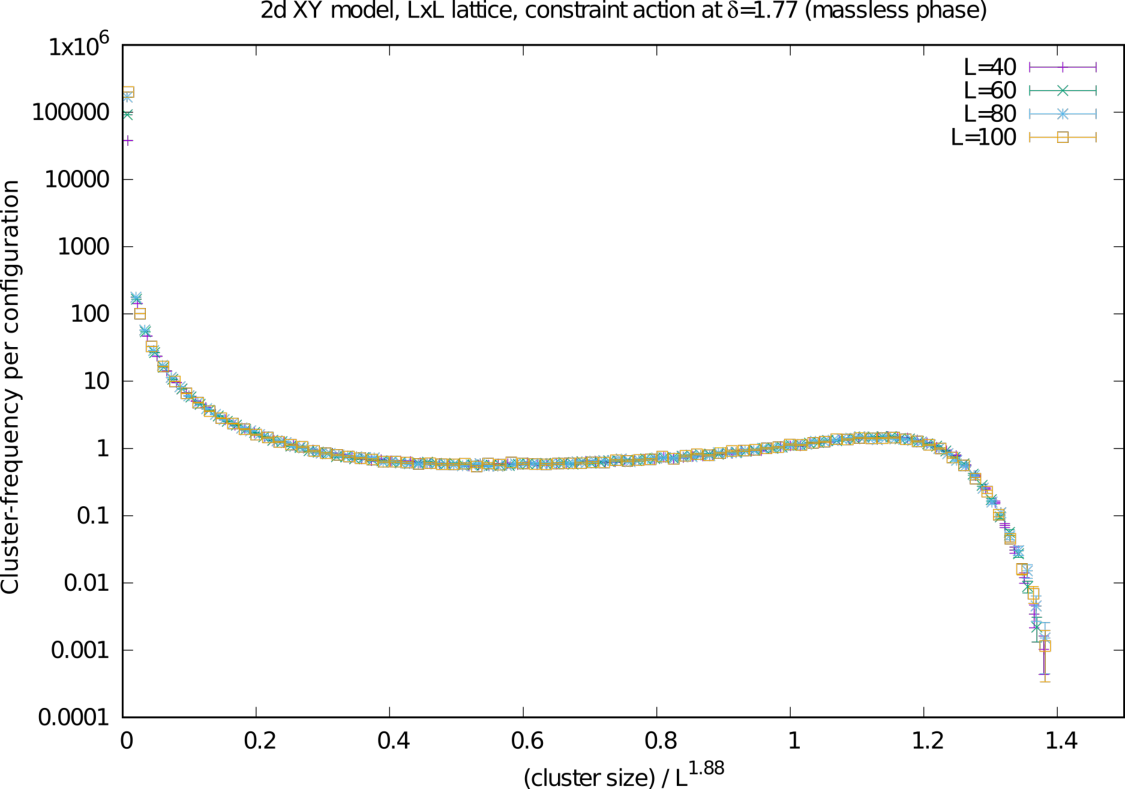
Next, we proceed to the massless phase, i.e. $\delta\leq\delta_{\rm c}\simeq 1.775$. Here each value of $\delta$, or each $1/g^{2}\geq 1/g_{\rm c}^{2}$ for the standard action, represents its own universality class. In a finite volume of size $L\times L$, $\xi$ is finite as well, and it turns out that — at fixed $\delta$ — the physical ratio $L/\xi$ is practically $L$-independent. This also holds for the second moment correlation length $\xi_{2}$ which is very close to $\xi$ but easier to measure ($\xi_{2}$ tends to be slightly shorter). For simplicity we are going to refer to $\xi_{2}$; its definition is reproduced e.g. in Ref. [5], Section 4. Fig. 4b refers to $\delta=1.77$ and $L=40,\dots,100$, where we consistently obtained $L/\xi_{2}\simeq 1.34$. Here the cluster-size is given in units of $L^{D}$, with the fractal dimension $D=1.88(1)$, which leads to precise cluster-size scaling (except for the few-site clusters).

When we repeat these simulations deeper in the massless phase, the ratio $L/\xi_{2}$ shrinks while $D$ gradually increases. For $\delta=1.775,1.7,1.6$, and $1.5$, we obtain $D=1.88(1),1.89(1),1.91(1)$, and $1.93(1)$, respectively. Ultimately, $D$ converges to $2$. Indeed, when $\delta$ approaches 0, all spins must be parallel and all bonds between nearest neighbors will be put with probability 1. As a result, at $\delta=0$ there is just one cluster which fills the entire space-time volume, and thus has dimension $D=2$.

The 3-d O(4) model can be interpreted as a high-temperature effective theory that captures the universal features of the finite temperature chiral phase transition of 2-flavor QCD in the chiral limit, provided that this transition is second order [23]. This is due to the equivalence of the symmetry breaking pattern ${\rm SU}(2)_{L}\times{\rm SU}(2)_{R}\to{\rm SU}(2)_{L=R}$ with ${\rm O}(4)\to{\rm O}(3)$. The 4-d O(4) model has topological Skyrmion excitations which may be interpreted as baryons [24]. At any fixed time, the total baryon number $B$ is given by the winding number in the homotopy group $\Pi_{3}(S^{3})=\mathbb{Z}$. The fermionic statistics and spin of the Skyrme-baryons are determined by the two elements of the homotopy group $\Pi_{4}(S^{3})=\mathbb{Z}(2)=\{\pm 1\}$, which represent the fermion sign in the corresponding functional integral. When the temperature is sufficiently high to imply dimensional reduction, Skyrmions become static and their sign problem associated with $\Pi_{4}(S^{3})$ disappears. Their topological baryon number, $B\in\Pi_{3}(S^{3})=\mathbb{Z}$, however, persists at high temperatures.

In this model, the meron concept, i.e. the assignment of well-defined half-integer topological baryon numbers to individual clusters, requires the restrictive constraint $\cos\delta>-1/3$ on the relative angles between neighboring spins within a simplex, such that only rather smooth configurations are admitted. It turns out that imposing this constraint restricts us to the low-temperature chirally broken phase. Since we are interested in the universal features of the chiral phase transition, we consider the standard action instead and study the cluster-size scaling for all clusters irrespective of their topological features. The critical inverse coupling was identified as $1/g_{\rm c}^{2}=0.93590(5)$ [25, 26].

A cluster-size scaling study is motivated at the critical point. Fig. 5a shows the matching of the histograms for $L^{3}$ lattices, where the cluster-size is successfully rescaled by $L^{D}$ with $D=2.485$.

It is interesting to ask whether the fractal dimension is related to the critical exponents of the chiral phase transition. Such a relation indeed exists for the $d$-dimensional Ising model. In that case, the magnetization $M=\sum_{\cal C}M_{\cal C}$ receives additive contributions from the individual Swendsen-Wang clusters [8]. All Ising spins inside a given cluster are parallel, so the absolute value of the magnetization of a cluster $|M_{\cal C}|$ is simply given by the cluster-size $|{\cal C}|$. Since the cluster magnetization changes sign under cluster flip, and since all clusters are independent, one obtains an improved estimator for the magnetic susceptibility

Hence, the cluster-size, whose distribution determines the fractal dimension, is directly related to $\chi_{\rm m}$. Using finite-size scaling of $\chi_{\rm m}$, for the Ising model one can analytically relate the fractal dimension to the critical exponents $\beta$ and $\nu$ [31, 32]

In the O($N$) models, all spins inside a Wolff-cluster are on the same side of the reflection hyperplane, but they are typically not parallel. As a result, the cluster-size is no longer directly related to $\chi_{\rm m}$ and thus the fractal dimension can no longer be analytically related to the critical exponents by the same argument. Remarkably, we find that the scaling law (6.2) also works in the 3-d O(4) model to high numerical accuracy. Ref. [26] reported (and we have independently confirmed) $\beta=0.380$ and $\nu=0.7377$, which implies $d-\beta/\nu=2.485$, in excellent agreement with our measurement of the fractal dimension $D$.

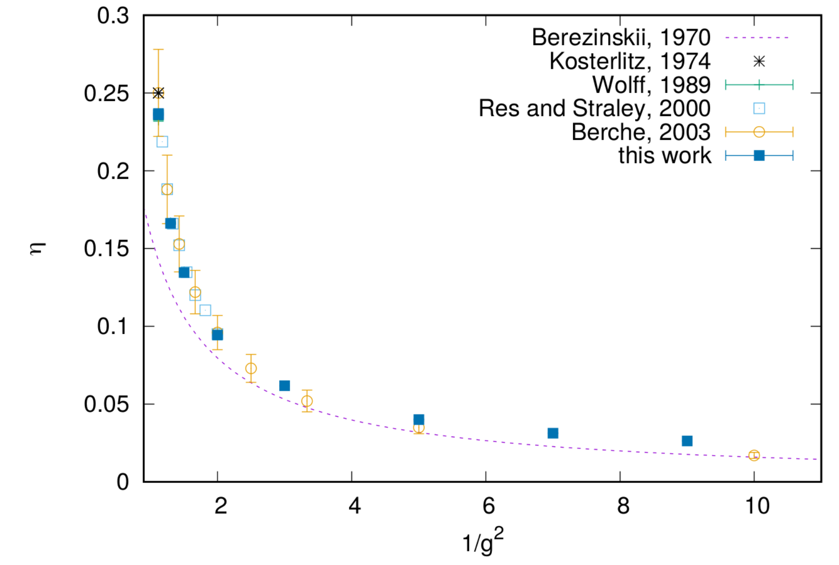
Encouraged by this result, we apply the scaling law (6.2) also to the 2-d O(2) model in the massless phase. It should be noted that, in that case, due to the exponentially diverging correlation length and susceptibility, $\beta$ and $\nu$, which characterize power-law divergences, are not defined. Based on hyperscaling, $2\beta/\nu$ is then replaced by the continuously varying critical exponent $\eta\leq\eta_{\rm c}=1/4$ [27], which characterizes the algebraic decay of spin correlations in the massless phase. Thus, $\eta$ determines the finite-size scaling of the susceptibility in the large-volume limit, $\chi_{\rm m}\propto L^{2-\eta}$. Replacing $\beta/\nu$ by $\eta/2$ in the scaling law (6.2), we obtain $D=2-\eta/2$. Fig. 5b shows $D$ as measured at various values of $1/g^{2}>1/g_{\rm c}^{2}$ in comparison with $d-\eta/2$. Indeed, the scaling law also holds in the 2-d O(2) model both at the BKT transition and inside the massless phase. The same has been observed using the topological action. At the BKT transition, $\eta$ approaches $\eta_{\rm c}=1/4$ which implies $D=1.875$, in agreement with the observed fractal dimension $D=1.88(1)$. In view of the scaling law, it would be interesting to also understand the value of the fractal dimension, again $D=1.88(1)$, that we obtained for the 2-d O(3) model.

Based on the cluster-size continuum scaling that we observed in a set of O($N$) models, we have argued that clusters can be interpreted as physical objects.

In the quantum mechanical 1-d O(2) model, the dimension $D$ of the clusters coincides with the dimension $d=1$. For $d$-dimensional quantum field theories with $d>1$, however, we observed a fractal dimension $D<d$. This implies that the physical clusters fill only a negligible fraction of space-time. In the continuum limit, space-time is filled with tiny few-site clusters, which do not display this scaling behavior. We also observed this in the broken phase of the 3-d O(4) model, where $D$ approaches $3$ as $1/g^{2}$ increases. In the Ising model the analytically derived scaling law (6.2) relates the fractal dimension $D$ to the critical exponents. We postulated the applicability of this scaling-law for general O($N$) models, and confirmed this numerically in the 2-d O(2) and 3-d O(4) model.

In the 2-d O(2) model, we identified semi-vortices and semi-anti-vortices that reside at the cluster boundaries in alternating order. Based on this, we introduced a criterion to decide whether a vortex and an anti-vortex form a bound pair. This holds the promise to provide deeper qualitative and quantitative insights into the mechanism of the BKT phase transition.

In models with a global topological charge, if an appropriate constraint on the relative angle between nearest-neighbor spins is implemented in the lattice action, we assigned a uniquely defined topological charge $Q_{\cal C}$ to each cluster. In particular, the merons (with $|Q_{\cal C}|=1/2$) are important carriers of topological charge. In the 1-d O(2) model, merons persist in the continuum limit, as we even showed analytically. In the 2-d O(3) model, on the other hand, the situation is more subtle. First of all, a power-law ultraviolet divergence of the topological susceptibility $\chi_{\rm t}$ due to dislocation lattice artifacts does not seem to arise. Instead, just like small instantons in a semi-classical investigation, meron-clusters of a small physical size give rise to a logarithmic divergence of $\chi_{\rm t}$. However, while the cluster-size distribution of all clusters collapses on a universal continuum curve, the size-distributions of the clusters with fixed topological charge $Q_{\cal C}$ do not converge in the continuum limit. In fact, multi-meron-clusters proliferate, diminish the probability of meron- and non-meron-clusters, and give rise to yet another logarithmic divergence of $\chi_{\rm t}$.

It would be most interesting to extend the stochastic definition of the physical topological charge carriers to other models, including 2-d $\mathbb{C}{\rm P}(N-1)$ models for $N>2$, the Schwinger model, as well as 4-d Yang-Mills theories, or QCD. In particular, if these objects could be tied directly to physical observables, via something like improved estimators, they could be established as relevant physical degrees of freedom with a solid field theoretical basis, beyond any semi-classical approximation. Unfortunately, for the models mentioned above, efficient cluster algorithms could not be constructed until now. In particular, Wolff-type embedding cluster algorithms are not efficient in $\mathbb{C}{\rm P}(N-1)$ models with $N>2$ [33, 34], and do not give rise to a meaningful definition of merons. Our study provides a strong motivation to keep searching for appropriate constructions, in order to deepen our understanding of the topological mechanisms that are responsible for the generation of a mass gap in non-linear $\sigma$-models and for confinement in gauge theories.

References

- [2] U. Wolff, Phys. Rev. Lett. 62 (1989) 361.
- [3] V. L. Berezinskiĭ, Zh. Eksp. Teor. Fiz. 59 (1970) 907 [Sov. Phys. JETP 32 (1971) 493]; Zh. Eksp. Teor. Fiz. 61 (1971) 1144 [Sov. Phys. JETP 34 (1972) 610].
- [4] J. M. Kosterlitz and D. J. Thouless, J. Phys. C 5 (1972) L124; J. Phys. C 6 (1973) 1181; J. Phys. C 7 (1974) 1046.
- [5] W. Bietenholz, U. Gerber, M. Pepe, and U.-J. Wiese, JHEP 1012 (2010) 020.
- [6] M. Bögli, F. Niedermayer, M. Pepe, and U.-J. Wiese, JHEP 1204 (2012) 117.
- [7] J. Balog, F. Niedermayer, M. Pepe, P. Weisz, and U.-J. Wiese, JHEP 1211 (2012) 140.
- [8] R. H. Swendsen and J.-S. Wang, Phys. Rev. Lett. 58 (1987) 86.
- [9] B. Berg and M. Lüscher, Nucl. Phys. B 190 (1981) 412.
- [10] W. Bietenholz, A. Pochinsky, and U.-J. Wiese, Phys. Rev. Lett. 75 (1995) 4524.
- [11] W. Bietenholz, R. Brower, S. Chandrasekharan, and U.-J. Wiese, Phys. Lett. B 407 (1997) 283.
- [12] T. Boyer, W. Bietenholz, and J. Wuilloud, Int. J. Mod. Phys. C 18 (2007) 1497.
- [13] S. Caspar, unpublished notes.
- [14] M. Lüscher, Nucl. Phys. B 200 (1982) 61.
- [15] M. Blatter, R. Burkhalter, P. Hasenfratz, and F. Niedermayer, Phys. Rev. D 53 (1996) 923.
- [16] W. Bietenholz, P. de Forcrand, U. Gerber, H. Mejía-Díaz, and I.O. Sandoval, Phys. Rev. D 98 (2018) 114501.
- [17] J. Balog and M. Niedermaier, Nucl. Phys. B 500 (1997) 421; Phys. Rev. Lett. 78 (1997) 4151.
- [18] W. Bietenholz, K. Cichy, P. de Forcrand, A. Dromard, and U. Gerber, PoS LATTICE2016 (2016) 321.
- [19] I. Horvath, S. J. Dong, T. Draper, F. X. Lee, K. F. Liu, N. Mathur, H. B. Thacker, and J. B. Zhang, Phys. Rev. D 68 (2003) 114505. E.-M. Ilgenfritz, K. Koller, Y. Koma, G. Schierholz, T. Streuer, and V. Weinberg, Phys. Rev. D 76 (2007) 034506.
- [20] M. Hasenbusch, J. Phys. A 38 (2005) 5869.
- [21] W. Bietenholz, M. Bögli, F. Niedermayer, M. Pepe, F. G. Rejón-Barrera, and U.-J. Wiese, JHEP 1303 (2013) 141.
- [22] W. Bietenholz, U. Gerber, and F. G. Rejón-Barrera, J. Stat. Mech. 1312 (2013) P12009.
- [23] K. Rajagopal and F. Wilczek, Nucl. Phys. B 399 (1993) 395.
- [24] T. H. R. Skyrme, Proc. Roy. Soc. Lond. A 260 (1961) 127; Nucl. Phys. B 31 (1962) 556.
- [25] M. Oevers, Diploma thesis, Bielefeld University, 1996.
- [26] J. Engels, L. Fromme, and M. Seniuch, Nucl. Phys. B 675 (2003) 533.
- [27] J. M. Kosterlitz, J. Phys. C 7 (1974) 1046.
- [28] U. Wolff, Nucl. Phys. B 322 (1989) 759.
- [29] I. Res and J. P. Straley, Phys. Rev. B 61 (2000) 14425.
- [30] B. Berche, J. Phys. A 36 (2003) 585.
- [31] D. Stauffer and A. Aharony, Introduction to Percolation Theory, Taylor & Francis, London, 1994.
- [32] W. Janke and A. M. J. Schakel, Phys. Rev. E 71 (2005) 036703.
- [33] K. Jansen and U.-J. Wiese, Nucl. Phys. B 370 (1992) 762.
- [34] S. Caracciolo, R. G. Edwards, A. Pelisetto, and A. D. Sokal, Nucl. Phys. B 403 (1993) 475.