A well aligned orbit for the 45 Myr old transiting Neptune DS Tuc AbJournal: ApJL
Abstract
DS Tuc Ab is a Neptune-sized planet that orbits around a G star in the 45 Myr old Tucana-Horologium moving group. Here, we report the measurement of the sky-projected angle between the stellar spin axis and the planet’s orbital axis, based on the observation of the Rossiter-McLaughlin effect during three separate planetary transits. The orbit appears to be well aligned with the equator of the host star, with a projected obliquity of . In addition to the distortions in the stellar absorption lines due to the transiting planet, we observed variations that we attribute to large starspots, with angular sizes of tens of degrees. The technique we have developed for simultaneous modeling of starspots and the planet-induced distortions may be useful in other observations of planets around active stars.
Keywords:
planetary systems — stars: individual (DS Tuc, TOI-200, TIC 410214984) techniques: spectroscopic, photometricI Introduction
Studying planets over a wide range of ages is the next best thing to being able to study planet formation and evolution in real time. The prospects for these types of studies have been greatly enhanced by recent discoveries of transiting planets around young stars. Data from the NASA K2 mission have been used to find planets in the 10-Myr-old Upper-Sco moving group (Mann et al. 2016b; David et al. 2016), the 20-Myr-old Taurus-Auriga group (David et al. 2019), and older clusters such as Praesepe and the Hyades (Mann et al. 2016a; Mann et al. 2017; Vanderburg et al. 2018; Rizzuto et al. 2018, e.g). These efforts have also resulted in the first determinations of the occurrence rates of close-in small planets in young associations and clusters, and allowed meaningful comparisons with the planet population around mature main-sequence field stars (Rizzuto et al. 2017).
DS Tuc Ab holds special importance amongst this population of planets. Discovered via observations with the Transiting Exoplanet Survey Satellite (Ricker et al. 2016, TESS, ), DS Tuc Ab is a planet residing in an 8-day period orbit around a member of the 45-Myr-old Tucana-Horologium moving group (Newton et al. 2019). What sets DS Tuc Ab apart from most of the previously discovered planets around young stars is the exceptional brightness of the host star . This enables a more in-depth characterization of the system, including the observations described here.
In this Letter, we present a determination of the sky-projected stellar obliquity of DS Tuc Ab based on ground-based optical spectroscopy spanning 3 transits. The obliquity angle is a tracer for any orbit-misaligning dynamical processes that the system might have undergone, assuming the initial condition exhibited good alignment. Dynamical interactions within stellar binary or planetary systems can determine the orbital plane inclination of close-in planets (Fabrycky & Tremaine 2007; Wu et al. 2007, e.g.). Protoplanetary disks may also become tilted due to the presence of stellar companions (Batygin 2012, e.g.). Reviews by Dawson & Johnson 2018 and Triaud 2018 summarize the set of mechanisms that can result in high obliquity planetary orbits, and the inferences made from the ensemble of obliquity measurements we have now amassed. Measuring the orbital obliquities of young planets is one pathway to understanding the processes that sculpt planetary systems. With these observations, as well as those reported independently by (Montet et al. 2019), DS Tuc Ab is now the youngest planetary system for which the stellar obliquity has been measured.
II Transit spectroscopic observations
The basis of the measurement technique is the Rossiter-McLaughlin effect, which utilizes changes in the profiles of the stellar absorption lines during a planetary transit. The changes in the stellar spectrum are sometimes analyzed as overall shifts in the central wavelengths of the lines. Young stars such as DS Tuc A present special challenges because they exhibit significant photometric and spectroscopic variability, due to large spots on their stellar surfaces. Here, we found it advantageous to analyze the distorted line profiles directly to best understand the stellar spots and their effect on our orbital obliquity measurement. Similarly, we also decided to observe three different transits for consistency checks in our obliquity derivations.
II.1 6.5 m Magellan – Planet Finder Spectrograph
We observed two transits with the Planet Finder Spectrograph (Crane et al. 2010, PFS,) on the 6.5 m Magellan Clay Telescope, located at Las Campanas Observatory, Chile. PFS is a high resolution echelle spectrograph, fed via a slit for our observations, yielding a spectral resolving power of over a spectral range of –. Typically, PFS is used for precise radial-velocity measurements and employs an iodine gas absorption cell for wavelength calibration. We did not use the iodine cell because we wanted to analyze the stellar absorption line profiles without the interference of the iodine spectrum.
The observations were conducted on 2019-08-19 and 2019-10-07 UTC. On the first night, we obtained 36 spectra starting at 03:20 and ending at 09:57 UTC. On the second night, we obtained 33 spectra in between 23:54 and 05:57 UTC. In both cases, the observations spanned the full transit. The integration time was 600 sec per spectrum. Wavelength solutions were determined with reference to spectra of the Thorium-Argon hallow cathode lamp, obtained at the beginning and the end of the night.
The stellar line profiles were derived from each spectrum via a least-squares deconvolution (LSD) over the wavelength range from 4000 to (Donati et al. 1997; Collier Cameron et al. 2010, following). A set of synthetic spectra from the ATLAS9 model atmospheres (Castelli & Kurucz 2004) were used as templates for the deconvolution. We constructed a master line profile based on an average of the ensemble of observations. The master line profile was then subtracted from each individual spectrum. The residuals display features due to both the planet and the starspots, and were analyzed further as described in Section III.
II.2 1.5 m SMARTS – CHIRON
We also observed a transit of DS Tuc Ab using the CHIRON facility (Tokovinin et al. 2013) on the 1.5 m Small and Moderate Aperture Research Telescope System (SMARTS) telescope, located at Cerro Tololo Inter-American Observatory (CTIO), Chile. CHIRON is a high resolution echelle spectrograph fed from an image slicer through a fiber bundle, with a spectral resolving power of over the wavelength region from 4100 to Å. A total of 21 CHIRON spectra were obtained during the 2019-08-11 transit of DS Tuc Ab, from 02:26 to 05:52 UTC, with 600 sec of integration per exposure. This covered the full duration of the transit. Line profiles were derived from the CHIRON spectra via the same LSD analysis described in Section II.1.
Stellar atmospheric parameters, including effective temperature, surface gravity, and metallicity, were also measured from the CHIRON observations. These parameters were measured by matching the CHIRON spectra against an interpolated library of observed spectra classified by the Spectral Classification Pipeline (Buchhave et al. 2012). We find DS Tuc A to have an effective temperature of K, surface gravity of , and metallicity of .
III Analysis and Modeling
As mentioned above, modeling the spectroscopic transits of DS Tuc Ab presents an interesting challenge. The TESS light curve shows spot-induced photometric variability on the order of 2%, which is ten times larger than the amplitude of the transit signals. We found it necessary to fit each residual spectrum with a model that includes the influence of star spots and the Rossiter-McLaughlin effect.
The spots are modeled as circular patches on the stellar photosphere, each with a uniform surface brightness which is darker than the surrounding photosphere. Each spot is parameterized by its angular radius on the photosphere (), latitude (), and initial longitude (). The longitudes are defined such that corresponds to a distortion at the blue extreme of the spectral line. This is similar to the parameterization of the spot modeling adopted by Boisse et al. 2012, though we adopt to use a simple grid numerical integration over the spots to compute their effects on the stellar line profile. For simplicity, we assumed the stellar rotation axis is perpendicular to the line of sight, i.e., we forfeited any attempt to constrain the stellar inclination angle from the data. This is because such determinations generally yield degenerate posteriors, and because the assumption is compatible with the combination of the best estimate for the projected stellar rotation velocity (), the photometric rotation period (2.85 days), and the stellar radius () (Newton et al. 2019).
The darkening effect of each spot was calculated via a numerical integration over the stellar surface, accounting for limb darkening, instrumental broadening, and radial-tangential macroturbulence (Gray 2005). Another key parameter in the model is the number of spots. We used the Bayesian Information Criterion to decide on the best number of spots needed to fit each transit sequence. For the 2019-08-11 CHIRON transit, we did not include any spots in the model. For the 2019-08-19 and 2019-10-07 PFS transits, we used four spots. The Appendix details the Bayesian information criterion and the best fit value for each trialed spot configuration in our analyses. Figure 1 illustrates the spot model for the 2019-10-07 transit (an animated version of both transits are available in the online edition). We note that the TESS light curves show significant spot evolution over its observation period of days. As such we do not expect the spot configuration from our two PFS observations to be related.
We note that these are idealistic models that likely do not capture the true complexity of the stellar surface. In particular, whilst the 2019-08-11 CHIRON transit requires no spot corrections, this is only because the average line profile subtracts well from each individual exposure given the short time baseline of the observation. Spectroscopic observations encompassing the full rotational phase coverage are required to reconstruct realistic representations of the spot coverage for DS Tuc A, as shown by classical Doppler imaging exercises (Donati et al. 1997, e.g.).

We took a comprehensive approach to determining the system parameters, by performing a simultaneous global modeling with:
- 1.
The PFS and CHIRON spectra spanning 3 transits,
- 2.
The TESS transit light curve,
- 3.
The Spitzer transit light curves from Newton et al. 2019,
- 4.
The spectroscopically derived stellar effective temperature and photometric spectral energy distribution available in literature,
- 5.
The trigonometric parallax reported in Gaia Data Release 2 (Gaia Collaboration et al. 2018),
- 6.
The MIST theoretical stellar-evolutionary models (Dotter 2016; Choi et al. 2016), and
- 7.
The estimated age of the Tucana-Horologium moving group.
Our overall approach was similar to the one described by Zhou et al. 2019. We incorporate free parameters for the transit centroid timing , period , planet-star radius ratio , line of sight inclination , projected obliquity , stellar mass and radius , parallax, rotational broadening , macroturbulent broadening , as well as the parameters describing each star spot described previously. Parallax and are constrained by Gaussian priors about the Gaia and spectroscopically measured values. The stellar effective temperature is also constrained by a Gaussian prior about our spectroscopic value. We fix the stellar metallicity to Solar to be consistent with the analysis in the discovery paper (Newton et al. 2019). The age of the star is constrained by a Gaussian prior of Myr, based on the age of the Tucana-Horologium moving group (Kraus et al. 2014; Bell et al. 2015). Uniform priors are applied to the remaining parameters. The light curves were modeled as per Mandel & Agol 2002. We assume no local reddening affecting the spectral energy distribution of DS Tuc Ab. The local maximum reddening in the region around DS Tuc A is from dust maps by Schlafly & Finkbeiner 2011, and has minimal impact to our analysis. The line profile variation induced by the planet (its “Doppler shadow”) was modeled by performing the two-dimensional integral over the area of the star covered by the planet, incorporating local radial-tangential macroturbulence, limb darkening, and the instrument broadening. The planet’s orbit was assumed to be circular.
To determine the best-fitting parameters and the associated uncertainties, we used the Markov Chain Monte Carlo method as implemented in the emcee software package (Foreman-Mackey et al. 2013). Table 1 gives the results. We also tried re-fitting the data using the same procedure but including only the data from one of the spectroscopic transits, rather than fitting all 3 datasets together. We verified that the results were consistent, regardless of which spectroscopic transit was chosen.
Figure 2 depicts the analysis of the PFS spectroscopic data observation in stages. Shown are the time series of the line profile variations, the residuals after subtracting the model for the effects of spots, the model for the effect of the planet, and the residuals after subtracting all the components of the best-fitting model. The planetary perturbation travels the full extent of the spectral line, from the blue side to the red side, implying that the orbital and rotational motion are well-aligned. Figure 3 (top panels) shows all 3 spectroscopic datasets after subtracting the best-fitting spot model, thereby isolating the planetary signal. The signals are all consistent with one another.
In addition, our spot model can be used to reconstruct a spot-modulated light curve of DS Tuc A. The amplitude of the model rotation curve is 10% for 2019-08-10, and 3% for 2019-10-07. In comparison the amplitude of the TESS light curve spot modulation is at the 2% level, with significant variations in the modulation amplitude through the course of the TESS observations.
PFS 2019-08-11

PFS 2019-10-07


| Parameter | Joint model | CHIRON 2019-08-11 | PFS 2019-08-19 | PFS 2019-10-07 |
|---|---|---|---|---|
| Light curve parameters | ||||
| (days) . | ||||
| () . | ||||
| . | ||||
| . | ||||
| (deg) . | ||||
| Stellar parameters | ||||
| () . | ||||
| () . | ||||
| Age (Myr) . | ||||
| () . | ||||
| () . | ||||
| Linear limb darkening coefficient . | 0.358 (fixed) | |||
| Quadratic limb darkening coefficient . | 0.249 (fixed) | |||
| Linear limb darkening coefficient . | 0.0697 (fixed) | |||
| Quadratic limb darkening coefficient . | 0.1416 (fixed) | |||
| Star Spot parameters | ||||
| 2019-08-19 Spot 1 Contrast . | ||||
| 2019-08-19 (deg) Spot 1 Radius . | ||||
| 2019-08-19 (deg) Spot 1 Initial Phase . | ||||
| 2019-08-19 (deg) Spot 1 Latitude . | ||||
| 2019-08-19 Spot 2 Contrast . | ||||
| 2019-08-19 (deg) Spot 2 Radius . | ||||
| 2019-08-19 (deg) Spot 2 Initial Phase . | ||||
| 2019-08-19 (deg) Spot 2 Latitude . | ||||
| 2019-08-19 Spot 3 Contrast . | ||||
| 2019-08-19 (deg) Spot 3 Radius . | ||||
| 2019-08-19 (deg) Spot 3 Initial Phase . | ||||
| 2019-08-19 (deg) Spot 3 Latitude . | ||||
| 2019-08-19 Spot 4 Contrast . | ||||
| 2019-08-19 (deg) Spot 4 Radius . | ||||
| 2019-08-19 (deg) Spot 4 Initial Phase . | ||||
| 2019-08-19 (deg) Spot 4 Latitude . | ||||
| 2019-10-07 Spot 1 Contrast . | ||||
| 2019-10-07 (deg) Spot 1 Radius . | ||||
| 2019-10-07 (deg) Spot 1 Initial Phase . | ||||
| 2019-10-07 (deg) Spot 1 Latitude . | ||||
| 2019-10-07 Spot 2 Contrast . | ||||
| 2019-10-07 (deg) Spot 2 Radius . | ||||
| 2019-10-07 (deg) Spot 2 Initial Phase . | ||||
| 2019-10-07 (deg) Spot 2 Latitude . | ||||
| 2019-10-07 Spot 3 Contrast . | ||||
| 2019-10-07 (deg) Spot 3 Radius . | ||||
| 2019-10-07 (deg) Spot 3 Initial Phase . | ||||
| 2019-10-07 (deg) Spot 3 Latitude . | ||||
| 2019-10-07 Spot 4 Contrast . | ||||
| 2019-10-07 (deg) Spot 4 Radius . | ||||
| 2019-10-07 (deg) Spot 4 Initial Phase . | ||||
| 2019-10-07 (deg) Spot 4 Latitude . | ||||
| Planetary parameters | ||||
| () . | ||||
| (deg) . | ||||
| (AU) . | ||||
III.1 The Rossiter-McLaughlin effect
It is also possible to visualize the results by computing the apparent radial velocity shift of the entire line profile induced by all the line profile distortions. Figure 3 (bottom panel) shows these “anomalous radial velocities” based on all 3 transit observations. Before making this plot, long-term trends in the PFS radial velocities were removed by subtracting the best-fitting quadratic function of time to the out-of-transit data. This trend need not be astrophysical; because the observations were obtained without the use of an iodine gas absorption cell, the radial velocities are susceptible to intra-night drift of the instrumental profile and wavelength solution. We computed a model for the anomalous radial velocity based on the system parameters in Table 1, using code provided by Boué et al. 2013. The model agrees well with the data, even without any further tuning of the model parameters. With this way of displaying and analyzing the data, the effects of spots are not as obvious. This is because the spots migrate smoothly across a significant part of the stellar surface over the time scale of the transit.
We note, though, that not accounting for the influence of spots can cause a systematic bias in the resulting derived obliquities from the Rossiter-McLaughlin effect. If one part of the star is dimmer due to the presence of a group of spots, then the overall weighted velocity variation induced by a planet with be affected by the specific part of the star the planet transits through. This bias is irrespective of any possible spot-crossing events. Systematic uncertainties arising from such issues will need to be accounted in the error budget in Rossiter-McLaughlin observations (Oshagh et al. 2018, e.g.). A light curve motivated spot-modeling exercise, in conjunction with an Rossiter-McLaughlin observation, can encompass such systematic uncertainties (Montet et al. 2019).
IV Discussion
The finding of a well-aligned star and planetary orbit would not have been surprising a decade ago. Since then, though, we have learned that stellar obliquities are sometimes very large (Winn et al. 2010a; Albrecht et al. 2012, e.g.), and no longer take spin-orbit alignment for granted. High obliquity orbits have been interpreted as evidence for dynamical processes that tilt the orbit of a giant planet after its formation within the gaseous protoplanetary disk. The large majority of previous obliquity measurements have been made for close-in giant planets around mature-age stars (Figure 4).
DS Tuc A stands out from previous systems not only because of its age. With a radius of 6 , the planet is more representative of the abundant population of close-orbiting planets that were revealed clearly by the NASA Kepler mission (Dong & Zhu 2013; Zhu et al. 2018, see, e.g.,), and have stimulated many new ideas about planet formation and orbital evolution. Of these systems hosting small planets, few have had their orbital obliquities measured. Of those with spectroscopic, spot-crossing, or astro-seismic constraints on orbital obliquities, single-planet close-in Neptune systems can often be found in misaligned orbits, such as HAT-P-11b (Winn et al. 2010b; Hirano et al. 2011; Sanchis-Ojeda & Winn 2011), Kepler-63b (Sanchis-Ojeda et al. 2013), WASP-107b (Dai & Winn 2017), GJ436b (Bourrier et al. 2018), and Kepler-408b (Kamiaka et al. 2019). Longer period Neptunes found in multi-planet systems, such as Kepler-25 (Albrecht et al. 2013; Benomar et al. 2014; Campante et al. 2016), Kepler-65 (Chaplin et al. 2013), and HD 106315 (Zhou et al. 2018) have been found in well aligned orbits. Misaligned multiplanet Neptune systems do exist around main-sequence stars though (Dalal et al. 2019, HD 3167,), and an extended sample of youthful planetary systems will help identify the mechanisms responsible for such systems.
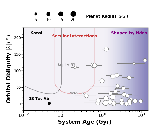
DS Tuc Ab has similar attributes to many in the lone hot Neptune population. It lies in a close-in 8-day period orbit, and has no additional transiting companions detected. The radius of DS Tuc Ab is expected to shrink continuously as it undergoes cooling, and is likely to be of at ages Gyr (Howe & Burrows 2015, e.g.). A number of mechanisms can be ruled out in influencing the dynamical history of the system. DS Tuc is a hierarchical triple system, with the transiting Neptune orbiting DS Tuc A, and the binary companion DS Tuc B orbiting A at a median separation of AU, in an orbit about DS Tuc A that is likely co-planar with the orbit of the planet (Newton et al. 2019). In systems with inclined exterior companions, fast Kozai interactions (Wu et al. 2007, e.g.) can be responsible in producing the population of close-in hot Jupiters within timescales of to years in hierarchical triple systems. The likely co-planar orbit of DS Tuc B with A makes Kozai interactions unlikely the cause of DS Tuc Ab’s close-in orbit. Secular planet-planet interactions may account for a portion of the close-in Neptune population. These interactions take place over timescales of hundreds of millions of years (Wu & Lithwick 2011), resulting in a uniform distribution of orbital obliquities. The young age and lack of an inclined orbit suggests that DS Tuc Ab is not an example of secular planet-planet interactions. Similarly, Yee et al. 2018 attributed the polar orbit of HAT-P-11b to nodal precession induced by an inclined, eccentric, non-transiting outer planet. Such precession can occur on fast timescales ( Myr for HAT-P-11b). Long-term radial velocity or astrometric monitoring of DS Tuc A may help reveal additional non-transiting planetary companions in the system, but the low orbital obliquity we measure may already help rule out inclined planetary perturbers. Spin-orbit misalignment via tilting of the protoplanetary disk may occur in some binaries at time scales of Myr, but such excitation of the disk spin-orbit angle also requires an inclined stellar companion (Batygin 2012, e.g.). Zhan et al. 2019 suggest that some single stars may also have inner disks tilted with respect to the stellar spin axis. The probable well aligned binary orbit of DS Tuc B and the low obliquity of DS Tuc Ab is consistent with the lack of any large disk inclination early in its formation history.
With an extensive set of mechanisms that can influence the evolution of close-in planets, establishing the obliquity distribution for young planets is one avenue that can help disentangle the histories of these planetary systems. Establishing this distribution requires the efforts of all-sky surveys like the new discoveries from the TESS mission.
References
- Akeson et al. (2013) Akeson, R. L., Chen, X., Ciardi, D., et al. 2013, PASP, 125, 989
- Albrecht et al. (2013) Albrecht, S., Winn, J. N., Marcy, G. W., et al. 2013, ApJ, 771, 11
- Albrecht et al. (2012) Albrecht, S., Winn, J. N., Johnson, J. A., et al. 2012, ApJ, 757, 18
- Batygin (2012) Batygin, K. 2012, Nature, 491, 418
- Bell et al. (2015) Bell, C. P. M., Mamajek, E. E., & Naylor, T. 2015, MNRAS, 454, 593
- Benomar et al. (2014) Benomar, O., Masuda, K., Shibahashi, H., & Suto, Y. 2014, PASJ, 66, 94
- Boisse et al. (2012) Boisse, I., Bonfils, X., & Santos, N. C. 2012, A&A, 545, A109
- Boué et al. (2013) Boué, G., Montalto, M., Boisse, I., Oshagh, M., & Santos, N. C. 2013, A&A, 550, A53
- Bourrier et al. (2018) Bourrier, V., Lovis, C., Beust, H., et al. 2018, Nature, 553, 477
- Buchhave et al. (2012) Buchhave, L. A., Latham, D. W., Johansen, A., et al. 2012, Nature, 486, 375
- Campante et al. (2016) Campante, T. L., Lund, M. N., Kuszlewicz, J. S., et al. 2016, ApJ, 819, 85
- Castelli & Kurucz (2004) Castelli, F., & Kurucz, R. L. 2004, ArXiv Astrophysics e-prints, astro-ph/0405087
- Chaplin et al. (2013) Chaplin, W. J., Sanchis-Ojeda, R., Campante, T. L., et al. 2013, ApJ, 766, 101
- Choi et al. (2016) Choi, J., Dotter, A., Conroy, C., et al. 2016, ApJ, 823, 102
- Collier Cameron et al. (2010) Collier Cameron, A., Guenther, E., Smalley, B., et al. 2010, MNRAS, 407, 507
- Crane et al. (2010) Crane, J. D., Shectman, S. A., Butler, R. P., et al. 2010, in Society of Photo-Optical Instrumentation Engineers (SPIE) Conference Series, Vol. 7735, Proc. SPIE, 773553
- Dai & Winn (2017) Dai, F., & Winn, J. N. 2017, AJ, 153, 205
- Dalal et al. (2019) Dalal, S., Hébrard, G., Lecavelier des Étangs, A., et al. 2019, A&A, 631, A28
- David et al. (2016) David, T. J., Hillenbrand, L. A., Petigura, E. A., et al. 2016, Nature, 534, 658
- David et al. (2019) David, T. J., Cody, A. M., Hedges, C. L., et al. 2019, AJ, 158, 79
- Dawson & Johnson (2018) Dawson, R. I., & Johnson, J. A. 2018, ARA&A, 56, 175
- Donati et al. (1997) Donati, J.-F., Semel, M., Carter, B. D., Rees, D. E., & Collier Cameron, A. 1997, MNRAS, 291, 658
- Dong & Zhu (2013) Dong, S., & Zhu, Z. 2013, ApJ, 778, 53
- Dotter (2016) Dotter, A. 2016, ApJS, 222, 8
- Fabrycky & Tremaine (2007) Fabrycky, D., & Tremaine, S. 2007, ApJ, 669, 1298
- Foreman-Mackey et al. (2013) Foreman-Mackey, D., Hogg, D. W., Lang, D., & Goodman, J. 2013, PASP, 125, 306
- Gaia Collaboration et al. (2018) Gaia Collaboration, Brown, A. G. A., Vallenari, A., et al. 2018, A&A, 616, A1
- Gray (2005) Gray, D. F. 2005, The Observation and Analysis of Stellar Photospheres
- Hirano et al. (2011) Hirano, T., Narita, N., Shporer, A., et al. 2011, PASJ, 63, 531
- Howe & Burrows (2015) Howe, A. R., & Burrows, A. 2015, ApJ, 808, 150
- Kamiaka et al. (2019) Kamiaka, S., Benomar, O., Suto, Y., et al. 2019, AJ, 157, 137
- Kraus et al. (2014) Kraus, A. L., Shkolnik, E. L., Allers, K. N., & Liu, M. C. 2014, AJ, 147, 146
- Mandel & Agol (2002) Mandel, K., & Agol, E. 2002, ApJ, 580, L171
- Mann et al. (2016a) Mann, A. W., Gaidos, E., Mace, G. N., et al. 2016a, ApJ, 818, 46
- Mann et al. (2016b) Mann, A. W., Newton, E. R., Rizzuto, A. C., et al. 2016b, AJ, 152, 61
- Mann et al. (2017) Mann, A. W., Gaidos, E., Vanderburg, A., et al. 2017, AJ, 153, 64
- Montet et al. (2019) Montet, B. T., Feinstein, A. D., Luger, R., et al. 2019, arXiv e-prints, arXiv:1912.03794
- Newton et al. (2019) Newton, E. R., Mann, A. W., Tofflemire, B. M., et al. 2019, ApJ, 880, L17
- Oshagh et al. (2018) Oshagh, M., Triaud, A. H. M. J., Burdanov, A., et al. 2018, A&A, 619, A150
- Ricker et al. (2016) Ricker, G. R., Vanderspek, R., Winn, J., et al. 2016, in Proc. SPIE, Vol. 9904, Space Telescopes and Instrumentation 2016: Optical, Infrared, and Millimeter Wave, 99042B
- Rizzuto et al. (2017) Rizzuto, A. C., Mann, A. W., Vanderburg, A., Kraus, A. L., & Covey, K. R. 2017, AJ, 154, 224
- Rizzuto et al. (2018) Rizzuto, A. C., Vanderburg, A., Mann, A. W., et al. 2018, AJ, 156, 195
- Sanchis-Ojeda & Winn (2011) Sanchis-Ojeda, R., & Winn, J. N. 2011, ApJ, 743, 61
- Sanchis-Ojeda et al. (2013) Sanchis-Ojeda, R., Winn, J. N., Marcy, G. W., et al. 2013, ApJ, 775, 54
- Schlafly & Finkbeiner (2011) Schlafly, E. F., & Finkbeiner, D. P. 2011, ApJ, 737, 103
- Tokovinin et al. (2013) Tokovinin, A., Fischer, D. A., Bonati, M., et al. 2013, PASP, 125, 1336
- Triaud (2018) Triaud, A. H. M. J. 2018, The Rossiter-McLaughlin Effect in Exoplanet Research, 2
- Vanderburg et al. (2018) Vanderburg, A., Mann, A. W., Rizzuto, A., et al. 2018, AJ, 156, 46
- Winn et al. (2010a) Winn, J. N., Fabrycky, D., Albrecht, S., & Johnson, J. A. 2010a, ApJ, 718, L145
- Winn et al. (2010b) Winn, J. N., Johnson, J. A., Howard, A. W., et al. 2010b, ApJ, 723, L223
- Wu & Lithwick (2011) Wu, Y., & Lithwick, Y. 2011, ApJ, 735, 109
- Wu et al. (2007) Wu, Y., Murray, N. W., & Ramsahai, J. M. 2007, ApJ, 670, 820
- Yee et al. (2018) Yee, S. W., Petigura, E. A., Fulton, B. J., et al. 2018, AJ, 155, 255
- Zhan et al. (2019) Zhan, Z., Günther, M. N., Rappaport, S., et al. 2019, ApJ, 876, 127
- Zhou et al. (2018) Zhou, G., Rodriguez, J. E., Vanderburg, A., et al. 2018, AJ, 156, 93
- Zhou et al. (2019) Zhou, G., Bakos, G. Á., Bayliss, D., et al. 2019, AJ, 157, 31
- Zhu et al. (2018) Zhu, W., Petrovich, C., Wu, Y., Dong, S., & Xie, J. 2018, ApJ, 860, 101
To determine the number of spots required to best model our spectroscopic transit observations, we attempted fits of individual observations with a varying number of spots. The BIC and resulting projected obliquity values of each fit are presented in Table 2.
| 2019-08-11 CHIRON | 2019-08-19 PFS | 2019-10-07 PFS | ||||
|---|---|---|---|---|---|---|
| No. of Spots | BIC | Projected Obliquity | BIC | Projected Obliquity | BIC | Projected Obliquity |
| 0 | 4880 | 4.24 | 3750 | 3.20 | 6566 | 0.45 |
| 1 | 5845 | 4.70 | 2454 | -0.76 | 5182 | -2.57 |
| 2 | 5836 | 0.31 | 1980 | 3.77 | 2163 | 0.47 |
| 3 | 5898 | 0.89 | 1852 | 3.56 | 1872 | 2.35 |
| 4 | 5917 | 2.88 | 1647 | 3.15 | 1811 | 2.54 |
| 5 | 1942 | 3.77 | 2027 | 0.72 | ||
| 6 | 1724 | 3.38 | 1961 | 4.23 | ||