Contrast Trees and Distribution Boosting
Abstract
A new method for decision tree induction is presented. Given a set of predictor variables and two outcome variables and associated with each , the goal is to identify those values of for which the respective distributions of and , or selected properties of those distributions such as means or quantiles, are most different. Contrast trees provide a lack-of-fit measure for statistical models of such statistics, or for the complete conditional distribution , as a function of . They are easily interpreted and can be used as diagnostic tools to reveal and then understand the inaccuracies of models produced by any learning method. A corresponding contrast boosting strategy is described for remedying any uncovered errors thereby producing potentially more accurate predictions. This leads to a distribution boosting strategy for directly estimating the full conditional distribution of at each under no assumptions concerning its shape, form or parametric representation.
Keywords: prediction diagnostics, classification, regression, boosting, quantile regression, conditional distribution estimation
1 Introduction
In statistical (machine) learning one has a system under study with associated attributes or variables. The goal is to estimate the unknown value of one of the variables , given the known joint values of other (predictor) variables associated with the system. It is seldom the case that a particular set of –values gives rise to a unique value for . There are quantities other than those in that influence whose values are neither controlled nor observed. Specifying a particular set of joint values for results in a probability distribution of possible -values, , induced by the varying values of the uncontrolled quantities. Given a sample of previous solved cases, the goal is to estimate the distribution , or some of its properties, as a function of the predictor variables . These can then be used to predict likely values of realized at each .
Usually only a single property of is used for prediction, namely a measure of its central tendency such as the mean or median. This provides no information concerning individual accuracy of each prediction. Only average accuracy over a set of predictions (cross-validation) can be determined. In order to estimate individual prediction accuracy at each one needs additional properties of such as various quantiles, or the distribution itself. These can be estimated as functions of using maximum likelihood or minimum risk techniques. Such methods however do not provide a measure of accuracy (goodness-of-fit) for their respective estimates as functions of . There is no way to know how well the results actually characterize the distribution of at each .
Contrast trees can be used to assess lack-of-fit of any estimate of , or its properties (mean, quantiles), as a function of . In cases where the fit is found to be lacking, contrast boosting applied to the output can often improve accuracy. A special case of contrast boosting, distribution boosting, can be used to estimate the full conditional distribution under no assumptions. Contrast trees can also be used to uncover concept drift and reveal discrepancies in the predictions of different learning algorithms.
2 Contrast trees
A classification or regression tree partitions the space of - values into easily interpretable regions defined by simple conjunctive rules. The goal is to produce regions in - space such that the variation of values within each is made small. A contrast tree also partitions the - space into similarly defined regions, but with a different purpose. There are two outcome variables and associated with each . The goal is to find regions in - space where the values of the two variables are most different.
In some applications of contrast trees the outcomes and can be different functions of , and , such as predictions produced by two different learning algorithms. The goal of the contrast tree is then to identify regions in - space where the two predictions most differ. In other cases the outcome may be observations of a random variable assumed to be drawn from some distribution at , . The quantity might be an estimate for some property of that distribution such as its estimated mean or -th quantile as a function of . One would like to identify - values where the estimates appear to be the least accurate. Alternatively itself could be a random variable independent of (given ) with distribution and interest is in identifying regions of - space where the two distributions and most differ.
In these applications contrast trees can be used as diagnostics to ascertain the lack-of-fit of statistical models to data or to other models. As with other tree based methods the uncovered regions are defined by conjunctive rules based on simple logical statements concerning the variable values. Thus it is straightforward to understand the joint predictor variable values at which discrepancies have been identified. Such information may temper confidence in some predictions or suggest ways to improve accuracy.
In prediction problems is taken to be an estimate of some property of the distribution , or of the distribution itself. One way to improve accuracy is to modify the predicted values in a way that reduces their discrepancy with the actual values as represented by the data. Contrast trees attempt to identify regions of - space with the largest discrepancies. The - values within in each such region can then be modified to reduce discrepancy with . This produces new values of which can then be contrasted with using another contrast tree. This process can then be applied to the regions of the new tree thereby producing further modified - values. This “boosting” strategy of successively building contrast trees on the output of previously induced trees can be continued until the average discrepancy stops improving.
3 Building contrast trees
The data consists of observations each with a joint set of predictor variable values and two outcome variables and . Contrast trees are constructed from this data in an iterative manner. At the th iteration the tree partitions the space of - values into disjoint regions each containing a subset of the data . At the first iteration there is a single region containing the entire data set. Associated with any data subset is a discrepancy measure between the and values of the subset
| (1) |
Choice of a particular discrepancy measure depends on the specific application as discussed in Section 4.
At the next ()st iteration each of the regions defined at the th iteration () are provisionally partitioned (split) into two regions and ( ). Each of these “daughter” regions contains its own data subset with associated discrepancy measure and (1). The quality of the split is defined as
| (2) |
where and are the fraction of observations in the “parent” region associated with each of the two daughters.
The types of splits considered here are the same as in ordinary classification and regression trees (Breiman et al 1984). Each involves one of the predictor variables . For numeric variables splits are specified by a particular value of that variable (split point) . The corresponding daughter regions are defined by
| (3) | ||||
For categorical variables (factors) the respective levels are ordered by discrepancy (1). The discrepancy at each respective level of the factor for the observations in the th region is computed. Splits are then considered in this order.
Split quality (2) is evaluated jointly for all current regions , all predictor variables, and all possible splits of each variable. The region with largest estimated split improvement
| (4) |
is then chosen to create two new regions (3). Here (1) is the discrepancy associated with the data in the parent region and are corresponding discrepancies of the data subsets in the two daughters. These two new regions replace the corresponding parent producing total regions. Splitting stops when no estimated improvement (4) is greater than zero, the tree reaches a specified size or the observation count within all regions is below a specified threshold.
4 Discrepancy measures
By defining different discrepancy measures contrast trees can be applied to a variety of different problems. Even within a particular type of problem there may be a number of different appropriate discrepancy measures that can be used.
When the two outcomes are simply functions of , and , any quantity that reflects their difference in values at the same can be used to form a discrepancy measure such as
If is a random variable and is an estimate for a property of its conditional distribution at , , such as its mean or th quantile , a natural discrepancy measure is
| (5) |
Here is the value of the corresponding statistic computed for observations in the region and is an appropriate measure of central tendency for the corresponding estimates.
If both and are both independent random variables associated with each , a discrepancy measure reflects the distance between their respective distributions. There are many proposed empirical measures of distribution distance. Every two–sample test has one. For the examples below a variant of the Anderson–Darling (Anderson and Darling 1954) statistic is used. Let represent the pooled sample in a region . Then discrepancy between the distributions of and is taken to be
| (6) |
where is the th value of is sorted order, and and are the respective empirical cumulative distributions of and . Note that this discrepancy measure (6) can be employed in the presence of arbitrarily censored or truncated data simply by employing a nonparametric method to estimate the respective CDF’s such as Turnbul (1976) .
Discrepancy measures are often customized to particular individual applications. In this sense they are similar to loss criteria in prediction problems. However, in the context of contrast trees (and boosting) there is no requirement that they be convex or even differentiable. Several such examples are provided in the Appendix.
5 Boosting contrast trees
As indicated above, and illustrated in the examples presented below and in the Appendix, contrast trees can be employed as diagnostics to examine the lack of accuracy of predictive models. To the extent that inaccuracies are uncovered, boosted contrast trees can be used to attempt to mitigate them, thereby producing more accurate predictions. Contrast boosting derives successive modifications to an initially specified , each reducing its discrepancy with over the data. Prediction then involves starting with the initial value of and then applying the modifications to produce the resulting estimate.
5.1 Estimation contrast boosting
In this case is taken to be an estimate of some parameter of . The - values within each region of a contrast tree can be modified so that the discrepancy (1) with is zero in that region
| (7) |
This in turn yields zero average discrepancy between and over the regions defined by the terminal nodes of the corresponding contrast tree. However, there may well be other partitions of the - space defining different regions for which this discrepancy is not small. These may be uncovered by building a second tree to contrast with producing updates
| (8) |
These in turn can be contrasted with to produce new regions and corresponding updates . Such iterations can be continued times until the updates become small. As with gradient boosting (Friedman 2001) performance accuracy is often improved by imposing a learning rate. At each step the computed update in each region is reduced by a factor . That is, in (8).
Each tree in the boosted sequence partitions the - space into a set of regions . Any point lies within one region of each tree with corresponding update . Starting with a specified initial value the estimate at is then
| (9) |
5.2 Distribution contrast boosting
Here and are both considered to be random variables independently generated from respective distributions and . The purpose of a contrast tree is to identify regions of - space where the two distributions most differ. The goal of distribution boosting is to estimate a (different) transformation of at each , , such that the distribution of the transformed variable is the same as that of at . That is,
| (10) |
Thus, starting with values sampled from a known distribution at each , one can use the estimated transformation to obtain an estimate of the - distribution at that . Note that the transformation is usually a different function of at each different .
The - values within each region of a contrast tree can be transformed so that the discrepancy (6) with is zero in that region. The transformation is given by
| (11) |
where is the empirical cumulative distribution of for and is the corresponding distribution of for . This transformation function is represented by the quantile-quantile (QQ) plot of versus in the region.
As with estimation boosting, the distribution of the modified (transformed) variable can then be contrasted with that of using another contrast tree. This produces another region set where the distributions of and differ. This discrepancy (6) can be removed by transforming to match the distribution of in each new region . These in turn can be contrasted with producing new regions each with a corresponding transformation function. Such distribution boosting iterations can be continued times until the discrepancy between the distributions of and becomes small in each new region. As with estimation, moderating the learning rate by shrinking each estimated transformation function towards identity usually increases accuracy at the expense of computation (more transformations).
Predicting starts with a sample drawn from the specified distribution of , , at . This lies within one of the regions of each contrast tree with corresponding transformation function . A given value of can be transformed to a estimated value for , , where
| (12) |
That is, the transformed output of each successive tree is further transformed by the next tree in the boosted sequence. A different transformation is chosen at each step depending on the region of the corresponding tree containing the particular joint values of the predictor variables . With trees each containing regions (terminal nodes) there are potentially different transformations each corresponding to different values of . To the extent the overall transformation estimate is accurate, the distribution of the transformed sample can be regarded as being similar to that of at , . Statistics computed from the values of estimating selected properties of its distribution, or the distribution itself, can be regarded as estimates of the corresponding quantities for .
6 Diagnostics
In this section we illustrate use of contrast trees as diagnostics for uncovering and understanding the lack-of-fit of prediction models for classification and conditional distribution estimation. Quantile regression models are examined in the Appendix.
6.1 Classification
Contrast tree classification diagnostics are illustrated on the census income data obtained from the Irvine Machine Learning repository (Kohvai 1996). This data sample, taken from 1994 US census data, consists of observations from 48842 people divided into a training set of 32561 and an independent test set of 16281. The outcome variable is binary and indicates whether or not a person’s income is greater than $50000 per year. There are predictor variables consisting of various demographic and financial properties associated with each person. Here we use contrast trees to diagnose the predictions of gradient boosted regression trees (Friedman 2001).
The predictive model produced by the gradient boosting procedure applied to the training data set produced an error rate of on the test data. This quantity is the expected error as averaged over all test set predictions. It may be of interest to discover certain - values for which expected error is much higher or lower. This can be ascertained by contrasting the binary outcome variable with the model prediction .
A natural discrepancy measure for this application is error rate in each region
| (13) |
The goal in applying contrast trees is to uncover regions in - space with exceptionally high values of (13). For this purpose the test data set was randomly divided into two parts of 10000 and 6281 observations respectively. The contrast tree procedure applied to the 10000 test data set produced regions. Figure 1 summarizes these regions using the separate 6281 observation data set. The upper barplot shows the error rate of the gradient boosting classifier in each region ordered from largest to smallest. The lower barplot indicates the observation count in each respective region. The number below each bar is simply the contrast tree node identifier for that region. The horizontal (red) line indicates the average error rate.

As Fig. 1 indicates the contrast tree has uncovered many regions with substantially higher error rates than the overall average and several others with substantially lower error rates. The lowest error region covers of the test set observations with an average error rate of . The highest error region covering of the data has an average error rate of .
Each of the regions represented in Fig. 1 are easily described. For example, the rule defining the lowest error region is
Node 4
relationship {Own-child, Husband, Not-in-family, Other-relative}
&
education
Predictions satisfying that rule suffer only a average error rate. Predictions satisfying the rule defining the highest error region
Node 30
relationship {Own-child, Husband, Not-in-family, Other-relative}
&
occupation { Exec-managerial, Transport-moving, Armed-Forces }
&
education
have a average error rate. Thus confidence in salary predictions for people in node 4 might be higher than for those in node 30.
6.2 Probability estimation
The discrepancy measure (13) is appropriate for procedures that predict a class identity and the corresponding contrast tree attempts to identify - values associated with high levels of misclassification. Some procedures such as gradient boosting return estimated class probabilities at each which are then thresholded to predict class identities. In this case the probability estimate contains information concerning expected classification accuracy. The closer the respective class probabilities are to each other the higher is the likelihood of misclassification. This shifts the issue from classification accuracy to probability estimation accuracy which can be assessed with a contrast tree.
For binary classification a natural discrepancy for probability estimation is
| (14) |
where is the binary outcome variable and is its predicted probability . This (14) measures the difference between the empirical probability of in region and the corresponding average probability prediction in that region. The contrast tree was built on the test data set with the gradient boosting probability estimates based on the training data.

The top frame of Fig. 2 shows the empirical probability (blue) and the average gradient boosting prediction (red) within each region of the resulting contrast tree. The bottom frame shows the number of counts in each corresponding region. One sees a general trend of over-smoothing. The large probabilities are being under-estimated whereas the smaller ones are substantially over-estimated by the gradient boosting procedure. In node containing 40% of the observations the empirical is whereas the mean of the predictions is . In node the empirical probability is while the gradient boosting mean prediction in that region is . In node gradient boosting is under-estimating the actual probability with . As above these regions are defined by simple rules based on the values of a few predictor variables.
A convenient way to summarize the overall results of a contrast tree is through its corresponding lack-of-fit contrast curve. A discrepancy value is assigned to each observation as being that of the corresponding region containing it. Observations are then ranked on their assigned discrepancies. For each one the mean discrepancy of those observations with greater than or equal rank is computed. This is plotted on the vertical axis versus normalized rank (fraction) on the horizontal axis. The left most point on each curve thus represents the discrepancy value of the largest discrepancy region of its corresponding tree. The right most point gives the discrepancy averaged over all observations. Intermediate points give average discrepancy over the highest discrepancy observations containing the corresponding fraction.

The black curve in Fig. 3 shows the lack-of-fit contrast curve for the gradient boosting estimates based on a 50 node contrast tree. Its error in estimated probability averaged over all test set predictions is seen to be (extreme right). The error corresponding to the largest discrepancy region (extreme left) is . The blue curve is the corresponding lack-of-fit curve for random forest probability prediction (Breiman 2001). Its average error is half of that for gradient boosting and its worst error is 30% less.
The contrast tree represented in Fig. 2 suggests that the problem with the gradient boosting procedure here is over-smoothng. It is failing to accurately estimate the extreme probability values. Gradient boosting for binary probability estimation generally uses a Bernoulli log–likelihood loss function based on a logistic distribution. The logistic transform has the effect of suppressing the influence of extreme probabilities. Random forests are based on squared–error loss. This suggests that using a different loss function with gradient boosting for this problem may improve performance, especially at the extreme values.
The red curve in Fig. 3 shows the corresponding lack-of-fit contrast curve for gradient boosting probability estimates using squared–error loss. This change in loss criterion has dramatically improved accuracy of gradient boosting estimates. Both its average and maximum discrepancies are seen to be at least three times smaller than those using the logistic regression based loss criterion.
The green contrast curve in Fig. 3 represents results of contrast boosting applied to the output of squared-error loss gradient boosting as discussed in Section 5.1. It is seen to provide only little improvement here. The quantile regression example provided in the Appendix however shows substantial improvement when contrast boosting is applied to the gradient boosting output.
Standard errors on the results shown in Fig. 3 can be computed using bootstrap resampling (Efron 1979). Standard errors on the left most points, representing the highest discrepancy regions of the respective curves, are , , , and (top to bottom). For the right most points on the curves, representing average tree discrepancy, the corresponding errors are , , and . Errors corresponding to intermediate points on each curve are between those of its two extremes
Table 1
Classification error rates corresponding to the several probability estimation methods.
Table 1 shows classification error rate for each of the methods considered. They are all seen to be very similar. This illustrates that classification prediction accuracy can be a very poor proxy for probability estimation accuracy. In this case the over–smoothing of probability estimates caused by using the logistic log–likelihood does not change many class assignments. However, in applications that require high precision accurate estimation of extreme probabilities is more important.
6.3 Conditional distributions
Here we consider the case in which both and are considered to be random variables independently drawn from respective distributions and . Interest is in contrasting these two distributions as functions of . Specifically we wish to uncover regions of - space where the distributions most differ. For this we use contrast trees (Section 3) with discrepancy measure (6).
A well known way to approximate under the assumption of homoskedasticity is through the residual bootstrap (Efron and Tibshirani 1994). One obtains a location estimate such as the conditional median and forms the data residuals for each observation . Under the assumption that the conditional distribution of , , is independent of (homoskedasticity) one can draw random samples from as where is random permutation of the integers . These samples can then be used to derive various regression statistics of interest.
A fundamental ingredient for the validity of residual bootstrap approach is the homoskedasticity assumption. Here we test this on the online news popularity data set (Fernandes, Vinagre and Cortez, 2015) also available from the Irvine Machine Learning Data Repository. It summarizes a heterogeneous set of features about articles published by Mashable web site over a period of two years. The goal is to predict the number of shares in social networks (popularity). There are observations (articles). Associated with each are attributes to be used as predictor variables . These are described at the download web site. Gradient boosting was used to estimate the median function , and was taken as a corresponding residual bootstrap sample to be contrasted with .

Figure 4 shows quantle-quantile (QQ)-plots of versus for the nine highest discrepancy regions of a 50 node contrast tree. The red line represents equality. One sees that there are - values (regions) where the distribution of is very different from its residual bootstrap approximation ; homoskedasticity is rather strongly violated. The average discrepancy (6) over all 50 regions is .

The outcome variable (number of shares) is strictly positive and its marginal distribution is highly skewed toward larger values. In such situations it is common to model its logarithm. Figure 5 shows the corresponding results for contrasting the distribution of with its residual bootstrap counterpart. Homoskedasticity appears to more closely hold on the logarithm scale but there are still regions of - space where the approximation is not good. Here the average discrepancy (6) over all 50 regions is . A null distribution for average discrepancy under the hypothesis of homoskedasticity can be obtained by repeatedly contrasting pairs of randomly generated residual bootstrap distributions. Based on 50 replications, this distribution had a mean of with a standard deviation of .
7 Distribution boosting – simulated data
The notion of distribution boosting (Section 5.2) is sufficiently unusual that we first illustrate it on simulated data where the estimates can be compared to the true data generating distributions . Distribution boosting applied to the online news popularity data described in Section 6.3 is presented in the Appendix.
7.0.1 Data
There are training observations each with a set of predictor variables randomly generated from a standard normal distribution. The outcome variable is generated from a transformed asymmetric logistic distribution (Friedman 2018)
| (15) |
with
Here is a standard logistic random variable, and the transformation is
| (16) |
The untransformed mode and lower/upper scales / are each different functions of the ten predictor variables . The simulated mode function is taken to be
| (17) |
with the value of each coefficient being randomly drawn from a standard normal distribution. Each basis function takes the form
| (18) |
with each exponent being separately drawn from a uniform distribution . The denominator in each term of (17) prevents the suppression of the influence of highly nonlinear terms in defining .
The scale functions are taken to be and where the log–scale functions and are constructed in the same manner as (17) (18) but with different randomly drawn values for the parameters producing different functions of . The average pair-wise absolute correlation between the three functions is . The overall resulting distribution (15–18) has location, scale, asymmetry, and shape being highly dependent on the joint values of the predictors in a complex and unrelated way.
7.0.2 Conditional distribution estimation
Distribution boosting is applied to this simulated data to estimate its distribution as a function of . For each observation the contrasting random variable is taken to be independently generated from a standard normal distribution, , independent of . The goal is to produce an estimated transformation of , , at each such that . To the extent the estimate accurately reflects the true transformation function at each one can apply it to a sample of standard normal random numbers to produce a sample drawn from the distribution . This sample can then be used to plot that distribution or compute the value of any of its properties.

Figure 6 plots the average terminal node discrepancy (6) for 400 iterations of distribution boosting applied to the training data, as evaluated on a observation independent “test” data set generated from the same joint - distribution (15 – 18). Results are shown for the first and then every tenth successive tree. The test set discrepancy is seen to generally decrease with increasing number of trees. There is a diminishing return after about 200 iterations (trees).
Note that with contrast boosting average tree discrepancy on test or training data does not necessarily decrease monotonically with successive iterations (trees). Each contrast tree represents a greedy solution to a non convex optimization with multiple local optima. As a consequence the inclusion of an additional tree can, and often does, increase average discrepancy of the current ensemble. Boosting is continued as long as there is a general downward trend in average tree discrepancy.
Lack-of-fit to the data of any model for the distribution can be can be assessed by contrasting with a sample drawn from that distribution. Figure 7 shows QQ–plots of versus initial (everywhere standard normal) for the nine highest discrepancy regions of a 10 node tree contrasting the two quantities on the test data set. The red lines represent equality. One sees that is here far from being everywhere standard normal.

For the distribution boosted model lack-of-fit can be assessed by contrasting the distributions of and with a contrast tree using the test data set. Figure 8 shows QQ–plots of versus for the nine highest discrepancy regions of a 10 node tree contrasting the two quantities on the test data set. The red lines represent equality. The transformation at each separate - value was evaluated using the tree model built on the training data. The nine highest discrepancy regions shown in Fig. 8 together cover 27% of the data. They show that while the transformation model fits most of the test data quite well, it is not everywhere perfect. There are minor departures between the two distributions in some small regions. However these discrepancies appear in sparse tails where QQ–plots themselves tend to be unstable.

A measure of the difference between the estimated and true CDFs can be defined as
| (19) |
where is the true cumulative distribution of computed form (15–18) and is the corresponding estimate from the distribution boosting model. The evaluation points are a uniform grid between the and quantiles of the true distribution .

Figure 9 summarizes the overall accuracy of the distribution boosting model. The upper left frame shows a histogram of the distribution of (19) for observations in the test data set. The 50, 75 and 90 percentiles of this distribution are respectively , and indicated by the red marks. The remaining plots show estimated (black) and true (red) distributions for three observations with (19) closest to these respective percentiles. Thus 50% of the estimated distributions are closer to the truth than that shown in the upper right frame. Seventy five percent are closer than that shown in the lower left frame, and 90% are closer than that seen in the lower right frame.
Distribution boosting produces an estimate for the full distribution of by providing a function that transforms a random variable with a known distribution to the estimated distribution . One can then easily compute any statistic , which can be used as an estimate for the value of the corresponding quantity on the actual distribution. For some quantities an alternative is to directly estimate them by minimizing empirical prediction risk based on an appropriate loss function
| (20) |
were is the function class associated with the learning method. Here we compare distribution boosting (DB) estimates of the quartiles , , with those of gradient boosting quantile regression (GB), which uses loss
| (21) |
on the simulated data set where the truth is known.
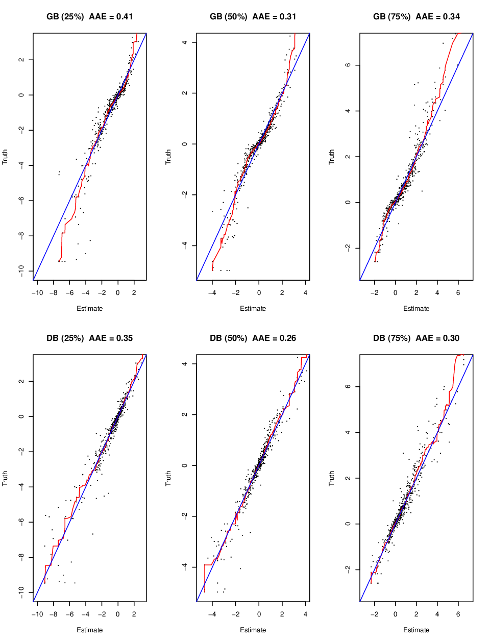
Figure 10 shows true versus predicted values for each of the two methods (rows) on the three quartiles (columns). The red lines represent a running median smooth and the blue lines show equality. The average absolute error associated with each of these plots is
| (22) |
where is the quantity plotted on the horizontal and the vertical axes. The quantile values derived from the estimates of the full distribution (bottom row) are here seen to be somewhat more accurate than those obtained from gradient boosting quantile regression (top row).
With quantile regression each quantile is estimated separately without regard to estimates of other quantiles. Distribution boosting quantile estimates are all derived from a common probability distribution and thus have constraints imposed among them. For example, two quantile estimates have the property for all at any . These constraints can improve accuracy especially when the quantile estimates are being used to compute quantities derived from them.
There is an additional advantage of computing quantities such as means or quantiles from the estimated conditional distributions . As noted in Section 4, distribution contrast trees can be constructed in the presence of arbitrary censoring or truncation. This extends to contrast boosted distribution estimates and any quantities derived from them. This in turn allows application to ordinal regression which can be considered a special case of interval censoring (Friedman 2018).
8 Related work
Regression trees have a long history in Statistics and Machine Learning. Since their first introduction (Morgan and Songquist 1963) many proposed modifications have been introduced to increase accuracy and extend applicability. See Loh (2014) for a nice survey. More recent extensions include Mediboost (Valdes et al 2016) and the Additive Tree (Luna et al 2019). All of these proposals are focused towards estimating the properties of a single outcome variable. There seems to have been little to no work related to applications involving contrasting two variables.
Friedman and Fisher (1999) proposed using tree style recursive partitioning strategies to identify interpretable regions in - space within which the mean of a single outcome was relatively large (“hot spots”). With a similar goal Buja and Lee (2001) proposed using ordinary regression trees with a splitting criterion based on the maximum of the two daughter node means.
Classification tree boosting was proposed by Freund and Schapire (1997). Extension to regression trees was developed by Friedman (2001). Since then there has been considerable research attempting to improve accuracy and extending its scope. See Mayr et al (2014) for a good summary.
Although boosted contrast trees have not been previously proposed they are generally appropriate for the same types of applications as gradient boosted regression trees, such as classification, regression, and quantile regression. They can be beneficial in applications where a contrast tree indicates lack-of-fit of a model produced by some estimation method. In such situations applying contrast boosting to the model predictions often provides improvement in accuracy.
Tree ensembles have also been applied to nonparametric conditional distribution estimation. Meinshausen (2006) used classical random forests to define local neighborhoods in - space. The empirical conditional distribution in each such defined local region around a prediction point is taken as the corresponding conditional distribution estimate at . Athey, Tibshirani and Wagner (2019) noted that since the regression trees used by random forests are designed to detect only mean differences the resulting neighborhoods will fail to adequately capture distributions for which higher moments are not generally functions of the mean. They proposed modified tree building strategies based on gradient boosting ideas to customize random forest tree construction for specific applications including quantile regression.
Boosted regression trees have been used as components in procedures for parametric fitting of conditional distributions and transformations. A parametric form for the conditional distribution or transformation is hypothesized and the parameters as functions of are estimated by regression tree gradient boosting using negative log–likelihood as the prediction risk. See for example Mayr et al (2012), Friedman (2018), Pratola et al (2019), Hothorn (2019) and Mukhopadlhyay & Wang (2019). Some differences between these previous methods and the corresponding approaches proposed here include use of contrast rather than regression trees, and no parametric assumptions.
The principal benefit of the contrast tree based procedures is a lack-of-fit measure. As seen in Table 1 of Section 6.2, and in the Appendix, values of negative log–likelihoods or prediction risk need not reflect actual lack-of-fit to the data. The values of their minima can depend upon other unmeasured quantities. The goal of contrast trees as illustrated in this paper is to provide such a measure. Contrast trees can be applied to assess lack-of-fit of estimates produced by any method, including those mentioned above. If discrepancies are detected, contrast boosting can be employed to remedy them and thereby improve accuracy.
9 Summary
Contrast trees as described in Sections 3 and 4 are designed to provide interpretable goodness-of-fit diagnostics for estimates of the parameters of , or the full distribution. Examples involving classification, probability estimation and conditional distribution estimation were presented in Section 6. A quantile regression example is presented in the Appendix. Two–sample contrast trees for detecting discrepancies between separate data sets are also described in the Appendix.
Boosting of contrast trees is a natural extension. Given an initial estimate from any learning method a contrast tree can assess its goodness or lack-of-fit to the data. If found lacking, the boosting strategy attempts to improve the fit by successively modifying to bring it closer to the data. The Appendix provides an example involving quantile regression where this strategy substantially improved prediction accuracy.
Contrast boosting the full conditional distribution is illustrated on simulated data in Section 7.0.2 and on actual data in the Appendix. Note that the conditional distribution procedure of Section 5.2 can be applied in the presence of arbitrarily censored or truncated data by employing Turnbul’s (1976) algorithm to compute CDFs and corresponding quantiles.
Contrast trees and boosting inherit all of the data analytic advantages of classification and regression trees. These include categorical variables, missing values, invariance to monotone transformations of the predictor variables, resistance to irrelevant predictors, variable importance measures, and few tuning parameters.
Important discussions with Trevor Hastie and Rob Tibshirani on the subject of this work are gratefully acknowledged. An R procedure implementing the methods described herein is available.
References
- [1] Anderson, T. and Darling, D. (1952). Asymptotic theory of certain ”goodness-of-fit” criteria based on stochastic processes. Ann. Stat. 23, 193–212.
- [2] Athey, S., Tibshirani, J., Wagner, S. (2019). Generalized random forests. Ann. Stat. 47(2), 1148-1178.
- [3] Breiman, L., Friedman, J., Olshen, R., and Stone, C. (1984). Classification and Regression Trees. Chapman and Hall.
- [4] Breiman, L. (2001). Random forests. Machine Learning 45, 5-32.
- [5] Buja, A and Lee, Y. (2001). Data mining criteria for tree-based regression and classification. Proceedings of KDD 2001, 27–36.
- [6] Efron, B. (1979). Bootstrap Methods: Another look at the jackknife. Ann. Stat. 7, 1-26.
- [7] Efron, B. and Tibshirani, R. (1994). An Introduction to the Bootstrap. Springer.
- [8] Fernandes, K., Vinagre, P. and Cortez, P. (2015). A proactive intelligent decision support system for predicting the popularity of online news. Proceedings of the 17th EPIA 2015 - Portuguese Conference on Artificial Intelligence. September, Coimbra, Portugal.
- [9] Freund, Y. and Schapire, R. (1997). A decision-theoretic generalization of on-line learning and an application to boosting. J. Computer and System Sciences 55, 119-139.
- [10] Friedman, J. and Fisher, N. (1999) Bump hunting in high-dimensional Data. Statistics and Computing, 9, 123-143.
- [11] Friedman, J. (2001). Greedy function approximation: a gradient boosting machine. Ann. Stat. 29 1189-1232.
- [12] Friedman, J. (2018). Predicting regression probability distributions with imperfect data through optimal transformations. Stanford University Statistics Technical Report.
- [13] Hothorn, T. (2019). Transformation boosting machines. Statistics and Computing. https://doi.org/10.1007/s11222-019-09870-4.
- [14] Kohavi, R. (1996). Scaling up the accuracy of naive-bayes classifiers: a decision-tree hybrid. Proceedings of the Second International Conference on Knowledge Discovery and Data Mining, 1996
- [15] Loh, W. (2014). Fifty years of classification and regression Trees. Inter. Statist. Rev. 82, 3, 329–348.
- [16] Luna, J., Gennatas, E., Eaton, E., Diffenderfer, E., Ungar, L., Jensen, S., Simone, C., Friedman, J., Valdes, G. (2019). The additive tree. Proc. Nat. Acad. Sci.116 (40), 19887-19893.
- [17] Mayr, A., Fenske, N., Hofner, B., Kneib, T., Schmid, M. (2012). GAMLSS for high dimensional data–a flexible approach based on boosting. J. R. Stat. Soc. Ser. C (Appl. Stat) 61(3), 403–427.
- [18] Mayr, A., Binder, H., Gefeller, O., and Schmid, M. (2014). The evolution of boosting algorithms from machine learning to statistical modelling. Methods Inf. Med. 53, 419–427.
- [19] Meinshausen, M. (2006). Quantile random forests. J. Machine Learning Research 7, 983–999.
- [20] Morgan, J. and Sonquist, J. (1963). Problems in the analysis of survey data, and a proposal. J. Amer. Statist. Assoc. 58, 415–434.
- [21] Mukhopadhyay, S. and Wang, K. (2019). On the problem of relevance in statistical inference. J. Amer. Statist. Assoc.(submitted).
- [22] Pratola, M. T., Chipman, H. A, George, E. I., and McCulloch, R. E. (2019). Heteroscedastic BART via multiplicative regression trees, J. of Comput. and Graphical Statist., DOI: 10.1080/10618600.2019.1677243
- [23] Turnbull, B. W. (1976). The empirical distribution function with arbitrarily grouped, censored and truncated data. J. Royal Statist. Soc. B 38, 290-295.
- [24] Valdes, G., Luna, J., Eaton, E., Simone, C , Ungar, L. and Solberg, T. (2016). MediBoost: a patient stratification tool for interpretable decision making in the era of precision medicine. Scientific Reports 6, Article number: 37854.
Appendix
Appendix J Lack-of-fit estimation
Here contrast tree lack-of-fit estimates are compared with known truth on simulated data. There are observations each with predictor variables randomly generated from a standard normal distribution. The outcome is generated from a simple model
with a standard normal random variable. The location and scale functions are given by (17) (18) with different randomly generated parameters. The correlation between the two functions over the data is . The signal/noise is . The goal is to estimate the location function .

Lack-of-fit contrast curves for six methods are shown in Fig. 11. The methods are (top to bottom): black constant fit (global mean), purple single CART tree, blue linear least-squares fit, violet random forest, orange squared-error and red absolute loss gradient boosting. The bottom green curve represents the lack-of-fit contrast curve for the true function on these data. All curves were evaluated on a separate 25000 observation test data set not used to train the respective models.
Table A1
RMS estimation error and contrast tree RMS discrepancy for several methods
Since the data are simulated and truth is here known one can directly compute root-mean-squared estimation error
for each method. This is shown in Table A1 (second column) for each method (first column). The third column shows the root-mean-squared discrepancy over the same test observations calculated from the respective contrast trees for each method. The discrepancy associated with an observation is that of the contrast tree region that contains it.
Contrast tree discrepancy as computed on the data and estimation error based on the (usually unknown) truth are seen here to track each other fairly well. Contrast tree discrepancy is generally smaller that RMS error but relative ratios of the two between the methods are similar.
It is important to note that contrast trees are not perfect. As with any learning method they can sometimes fail to capture sufficiently complex dependencies on the predictor variables . In such situations lack-of-fit may be under estimated. Thus contrast trees can reject fit quality but never absolutely insure it.
Appendix K Quantile regression example
Use of contrast trees in quantile regression is illustrated on the online news popularity data set described in Section 6.3. Here we apply contrast trees to diagnose the accuracy of gradient boosting estimates of the median and th percentile function of .
The usual quantile regression loss used by gradient boosting for estimating the th quantile is given by (21) where here and is the corresponding quantile estimate. With contrast trees we use
| (23) |
as a discrepancy measure. This quantity can be interpreted as prediction error on the probability scale. It is the absolute difference between the target probability and the empirical probability as averaged over the region.
The data were randomly divided into two parts: a learning data set of and and test data set of . A ten region tree to contrast the median of from its gradient boosting predictions was built using (23) on the learning data set and evaluated on the test data set. The results are shown in Fig. 12.

The upper frame shows the empirical (blue) and predicted (red) median in each of the regions in order of absolute discrepancy (23). The lower frame gives the number of counts in each corresponding region. One sees that for 85% of the data (node 20) gradient boosted model predictions of the median appear to be quite close. In other regions of -space there are small to moderate differences.

Figure 13 shows lack-of-fit contrast curves for estimating the median of given by four methods. The green curve represents a constant prediction of the global median at each - value. The red curve is for linear quantile regression. The linear model seems only a little better than the constant one. The black curve represents the gradient boosting predictions based on (21) which are somewhat better. The blue curve is the result of applying contrast boosting (Section 5.1) to the gradient boosting output. Here this strategy appears to substantially improve prediction. For the left most points on each curve the bootstraped errors are respectively , , , and (top to bottom). For the right most points the corresponding errors are , , and . Thus, the larger differences between the curves seen in Fig. 13 are highly significant.

Figure 14 shows lack-of-fit contrast curves for estimating the conditional first quartile () as a function of for the same four methods. Here one sees that the global constant fit appears slightly better that the linear model, while the gradient boosting quantile regression estimate is about twice as accurate. Contrast boosting seems to provide no improvement in this case. Standard errors on the left most points of the respective curves are , , , and (top to bottom). For the right most curves the corresponding errors are , , and .
Table B1
Prediction risk corresponding to the several quantile regression methods for online news data
| Method | Median | 1st Quartile |
| Constant | 2489.5 | 678.3 |
| Linear | 2488.5 | 678.4 |
| Gradient Boosting | 2481.7 | 674.1 |
| Contrast Boosting | 2479.9 | 674.1 |
Table B1 shows quantile regression prediction risk based on loss (21) for median () and first quartile () using the four methods shown in Figs. 13 and 14. Although here prediction risk measures lack-of-accuracy of the methods in the same order as their respective contrast trees, it gives no indication of their actual relative or absolute lack-of-fit to the data as seen from their respective contrast curves in Figs 13 and 14.
Appendix L Distribution boosting example
Distribution boosting is illustrated using the online news popularity data described in Section 6.3. The goal is to estimate the distribution of () popularity of news articles for given sets of predictor variable values . Here we investigate the variation of the final distribution estimate to different initial - distributions . For the same , changing the initial distribution can substantially change the nature of the target transformation functions to be estimated. This can affect ultimate accuracy of the estimates .
Distribution boosting was applied to the observation training data set using three different initial . The first was the same normal distribution at every , where and are the mean and variance of popularity. The second initial distribution, also independent of , is the empirical marginal distribution of as shown in Fig. 15. The third initial - distribution is that of the residual bootstrap at each as described in Section 6.3. This assumes homoscedasticity on the log-scale with varying location.

The upper left frame of Fig. 16 shows the distribution of the average pair-wise difference between the three estimates on each (test set) observation , resulting from the three different beginning - distributions. Difference between two estimates is given by (19) with the evaluation points being a uniform grid between the minimum of quantiles and the maximum of the quantiles of the three distributions.

The 50, 75, and 90 percentiles of the distribution shown in the upper left frame are respectively , , and . As in Fig. 9 the remaining plots in Fig. 16 show the three corresponding s for those observations with pair-wise average difference closest to these respective percentiles. The green curves display the estimate corresponding to the Gaussian starting - distribution, red for the empirical marginal distribution of Fig. 15, and black for the residual bootstrap start. The upper right frame shows that for at least half of the observations the three estimates are fairy similar. The other half exhibit moderate differences. The residual bootstrap estimates tend to be different from the other two, which are usually similar to each other.
Figure 16 shows that different starting - distributions give rise to at least slightly different conditional distribution estimates. In general, different methods produce different answers and one would like to ascertain their respective accuracies. Contrast trees provide a lack-of-fit measure. With conditional distribution estimates one can contrast with on an independent test data set not involved in the estimation as was illustrated in Fig. 5. Here we employ this strategy to evaluate the respective accuracies of the three conditional distribution estimates obtained by the three different starting - distributions.

Figure 17 shows QQ – plots of versus the estimates based on the residual bootstrap starting - distribution. Shown are the nine largest discrepancy regions of a 50 terminal node contrast tree. These nine regions account for 25% of the data. This can be compared to Fig. 5 which shows the corresponding QQ –plots for versus the original residual bootstrap before distribution boosting.

Figure 18 shows the lack-of-fit contrast curves corresponding to the three distribution boosting estimates based on the three different starting - distributions. Each line summarizes a different tree contrasting with one of the corresponding three estimates . The green and red curves in Fig. 18 summarize the results for contrasting with based on the respective Gaussian and empirical marginal distribution (Fig. 15) starting - distributions. Their accuracies are seen to be similar. The black curve summarizes the tree depicted in Fig. 17 contrasting with the estimates based on the residual bootstrap starting - distribution. These estimates appear to be somewhat more accurate. Bootstrap standard errors on the left most points of all three curves are . For the right most points the corresponding errors are , and .
The average discrepancy of the tree contrasting and the residual bootstrap estimated (black) is . The corresponding averages for the respective Gaussian and empirical marginal distribution (Fig. 15) starting - distributions are and respectively. These results can be compared with the discrepancies of their initial untransformed - distributions. Average discrepancy for contrasting with the untransformed residual bootstrap distribution (Fig. 5) is . The corresponding average discrepancies with for the untransformed Gaussian distribution is , and that for the empirical marginal distribution is . Thus the residual bootstrap provided a much closer starting point for estimating ultimately resulting in somewhat more accurate results.
One can obtain a null distribution for average transformed discrepancy by repeatedly applying the contrast boosting procedure with and randomly sampled from the same distribution. In this case and are the same and any differences detected by the distribution boosting procedure, as revealed by a final contrast tree, are caused by the random nature of the data and not actual differences between the respective distributions. Fifty replications of contrasting boosting based on pairs of random samples, each drawn from from the (same) residual bootstrap distribution, produced and average tree discrepancy of with a standard deviation of . Thus there is no evidence here for a systematic difference between the distribution of the original and its estimate based on the residual bootstrap initial - distribution.
Appendix M Two-sample contrast trees
Contrast trees as so far described are applied to a single data set where each observation has two outcomes and , and a single set of predictor variables . A similar methodology can be applied to two–sample problems where there are separate predictor variable measurements for and . Specifically the data consists of two samples and . The predictor values correspond to outcomes , and the values correspond to . The goal to to identify regions in - space where the two conditional distributions and , or selected properties of those distributions, most differ.
Discrepancy measures for each region of - space can be defined in analogy with (1)
| (24) |
Regions and splits are based on the pooled predictor variable sample with . Tree construction strategy is the same as that described in Section 3 using (24).
We illustrate two–sample contrast trees using the census income data set described in Section 6.1. One of the samples is taken to be the data from the 32650 males, and the other sample data from the 16192 females. The goal is to investigate gender differences in probability of high salary (greater than $50K/year, $100K 2020 equivalent) in terms of the other demographic and financial variables as reflected in this data set.
The high salary probability averaged over all males in the data set is whereas that for females is . Thus the relative odds of high salary for men is almost three times that for women over the entire data set. Here we use two–sample contrast trees to investigate whether there are special demographic and financial characteristics for which these relative odds are different. Trees were built on a random half sample of 24421 observations and the corresponding node statistics computed on the other left out half.
We first use two–sample contrast trees to seek regions in predictor variable - space for which male/female relative high salary probability is larger than 3/1. For this we use a ratio discrepancy measure
| (25) |
where represents the males and the females. Here and are indicators of high (male and female) salary and are the corresponding predictor variables.

Figure 19 summarizes results for a ten region contrast tree using (25). In the top frame the height of blue/red bars represent the probability of income greater that $50K for the women/men in the region. In the bottom frame the blue bars represent the fraction of the 16192 women in the region whereas red signifies the corresponding fraction of the 32650 men. The blue/red horizontal lines represent the female/male global average high salary probabilities.
This contrast tree has found several small regions for which the male/female odds ratio (25) is much greater than its global average . For example region 12 containing 551 observations has a 10.3/1 ratio. Region 22 with 501 observations has a 4.6/1 ratio. However, in all of the highest ratio regions the actual male/female probabilities of high salary are well below their respective global averages. In the higher probability regions the ratios roughly correspond to the corresponding global averages.
We next attempt to uncover regions in - space where the female/male high salary odds ratio is much greater than its global average of by using the inverse discrepancy measure

Figure 20 summarizes the regions of the corresponding ten region contrast tree in the same format as Fig. 19. The tree has uncovered three regions in which the high salary probability for women is higher than that for men and much higher than its global average (blue line). In region 12 the female/male high salary odds ratio is 2.6/1. In regions 13 and 11 the probabilities are about equal. In region 11 the overall probability of high salary for both is relatively very high (). This region contains 57% of the males and only 11% of the females in the data set. The rules defining these three regions are
Node 12
age
&
martial status never married
&
hours/week
Node 13
age
&
martial status never married
&
hours/week
Node 11
age
&
martial status never married
&
hours/week
This data set was originally constructed for the purpose of comparing performance of various machine learning algorithms for predicting high salary. There is no information as to its representativeness, even for 1994. The analysis presented here is meant to illustrate the variety of the types of problems to which contrast trees can be applied.
Contrast trees can be used to compare any two samples based on the same measured quantities. In particular, the two samples may be taken from the same system under different conditions or at different times. In these situations contrast trees can detect the presence of any associated “concept drift” between the samples, and if detected explain its nature.