[Uncaptioned image]

Systematically Localizable Operators
for Quantum Simulations of Quantum Field TheoriesPreprint: INT-PUB-19-058

Natalie Klco Email: klcon@uw.edu Affiliation: Institute for Nuclear Theory, University of Washington, Seattle, WA 98195-1550, USA Martin J. Savage Email: mjs5@uw.edu Affiliation: Institute for Nuclear Theory, University of Washington, Seattle, WA 98195-1550, USA

August 11, 2026 - 17:34

Abstract

Correlations and measures of entanglement in ground state wavefunctions of relativistic quantum field theories are spatially localized over length scales set by the mass of the lightest particle. We utilize this localization to design digital quantum circuits for preparing the ground states of lattice scalar quantum field theories. Controlled rotations that are exponentially localized in their position-space extent are found to provide exponentially convergent wavefunction fidelity. These angles scale with the correlation between sites and the classical two-point correlation function, as opposed to the more localized mutual information or the hyper-localized negativity. We anticipate that further investigations will uncover quantum circuit designs with controlled rotations dictated by the measures of entanglement. This work is expected to impact quantum simulations of systems of importance to nuclear physics, high-energy physics, and basic energy sciences research.

I Introduction

Ubiquitous in modern physics, quantum field theories (QFTs) are used to quantitatively describe physical systems from the dynamics of quarks and gluons in the early universe, to the structure of matter in dense astrophysical objects, to the structure and properties of common and exotic materials. The 20th century established the prominence of renormalizable QFTs with local gauge symmetries in describing the strong and electroweak interactions, three of the four fundamental forces in nature. Also at this time effective field theories (EFTs) were established as powerful tools to broadly describe nuclear forces, the properties of hadrons, and lattice regulated field theories over wide kinematic regimes. While significant progress has been made in developing precise analytic frameworks and classical numerical calculations of low-lying observables in non-perturbative systems, other classes of observables—notably real-time dynamics and properties of high density systems—remain to be addressed.

Since the early 1980’s, it has been imagined that the attributes of quantum systems making their at-scale classical computation so onerous will be more naturally represented on quantum computational devices Feynman:1981tf. In quantitative support of this perspective, the complexity class BQP (Bounded Error Quantum Polynomial) has recently been shown to extend beyond the regime of classical polynomial-time calculations Raz:2019:OSB:3313276.3316315. This result indicates that there are problems efficiently accessible to quantum computers but not to classical computers. While the application of quantum computing to scientific applications is only now beginning and it is anticipated that more than a decade of research and development will be required to perform calculations comparable to results of nuclear physics (NP) NPQISrep and high-energy physics (HEP) experiments, there is growing excitement at the prospect of addressing real-time dynamics of highly inelastic processes and the structure of high density systems using quantum computers. Throughout the development toward full-scale quantum simulation, significant physical insight and advances in classical algorithms are expected to emerge that will impact the NP, HEP, and Basic Energy Science (BES) research programs.

Scalar and pseudoscalar fields play key roles in NP, HEP, and BES at both phenomenological and fundamental levels. Perhaps the most famous scalar particle is the $J^{\pi}=0^{+}$ isosinglet $\sigma$ -field (with vacuum quantum numbers), which has been the subject of decades of debate about its nature but is now firmly established Caprini:2005zr. The Higgs boson Higgs:1964pj; Higgs:1964ia has the same quantum numbers as the $\sigma$ , and is the remnant of electroweak symmetry breaking driven by a doublet of complex scalar fields that gives rise to the short-range weak interactions and the long-range electromagnetic interactions Weinberg:1967tq; Glashow:1961tr; Salam:1968rm. Scalar fields also play a central role in phenomenological self-consistent relativistic mean-field theories, providing attractive interactions in the dynamics of large numbers of nucleons (for example, see Ref. Chen:2014sca). Finally, the pion (and kaon) fields are identified as pseudo-Goldstone bosons associated with the spontaneous breaking of the chiral symmetries of quantum chromodynamics (QCD) (for example, see Ref. Weinberg:1978kz). They have been known to be central to NP since the very earliest days and dominate the long-distance behavior of the nucleon-nucleon interaction. In momentum-space, while not required to describe the very low-energy dynamics of nucleon-nucleon (NN) scattering Kaplan:1998we; Kaplan:1998tg; vanKolck:1998bw; Chen:1999tn or low-lying inelastic electroweak processes Chen:1999tn, pions are required to correctly describe processes even at modest energies. Since NN effective field theory (NNEFT) was formulated starting in the early 1990’s Weinberg:1990rz; Ordonez:1992xp; Ordonez:1995rz; vanKolck:1994yi; Kaplan:1998we; Kaplan:1998tg, including both pionless and pionful frameworks, efforts have been ongoing to develop numerical techniques to predict low-energy properties of larger nuclear systems based upon NNEFT systematic power-counting arguments. Explicitly sampling over dynamical pion fields, e.g., with a lattice discretization of spacetime (for example, Refs. Muller:1999cp; Lee:2004si; Abe:2007fe; Lee:2008fa; Lee:2016fhn), constitutes a persisting line of such developments. It is anticipated that quantum simulation of low-energy multi-nuclear systems with dynamical pion fields will provide a quantum advantage in computing real-time dynamics of systems of interest to NP research, e.g., Ref. Holland:2019zju. Therefore, it is timely to develop efficient quantum algorithms and quantum circuits for state preparation and subsequent Hamiltonian time evolution of scalar and (pseudo-)scalar quantum fields on a spatial lattice.

In using quantum computers to predict observables of importance to NP, HEP, and BES research, preparing the initial wave function on the quantum register presents one of the major challenges 2008arXiv0801.0342K; Jordan:2011ne; Jordan:2011ci; Jordan:2014tma; Jordan:2017lea; Preskill2018quantumcomputingin. For example, to determine S-matrix elements of an interacting lattice field theory using the prescription of Jordan, Lee and Preskill (JLP) Jordan:2011ne; Jordan:2011ci; Jordan:2014tma; Jordan:2017lea, localized wave packets of the non-interacting theory are initially prepared. The system is then adiabatically flowed to arrive at localized wave packets in the fully interacting theory, evolved in time through a Trotterized evolution operator, and measured. The final distribution of particles determines the of S-matrix elements of interest. While a perfect initialization would ensure that vacuum fluctuations are accurately captured, an imperfect initialization may allow a background of particles to emerge and evaporate during this process. For example, in calculating the inelastic scattering of two nucleons directly from QCD, a high fidelity preparation of the quantum vacuum is crucial for isolating the process of interest from a complex array of strong interaction backgrounds such as glueballs, pions, and baryon-anti-baryon systems.

Even in the absence of wave packets, preparation of the ground state of the non-interacting lattice field theory remains nontrivial. Focusing on free lattice scalar field theory, the ground state of this coupled system can be defined by $N$ harmonic oscillators, where $N$ is the number of spatial sites of the underlying lattice that discretizes space. Such systems of coupled harmonic oscillators have been considered previously from the view point of quantum information science, including the behavior of mutual information and negativity, e.g. Ref. Anders:2008a. It is most easily represented as the tensor product of the ground state wavefunctions of each of the momentum eigenstates, which can be Fourier transformed into position space. Correspondingly, this wavefunction is the sum over products of oscillator states, one at each spatial site, coupled through the gradient operator in the Hamiltonian. This leads to a high-dimensional Gaussian wave function in the continuum limit, with a non-diagonal covariance matrix in field space. As the classical and quantum correlations—for instance the two-point function, its inverse and measures of entanglement—fall exponentially with spatial separation, the off-diagonal elements in this covariance matrix fall correspondingly. It is this scaling with separation that allows for a quantum computer to be initialized into the ground state of a lattice field theory with the number of operations scaling as a polynomial in the spatial volume.

In this work, we design localizable quantum circuits to prepare the ground states of lattice scalar field theories, both free and interacting, on digital quantum computers. Building upon the foundational papers of JLP Jordan:2011ne; Jordan:2011ci; Jordan:2014tma; Jordan:2017lea, Somma Somma:2016:QSO:3179430.3179434, and more recent works Klco:2018kyo; Klco:2018zqz; PhysRevLett.121.110504; Klco:2019xro; PhysRevA.99.032306, the required controlled operations in these circuits are organized to correspond to spatial separations between field operators—providing a useful relation between the angles of the controlled rotations and the classical and quantum correlations of the QFT. Before presenting numerical results in interacting $\lambda\phi^{4}$ scalar field theory, much of our paper explores free field theory because a number of helpful analytic results are found. Our results are connected to the growing literature exploring the entanglement in fundamental particle interactions and QFTs Calabrese:2004eu; Reznik:2003mnx; Buividovich:2008yv; Donnelly:2011hn; Casini:2013rba; Radicevic:2014kqa; Ghosh2015; Soni:2015yga; Kharzeev:2017qzs; Cervera-Lierta:2017tdt; Witten:2018lha; Beane:2018oxh; Beane:2019loz; Tu:2019ouv as well as the literature on area-law entanglement scalings and tensor network simulatability PhysRevLett.91.147902; Hastings:2007iok; PhysRevB.76.035114; Schuch:2008zza; Brandao:2014ppa. It is also allows for truncations based upon spatial localization to be systematically implemented at the circuit level, and for the subsequent loss of fidelity in the prepared wave function to be systematically quantified.

II Lattice Scalar Field Theory and Its Correlations

The renormalizable Hamiltonian density describing the dynamics of an interacting real scalar field of mass $m$ is,

\displaystyle{\cal H}

\displaystyle=

\displaystyle{1\over 2}\Pi^{2}+{1\over 2}({\bm{\nabla}}\phi)^{2}+{1\over 2}m^{2}\phi^{2}+{\lambda\over 4!}\phi^{4}\ \ \ .

(1)

where the conjugate momentum operator, $\Pi({\bf x})$ has the standard equal-time commutation relation with the field operator, $\left[\ \phi({\bf x}),\Pi({\bf y})\ \right]=i\delta^{3}({\bf x}-{\bf y})$ . For our purposes, we begin by considering the case of the non-interacting field theory with $\lambda=0$ . In order to numerically evaluate observables in this field theory, space is discretized onto a cubic grid with a distance between adjacent lattice sites on the Cartesian axes of $a$ (the lattice spacing) and extent $L$ in each direction. The number of sites in each spatial direction is $N=L/a$ . In terms of dimensionless quantities and replacing the ${\bm{\nabla}}\phi$ operator with a nearest-site finite-difference approximation, the Hamiltonian density for a d-dimensional non-interacting lattice scalar field theory can be written as,

\displaystyle{\cal H}

\displaystyle\rightarrow

\displaystyle{1\over 2}\ \sum_{\bf j}\left[\ \hat{\Pi}^{2}({\bf j})+\hat{m}^{2}\hat{\phi}^{2}({\bf j})+\sum_{\bm{\mu}}\left(\hat{\phi}({\bf j})-\hat{\phi}({\bf j}+\hat{\bm{\mu}})\right)^{2}\ \right]\ \ \ ,

(2)

where $\hat{\bm{\mu}}$ are unit vectors in the d-spatial dimensions, and the sum over ${\bf j}$ corresponds to the sum over all of the lattice sites. We have introduced $\hat{m}=am$ and $\hat{\phi}$ to denote the dimensionless mass and field operator (using powers of the lattice spacing). Throughout the rest of this work, we will use $\phi$ to denote $\hat{\phi}$ for simplicity in notation. Mapping onto a quantum register requires digitizing $\phi$ at each lattice site. Before addressing such a system it is interesting to consider the ground state of this lattice system with continuous $\phi$ ’s. In the case of periodic boundary conditions (PBCs), $\phi(i,j,k,L,l,m,n,...)=\phi(i,j,k,0,l,m,n,...)$ , where the latin arguments represent spatial variables for the scalar field in arbitrary dimensions that become wrapped periodically in each individual dimension. When working in the field basis defined by the eigenstates of the field operator $\phi$ at each spatial site, the conjugate momentum operator can be replaced with the derivative operator in field space, $\hat{\Pi}\psi(\phi)\rightarrow-i{\partial\over\partial\phi}\psi(\phi)$ .

As the continuum limit is approached, $a\rightarrow 0$ , it is helpful to smear operators over physically relevant lengths scales, and not restrict them to be localized around the lattice spacing Davoudi:2012ya. This smearing will make only perturbatively small changes (suppressed by the extent of the smearing) to the value of observables with support in the infrared, but will modify the calculated value of observables at the scale of the smearing or higher. As such, ${\bm{\nabla}}\phi$ could be replaced by an operator smeared over a range of lattice sites, such as

\displaystyle{\bm{\nabla}}\phi

\displaystyle\rightarrow

\displaystyle w_{1}(\phi({\bf j})-\phi({\bf j}+{\bm{\mu}}))\ +\ w_{2}\ {1\over 2}(\phi({\bf j}-{\bm{\mu}})-\phi({\bf j}+{\bm{\mu}}))\ +\ ...\ \ \ ,

(3)

where values of the coefficients $w_{1,2,...}$ can be chosen to optimize aspects of the subsequent computations.

II.1 Continuous Lattice Scalar Field in One Spatial Dimension

The issues we are addressing in this work can be demonstrated clearly in 1-dimension, and straightforwardly extended to higher dimensions. The lattice Hamiltonian for continuous-field wavefunctions can be written as,

\displaystyle{\cal H}

\displaystyle\rightarrow

\displaystyle\sum_{j}^{N}\ -{1\over 2}{\partial^{2}\over\partial\phi(j)^{2}}+{1\over 2}\hat{m}^{2}\phi^{2}(j)+{1\over 2}\left(\phi(j)-\phi(j+1)\right)^{2}\ \ \ ,

(4)

where the nearest-site finite-difference operator is used to represent ${\bm{\nabla}}\phi$ . The analysis of this lattice system, and those defined in higher dimensions, is well known and can be found in standard texts on lattice field theory. Using PBCs, the mass matrix for this system with more than 2 sites has the form of a circulant matrix with first row,

\left(M^{2}\right)_{1}=\begin{pmatrix}\hat{m}^{2}+2&,-1&,0&\cdots&\cdots&\cdots&\cdots&,-1\\ \end{pmatrix}\ \ \ ,

(5)

and the $N$ eigenstates of ${\cal H}$ are spatial plane waves with momentum, $p_{i}=0,\pm{2\pi\over N},\pm{4\pi\over N},...,+\pi$ , with site dependence $v_{p_{i}}(j)={1\over\sqrt{N}}e^{ip_{i}j}$ . The energy-momentum relation resulting from ${\cal H}$ for these momenta is ${\rm E}_{i}^{2}=\hat{m}^{2}+4\sin^{2}\left({p_{i}\over 2}\right)=\hat{m}^{2}+\hat{p}_{i}^{2}$ , defining the hatted momentum variable as that of periodic lattice momentum with ${\rm E}_{i}$ in lattice units. The first and last squared energy eigenvalues (at the edges of the Brillouin zone) are singly degenerate, while the others are doubly degenerate and correspond to states with $+ve$ and $-ve$ momenta. The vector of fields ${\bm{\phi}}=(\phi(0),\phi(1),...,\phi(N-1))^{T}$ , is related to the (momentum) eigenstates of the $M^{2}$ matrix via ${\bm{\chi}}=V{\bm{\phi}}$ , where $V$ is the matrix of the $v_{p_{i}}(j)$ , with $V.M^{2}.V^{\dagger}={\rm diag}({\rm E}_{i}^{2})={\bf E}^{2}$ . The ground state of the coupled system can be written as a tensor product of harmonic oscillators with energy $E_{i}$ , each in their ground state,

\displaystyle|\psi\rangle_{0}

\displaystyle=

\displaystyle|\psi_{\chi_{0}}\rangle_{0}\otimes|\psi_{\chi_{1}}\rangle_{0}\otimes\cdots\otimes|\psi_{\chi_{N-1}}\rangle_{0}\ \ \ ,

(6)

where

\displaystyle\langle\chi_{0},\chi_{1},..\chi_{N-1}|\psi\rangle_{0}

\displaystyle=

\displaystyle{{\rm det}{\bf E}^{1/4}\over\pi^{N/4}}\ e^{-{1\over 2}{\bm{\chi}}^{T}{\rm\bf E}{\bm{\chi}}}\ \ \ .

(7)

In terms of the eigenstates of $\phi(j)$ , this ground state wavefunction of the lattice fields has the form

\displaystyle\langle\phi_{0},\phi_{1},..\phi_{N-1}|\psi\rangle_{0}

\displaystyle=

\displaystyle{{\rm det}{\bf K}^{1/4}\over\pi^{N/4}}\ e^{-{1\over 2}{\bm{\phi}}^{T}{\bf K}{\bm{\phi}}}\ \ \ ,

(8)

where ${\bf K}=V^{\dagger}{\rm\bf E}V$ , which, in general, has non-zero off-diagonal elements.

II.1.1 Two-Point Correlation Functions and Lattice Artifacts

As a reminder of the impact of finite-volume and finite-lattice-spacing artifacts, we provide the example of the two-point function, ${}_{0}\langle\psi|\ \phi_{i}\ \phi_{j}\ |\psi\rangle_{0}$ , in the ground state, i.e. the vacuum expectation value of field correlations between different lattice sites. The expectation value of the product of field operators in the ground state of the scalar field theory can be related to the ${\bf K}$ matrix defined in Eq. (8) via

${}_{0}\langle\psi\|\ \phi_{\ell}\ \phi_{j}\ \|\psi\rangle_{0}$	$\displaystyle=$	$\displaystyle{1\over 2}{\rm\bf K}^{-1}_{\ell j}\ =\ \sum_{\alpha}\ {V_{\ell\alpha}V_{j\alpha}^{*}\over 2E_{\alpha}}\ =\ {1\over N}\ \sum_{p=-(1-{2\over N})\pi}^{+\pi}\ {e^{ip(\ell-j)}\over 2\sqrt{\hat{m}^{2}+\hat{p}^{2}}}$	(9)
	$\displaystyle\rightarrow$	$\displaystyle\int_{-\pi}^{+\pi}{dp\over 2\pi}\ {e^{ip(\ell-j)}\over 2\sqrt{\hat{m}^{2}+\hat{p}^{2}}}\qquad\qquad\qquad(N=\infty\ \ ,\ \ a\neq 0)$
	$\displaystyle\rightarrow$	$\displaystyle\ {1\over 2\pi}K_{0}(\hat{m}\|\ell-j\|)\qquad\qquad\qquad(N=\infty\ \ ,\ \ a=0)$
	$\displaystyle\rightarrow$	$\displaystyle\sqrt{1\over 8\pi}\ {e^{-\hat{m}\|\ell-j\|}\over\sqrt{\hat{m}\|\ell-j\|}}\qquad\qquad\qquad(N=\infty\ \ ,\ \ a=0\ ,\ \|\ell-j\|\rightarrow\infty)\ ,$

where the last two lines are the well-known results in the infinite volume and spatial continuum limits and $K_{0}(x)$ is a modified Bessel function of the second kind. In numerical computations, finite volume artifacts (which can be represented as sums over periodic images) and finite lattice-spacing artifacts (which correspond to modifications to the ultra-violet behavior of the theory encapsulated in the Symanzik action SYMANZIK1983187) will be present. Figure 1 shows this progression of limits for a non-interacting lattice scalar field theory with $\hat{m}=0.3$ calculated on a lattice with $N=30$ spatial sites.

Figure 1: The ground state expectation value

{}_{0}\langle\psi|\ \phi_{n}\ \phi_{0}\ |\psi\rangle_{0}

for a non-interacting lattice scalar field theory with

\hat{m}=0.3

calculated on

N=30

spatial sites (dark blue points). Also shown are the infinite volume limit with non-zero lattice spacing (dark red points), the infinite volume and continuum limit (dark green curve), and its asymptotic dependence for

\hat{m}n\gg 1

(orange curve).

The parameters used in these calculations are chosen so that the scalar particle is contained in the lattice volume, $\hat{m}N=9\gg 1$ , and that it is light compared with the UV cut off of the theory, $\hat{m}\ll\pi$ . The impact of the PBCs on ${}_{0}\langle\psi|\ \phi_{n}\ \phi_{0}\ |\psi\rangle_{0}$ is clear from the symmetry about the midpoint of the lattice. This figure also shows how the finite-volume, finite-lattice-spacing and large-separation expressions converge to the numerical results. The same methods lead to the infinite-volume, continuum limit of ${\bf K}_{ij}$ ,

\displaystyle{\rm\bf K}_{ij}

\displaystyle\rightarrow

\displaystyle-{\hat{m}\over\pi|i-j|}\ K_{1}(\hat{m}|i-j|)\ \ \ ,

(10)

where $K_{1}(x)$ is a modified Bessel function of the second kind. Appendix provides the 4-site lattice scalar field theory in somewhat more detail, and the extension of this methodology to higher dimensions is well known. ¹¹ 1 In d-dimensions, the energy eigenvalues are related to the scalar mass and momentum through $\displaystyle{\rm E}_{i}$ $\displaystyle=$ $\displaystyle\sqrt{\hat{m}^{2}+4\sum_{\bm{\nu}}\ \sin^{2}\left({p_{i,\nu}\over 2}\right)}\ \ \ ,$ (11) where $\nu$ runs over the spatial dimensions. The momentum-space fields are related to the position-space fields via a discrete Fourier transform $\displaystyle\chi_{\bf p}$ $\displaystyle=$ $\displaystyle{1\over\sqrt{N^{d}}}\ \sum_{\bf j}\ e^{i{\bf p}\cdot{\bf j}}\ \phi({\bf j})\ \ \ ,$ (12) where ${\bf p}={2\pi\over N}{\bf n}$ , where ${\bf n}$ is an d-plet of integers, with each element of the vector ranging from $-N/2+1$ to $+N/2$ .

II.1.2 Entanglement Entropy and Mutual Information

The entanglement entropy of a bipartite quantum system quantifies the correlation between two subsystems, $1$ and $2$ , described by a density operator $\hat{\bm{\rho}}_{1,2}$ , and can be written as,

S(\hat{\bm{\rho}}_{1})=\text{Tr}_{1}\left[\ \hat{\bm{\rho}}_{1}\log\hat{\bm{\rho}}_{1}\ \right]\ \ ,\qquad{\rm where}\qquad\hat{\bm{\rho}}_{1}=\text{Tr}_{2}\left[\ \hat{\bm{\rho}}_{1,2}\ \right]\ \ \ ,

(13)

where $\text{Tr}_{j}\left[\ ...\ \right]$ denotes a partial trace over the states in the Hilbert space of system $j$ . When $\hat{\bm{\rho}}_{1,2}$ represents a pure quantum state, the entanglement entropy is a valid measure of entanglement. The mutual information (MI) is useful in quantifying classical and quantum correlations between two subsystems within a larger pure state, $\hat{\bm{\rho}}_{1,2,3,4,....}$ , in which $\hat{\bm{\rho}}_{1,2}$ is not required, nor expected, to be pure

I(1:2)=S(\hat{\bm{\rho}}_{1})+S(\hat{\bm{\rho}}_{2})-S(\hat{\bm{\rho}}_{1,2})\ \ ,\qquad{\rm where}\qquad\hat{\bm{\rho}}_{1,2}=\text{Tr}_{3,4,...}\left[\ \ \hat{\bm{\rho}}_{1,2,3,4,....}\ \right]\ \ \ .

(14)

Following closely the pioneering work of Srednicki Srednicki:1993im, the entanglement entropy and the MI can be calculated in the ground state of a non-interacting lattice scalar field theory. The reduced density operator associated with the field ${\bm{\phi}}$ and ${\bm{\phi}}^{\prime}$ , for a system defined in Eq. (8), is

\hat{\bm{\rho}}({\bm{\phi}},{\bm{\phi}}^{\prime})\propto\int\text{d}\bm{\phi}\text{d}\bm{\phi}^{\prime}\ \int\text{d}\bar{\bm{\phi}}\exp\left[-\frac{1}{2}\begin{pmatrix}\bm{\phi}&\bar{\bm{\phi}}\end{pmatrix}\mathbf{K}\begin{pmatrix}\bm{\phi}\\ \bar{\bm{\phi}}\end{pmatrix}-\frac{1}{2}\begin{pmatrix}\bm{\phi}^{\prime}&\bar{\bm{\phi}}\end{pmatrix}\mathbf{K}\begin{pmatrix}\bm{\phi}^{\prime}\\ \bar{\bm{\phi}}\end{pmatrix}\right]\ |\bm{\phi}\rangle\langle\bm{\phi}^{\prime}|\ \ \ ,

(15)

where $\bm{\phi}$ and $\bm{\phi}^{\prime}$ have dimensionality equal to the number of lattice sites in the subsystem, and $\bar{\bm{\phi}}$ has dimension equal to the number of remaining lattice sites that are removed via partial tracing. The overall normalization of $\hat{\bm{\rho}}({\bm{\phi}},{\bm{\phi}}^{\prime})$ is not shown as it is not required for calculating the entanglement properties of the state (comprised of determinant factors and $\pi$ ’s that set the trace equal to unity). After integrating over the $\bar{\bm{\phi}}$ lattice sites, the reduced density matrix can be written as, see Appendix ,

\hat{\bm{\rho}}({\bm{\phi}},{\bm{\phi}}^{\prime})\propto\exp\left[-\frac{1}{2}\left(\tilde{\bm{\phi}}^{T}\tilde{\bm{\phi}}+\tilde{\bm{\phi}}^{\prime T}\tilde{\bm{\phi}}^{\prime}\right)+\tilde{\bm{\phi}}^{T}\beta^{\prime}\tilde{\bm{\phi}}^{\prime}\right]\ \ \ .

(16)

The eigenvalues of $\hat{\bm{\rho}}({\bm{\phi}},{\bm{\phi}}^{\prime})$ are characterized by $\beta^{\prime}_{i}$ , the eigenvalues of $\beta^{\prime}$ , by identifying $\hat{\bm{\rho}}({\bm{\phi}},{\bm{\phi}}^{\prime})$ as a tensor product of $n$ one-dimensional density matrices $\hat{\bm{\rho}}_{i}(\tilde{\chi}_{i},\tilde{\chi}^{\prime}_{i})$ , where $n$ is the number of sites in the reduced space. The eigenvalues of $\hat{\bm{\rho}}({\bm{\phi}},{\bm{\phi}}^{\prime})$ are multiplicative combinations of the towers of eigenvalues for the individual oscillators Srednicki:1993im,

\xi_{i}=\frac{\beta^{\prime}_{i}}{1+\sqrt{1-\beta_{i}^{{}^{\prime}2}}}\ \ ,\qquad\lambda_{i,n}=(1-\xi_{i})\xi_{i}^{n}\ \ ,\qquad\qquad\lambda_{\hat{\bm{\rho}}_{1}}(\vec{n})=\prod_{i}\lambda_{i,n_{i}}\ \ \ ,

(17)

where $\lambda_{i,n_{i}}$ is the energy eigenvalue of the $n^{\rm th}$ eigenstate of the $i^{\rm th}$ oscillator characterized by $\beta^{\prime}_{i}$ . From these eigenvalues, the entanglement entropy associated with $\hat{\bm{\rho}}({\bm{\phi}},{\bm{\phi}}^{\prime})$ is

\displaystyle S(\hat{\bm{\rho}})

\displaystyle=

\displaystyle-\sum_{\vec{n}}\lambda_{\hat{\bm{\rho}}}(\vec{n})\log\lambda_{\hat{\bm{\rho}}}(\vec{n})\ =\ -\sum_{i}\left[\log(1-\xi_{i})+\frac{\xi_{i}}{1-\xi_{i}}\log\xi_{i}\right]\ \ .

(18)

From general expressions in Eq. (17) and Eq. (18), the MI between two lattice sites may be determined from a combination of calculations with different partitions of the $\mathbf{K}$ matrix. Figure 2 shows the MI of a free lattice scalar field theory with $\hat{m}=0.3$ .

It is found, not surprisingly, that the MI falls exponentially with the separation between the lattice sites Casini:2009sr. To explore this relation, we re-arrange $\hat{\bm{\rho}}({\bm{\phi}},{\bm{\phi}}^{\prime})$ in such a way to make the inter-site-dependence explicit, and examine the behavior of the MI in the limit of large separation. Retaining only two lattice sites, $0$ and $j$ , it is convenient to write $\hat{\bm{\rho}}({\bm{\phi}},{\bm{\phi}}^{\prime})$ in a way that makes clear its tensor product nature in the limit that the two lattice sites become infinitely separated,

	$\displaystyle\hat{\rho}_{0}(\phi,\phi^{\prime})$	$\displaystyle\propto$	$\displaystyle\exp\left[\ -{1\over 2}\left({\bm{\Phi}}_{0}^{T}{\bm{\Sigma}}_{\infty}{\bm{\Phi}}_{0}+{\bm{\Phi}}_{j}^{T}{\bm{\Sigma}}_{\infty}{\bm{\Phi}}_{j}\ +\ 2{\bm{\Phi}}_{0}^{T}{\bm{\Xi}}_{\infty}{\bm{\Phi}}_{j}\right)\ \right]$
	$\displaystyle{\bm{\Phi}}_{i}^{T}$	$\displaystyle=$	$\displaystyle\left(\phi(i),\phi(i)^{\prime}\right)\ \ ,\ \ {\bm{\Sigma}}_{\infty}\ =\ \left(\begin{array}[]{cc}\gamma_{11}&-\beta_{11}\\ -\beta_{11}&\gamma_{11}\end{array}\right)\ \ ,\ \ {\bm{\Xi}}_{\infty}\ =\ \left(\begin{array}[]{cc}\gamma_{12}&-\beta_{12}\\ -\beta_{12}&\gamma_{12}\end{array}\right)\ \ ,$

where $\gamma_{ab}$ and $\beta_{ab}$ are defined in Appendix , and where $\gamma_{12},\beta_{12}\rightarrow e^{-\hat{m}j}/j^{p}$ at large separation. The perturbative analysis given in that Appendix shows that the leading contribution to the MI vanishes as $I(0:j)\rightarrow e^{-2\hat{m}j}/j^{p^{\prime}}$ for large-separations Casini:2009sr. Notably, the MI falls exponentially faster than the two-point correlation function, i.e. with an argument of $-2\hat{m}j$ as opposed to $-\hat{m}j$ .

II.1.3 Negativity

The negativity Vidal:2002zz is a measure of entanglement quantifying purely-quantum correlations. As its name suggests, the negativity is the sum of all negative eigenvalues of the partially transposed density matrix and may be expressed in terms of the matrix square root

\mathcal{N}(\hat{\bm{\rho}})=\frac{||\hat{\bm{\rho}}^{\Gamma}||_{1}-1}{2}=\frac{\text{Tr}\sqrt{\left(\hat{\bm{\rho}}^{\Gamma}\right)^{2}}-1}{2}=\frac{\sum|\lambda_{i}|-1}{2}=-\sum_{\lambda_{i}<0}\lambda_{i}\ \ ,

(24)

where the $\lambda_{i}$ are eigenvalues of (Hermitian) $\hat{\bm{\rho}}^{\Gamma}$ and the unit trace of $\hat{\bm{\rho}}^{\Gamma}$ has been employed.

As a simple example, in the case of a free lattice scalar field theory defined on only two spatial sites as detailed in Appendix , the two-site negativity is

\mathcal{N}(\hat{\bm{\rho}})=\frac{|{\bf K}_{12}|}{{\bf K}_{11}-|{\bf K}_{12}|+\alpha}\ \ ,\qquad\alpha=\sqrt{\det{\bf K}}\ \ \ ,

(25)

which vanishes when the two sites decouple, ${\bf K}_{12}=0$ .

Refer to caption — Figure 2: The mutual information, $I(0;\hat{r})$ , and correlation matrix, ${\rm\bf K}_{1\hskip 0.81949pt\hat{r}+1}$ , in the ground state of a free one-dimensional lattice scalar field theory with $\hat{m}=0.3$ and $N=80$ lattice sites with PBCs (gold and red bars, respectively). To ”guide the eye”, the white lines show fits of the form $e^{-\hat{m}\hat{r}}$ and $e^{-2\hat{m}\hat{r}}$ . The blue bar corresponds to the negativity, ${\cal N}(\hat{\bm{\rho}}._{0\hat{r}})$ , for ${\bm{\nabla}}\phi$ evaluated with a nearest neighbor finite-difference operator, $s_{1}$ . The green-bars denote ${\cal N}(\hat{\bm{\rho}}_{0\hat{r}})$ with ${\bm{\nabla}}\phi$ evaluated a difference operator defined on sites separated by up to distance $\hat{r}=3$ , $s_{3}$ , as defined in Eq. (26). Both ${\rm\bf K}_{1\hskip 2.84544pt\hat{r}+1}$ and $I(0;\hat{r})$ have contributions from terms that decay faster than their asymptotic behavior, leading to relatively slow approaches to asymptopia.

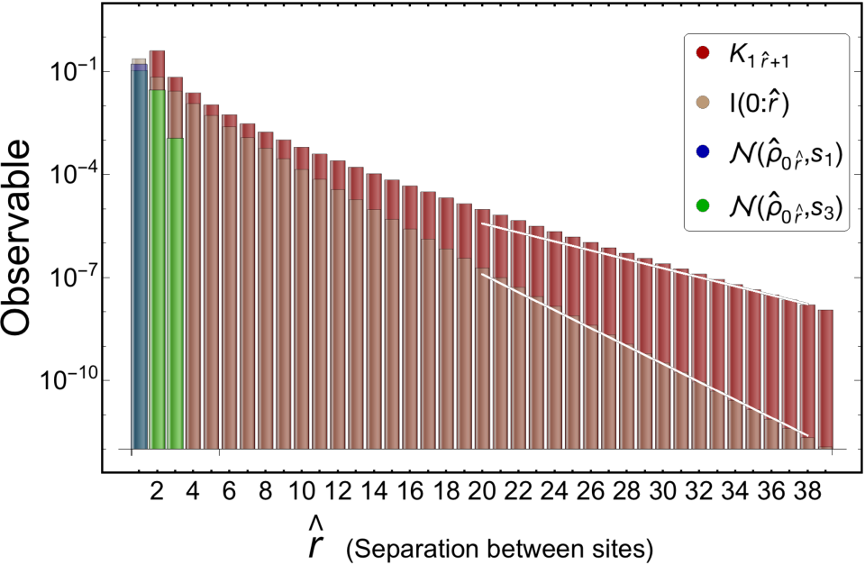
It is interesting to compare $\mathcal{N}(\hat{\bm{\rho}})$ between the fields at two spatial sites with the corresponding MI in a large or infinite lattice scalar field theory. Rather than falling exponentially with spatial separation, $\mathcal{N}(\hat{\bm{\rho}}_{0j})$ is localized to extent of the interaction in the Hamiltonian. In our present calculations, this scale is set by the extent of the finite difference gradient operator used to approximate ${{\bm{\nabla}}\phi}$ in Eq. (1). The forward-difference gradient operator shown in Eq. (4), involving only differences between neighboring sites (denoted by $s_{1}$ ), produces rapidly decaying $\mathcal{N}(\hat{\bm{\rho}})$ , vanishing for all but nearest neighbor negativities. In this light, $\mathcal{N}(\hat{\bm{\rho}})$ is sensitive and characteristic of the ultraviolet properties of the interactions. This behavior has been observed before in systems of coupled harmonic oscillators Anders:2008a. It should be said that for small systems, a small non-zero negativity is found beyond nearest neighbors, but which vanishes rapidly as the extent of the lattices are increased.

To further support these observations, the finite difference operator in Eq. (4) can be modified or smeared to produce different ultraviolet interactions approximating the gradient. For example, the symmetric representation with two-site lattice spacing, ${\bm{\nabla}}\phi\rightarrow\frac{1}{2}\left(\phi({\bf x}+1)-\phi({\bf x}-1)\right)$ , produces non-zero negativities only at two-site spacings. In Fig. 2 we show $\mathcal{N}(\hat{\bm{\rho}}_{0j})$ calculated from a nearest-neighbor-define ${\bm{\nabla}}\phi$ operator, $s_{1}$ , and one defined from sites separated by up to three sites ( $s_{3}$ ),

	$\displaystyle s_{1}:$		$\displaystyle\ ({\bm{\nabla}}\phi(i))^{2}\rightarrow\left(\phi(i+1)-\phi(i)\right)^{2}$
	$\displaystyle s_{3}:$		$\displaystyle\ \left({\bm{\nabla}}\phi(i)\right)^{2}\rightarrow{1\over 3}\left(\phi(i+1)-\phi(i)\right)^{2}\ +\ {1\over 12}\left(\phi(i+2)-\phi(i)\right)^{2}\ +\ {1\over 27}\left(\phi(i+3)-\phi(i)\right)^{2}\ .$		(26)

The negativities associated with $s_{1,3}$ are shown in Fig. 2 as a function of site separation. With such localized quantum correlations manipulatable by varying UV completions, as well as exponentially decaying MI, it is natural to suspect that a logically-designed quantum circuit for initializing the ground state of the scalar field will demonstrate corresponding localization of entangling operators. An explicit digital quantum circuit construction with controlled rotations that are localized on lengths scales set by the classical and quantum correlations that appear in the ${\bf K}$ matrix is the focus of the remainder of this work.

II.2 Digitized Lattice Scalar Field

Determining properties and dynamics of scalar fields on a quantum computer will require digitizing the scalar field at each lattice site Jordan:2011ne; Jordan:2011ci; Jordan:2014tma; Jordan:2017lea. There have been a number of recent studies to quantify such digitization artifacts as understood from the Nyquist-Shannon (NS) Sampling Theorem Somma:2016:QSO:3179430.3179434; Klco:2018kyo; Klco:2018zqz; PhysRevLett.121.110504; Klco:2019xro; PhysRevA.99.032306. It has been shown that, if the field truncation and digitization are informed by NS saturation and correlated in the computational design as qubits are added, the precision of low energy observables can be made to scale double exponentially with the number of qubits used to represent the field at each lattice site. We choose to symmetrically digitize the field at each site, using the basis $\{\ |\phi_{i}\rangle\ \}$ , defined by eigenvectors of the field operator, $\hat{\phi}_{i}$ Klco:2018zqz; Klco:2019xro. For a mapping of each spatial site onto a qubit register of $n_{Q}$ qubits, and hence a Hilbert space of dimensionality $n_{s}=2^{n_{Q}}$ , the Hilbert space of each site in this representation is spanned by $\left\{|-\phi_{\rm max}\rangle\ ,\ |-\phi_{\rm max}+\delta_{\phi}\rangle\ ,\ \cdots,\ |-\frac{\delta_{\phi}}{2}\rangle\ ,\ |\frac{\delta_{\phi}}{2}\rangle\ ,\ \cdots,\ |\phi_{\rm max}-\delta_{\phi}\rangle\ ,\ |\phi_{\rm max}\rangle\right\}$ with field-space lattice spacing $\delta_{\phi}=\frac{2\phi_{\rm max}}{n_{s}-1}$ .

To recover the digitized version of the analytic entangled wave function, it is convenient to start with a wave function with all elements of the lattice-digitized wave functions appearing with equal weight (e.g. a Hadamard operation has been applied to each qubit on each site),

\displaystyle|\psi_{i}\rangle

\displaystyle=

\displaystyle{1\over\sqrt{n_{s}^{N}}}\ \sum_{i_{0},i_{1},\cdots,i_{N-1}=0}^{n_{s}-1}\ |\phi_{0}^{(i_{0})}\rangle\otimes|\phi_{1}^{(i_{1})}\rangle\otimes\cdots\otimes|\phi_{N-1}^{(i_{N-1})}\rangle\ .

(27)

We then define a non-unitary operator from Eq. (8),

\displaystyle\hat{\Gamma}

\displaystyle=

\displaystyle e^{-{1\over 2}\hat{\bm{\phi}}^{T}{\bf K}\hat{\bm{\phi}}}\ \ \ ,

(28)

that reproduces the wave function, once appropriately normalized, in the continuum. The digitized wave function is defined as

\displaystyle|\psi_{d}\rangle

\displaystyle=

\displaystyle A\hat{\Gamma}|\psi_{i}\rangle\ \ \ ,

(29)

where $A$ is the normalization constant, that produces a real wave function across the Hilbert space. The operator is invariant under the symmetry ${\bm{\phi}}\rightarrow-{\bm{\phi}}$ , and hence the $n_{s}^{N}-1$ independent real numbers is reduced to ${1\over 2}n_{s}^{N}-1$ independent real numbers due to the reflection symmetry in field space.

III Quantum Circuits for Ground State Wavefunctions

The following reminds the reader of a generic quantum circuit for preparing wavefunctions with real amplitudes, and introduces a systematic restructuring of the operators to naturally embed localized correlations. The restructuring begins by (at most) doubling the number of quantum operations, in the process making manifest the physically-intuitive removal of long-distance circuit elements. For the lattice scalar field ground state, where two-point correlation functions decay exponentially with separation, this localization allows for truncations of the quantum circuit to approximate the ground state with exponentially improvable fidelity. More generally, this restructuring is expected to be advantageous for position-space qubit representations of field theories exhibiting cluster decomposition or for generic quantum states where classical and/or quantum correlations are suppressed with distance e.g., separation on physical hardware.

III.1 Controlled Rotations: the $\theta$ -Angles

In a previous works 2008arXiv0801.0342K; Quantumc53:online; Klco:2019xro, circuits have been established to prepare an arbitrary real, positive wavefunction with a focus on gaussian-distributed amplitudes. The following circuit is reproduced from Ref. Klco:2019xro,

|\psi\rangle=\quad\begin{gathered}\scalebox{0.9}{ \lx@xy@svg{\hbox{}} \qquad, \qquad\begin{gathered}\end{gathered}\end{gathered}}

Systematically Localizable Operators for Quantum Simulations of Quantum Field TheoriesPreprint: INT-PUB-19-058