跳到论文正文
W Papers独立论文阅读器 arXiv:1912.03550 论文正文 计算阅读时间 · 0%
引用这篇论文根据当前论文元数据生成,正式投稿前建议核对。


License: arXiv.org perpetual non-exclusive license
arXiv:1912.03550v4 [math.OC] 03 Sep 2020

​​​​​​​​​​​​​​​​​​​​​​​​​​​​​​ Minimax Adaptive Control for State Matrix with Unknown SignThe author is a member of the excellence center ELLIIT. Financial support was obtained from the Swedish Research Council and the European Research Council (ERC) Advanced Grant No.834142 (ScalableControl). The work was also partially supported by the Wallenberg AI, Autonomous Systems and Software Program (WASP) funded by the Knut and Alice Wallenberg Foundation.

Anders Rantzer Address: Lund University, Sweden (e-mail: rantzer@control.lth.se).
Abstract

For linear time-invariant systems having a state matrix with uncertain sign, we formulate and solve a minimax adaptive control problem as a zero sum dynamic game. Explicit expressions for the optimal value function and the optimal control law are given in terms of a Riccati equation. The optimal control law is adaptive in the sense that past data is used to estimate the uncertain sign for prediction of future dynamics. Once the sign has been estimated, the controller behaves like standard H∞H_{\infty} optimal state feedback.

keywords
Adaptive control, linear systems, robust control, game theory
 

1 Introduction

The history of adaptive control dates back at least to aircraft autopilot development in the 1950s. Following the landmark paper Åström and Wittenmark 1973, a surge of research activity during the 1970s derived conditions for convergence, stability, robustness and performance under various assumptions. For example, Ljung 1977 analysed adaptive algorithms using averaging, Goodwin et al. 1981 derived an algorithm that gives mean square stability with probability one, while Guo 1995 analyzed the optimal asymptotic rate of convergence. On the other hand, conditions that may cause instability were studied in Egardt 1979, Ioannou and Kokotovic 1984 and Rohrs et al. 1985. Altogether, the subject has a rich history documented in numerous textbooks, such as Åström and Wittenmark 2013, Goodwin and Sin 2014, Sastry and Bodson 2011 and Astolfi et al. 2007. In this paper, the focus is on worst-case models for disturbances and uncertain parameters, as discussed in Cusumano and Poolla 1988; Sun and Ioannou 1987; Megretski and Rantzer 2003. The “minimax adaptive” paradigm was introduced for linear systems in Didinsky and Basar 1994 and nonlinear systems in Pan and Basar 1998.

This is a update to an earlier version published as Rantzer 2020. That version had an error in the main result, which has now been corrected. The outline of the paper is still the same: Sections 2 introduces notation. Section 3 states the problem and reformulates it as a zero sum dynamic game on standard form. The main results are presented in section 4 together with an example. Concluding remarks are given in section 5, while some technical proofs are deferred to an appendix.


2 Notation

The set of n×mn\times m matrices with real coefficients is denoted ℝn×m\mathbb{R}^{n\times m}. The transpose of a matrix AA is denoted A⊤A^{\top}. For a symmetric matrix A∈ℝn×nA\in\mathbb{R}^{n\times n}, we write A≻0A\succ 0 to say that AA is positive definite, while A⪰0A\succeq 0 means positive semi-definite. For A,B∈ℝn×mA,B\in\mathbb{R}^{n\times m}, the expression ⟨A,B⟩\langle A,B\rangle denotes the trace of A⊤​BA^{\top}B. Given x∈ℝnx\in\mathbb{R}^{n} and A∈ℝn×nA\in\mathbb{R}^{n\times n}, the notation |x|A2|x|^{2}_{A} means x⊤​A​xx^{\top}Ax. Similarly, given B∈ℝm×nB\in\mathbb{R}^{m\times n} and A∈ℝn×nA\in\mathbb{R}^{n\times n}, the trace of B⊤​A​BB^{\top}AB is denoted ‖B‖A2\|B\|^{2}_{A}. For y∈ℝy\in\mathbb{R}, define sat⁡(y)\sat(y) to be 11 if y>1y>1 and −1-1 if y<−1y<-1, otherwise equal to yy.

3 Minimax Adaptive Control

This paper is devoted to the following problem:

Let Q∈ℝn×nQ\in\mathbb{R}^{n\times n} and R∈ℝm×mR\in\mathbb{R}^{m\times m} be positive definite matrices and let B∈ℝn×mB\in\mathbb{R}^{n\times m}. Given A∈ℝn×nA\in\mathbb{R}^{n\times n}, and a number γ>0\gamma>0, find, if possible, a control law μ\mu that for every initial state x0x_{0} attains the infimum

infμsupw,i,N∑t=0N(|xt|Q2+|​ut|R2−γ2​|wt|2),\displaystyle\inf_{\mu}\sup_{w,i,N}\sum_{t=0}^{N}\left(|x_{t}|_{Q}^{2}+|u_{t}|_{R}^{2}-\gamma^{2}|w_{t}|^{2}\right), (1)

where i∈{−1,1}i\in\{-1,1\}, wt∈ℝnw_{t}\in\mathbb{R}^{n}, N≥0N\geq 0 and the sequences xx and uu are generated according to

xt+1\displaystyle x_{t+1} =i​A​xt+B​ut+wt\displaystyle=iAx_{t}+Bu_{t}+w_{t} t\displaystyle t ≥0\displaystyle\geq 0 (2)
ut\displaystyle u_{t} =μt​(x0,…,xt,u0,…,ut−1).\displaystyle=\mu_{t}(x_{0},\ldots,x_{t},u_{0},\dots,u_{t-1}). (3)

The problem can be viewed as a dynamic game, where the μ\mu-player tries to minimize the cost, while the (w,i)(w,i)-player tries to maximize it. If it wasn’t for the parameter ii, this would be the standard game formulation of H∞H_{\infty} optimal control Basar and Bernhard 1995. In our formulation, the maximizing player can choose not only ww, but also the parameter ii. This parameter is unknown, but constant, so an optimal feedback law tends to “learn” the value of ii in the beginning, in order to exploit this knowledge later. Such nonlinear adaptive controllers can stabilize and optimize the behavior also when no linear controller can simultaneously stabilize (2) for both i=1i=1 and i=−1i=-1.

To accommodate the uncertainty in ii when deciding utu_{t}, we will see that it is sufficient for the controller to consider historical data collected in the matrix

Zt\displaystyle Z_{t} =∑τ=0t−1[B​uτ−xτ+1xτ]​[B​uτ−xτ+1xτ]⊤.\displaystyle=\sum_{\tau=0}^{t-1}{\begin{bmatrix}Bu_{\tau}-x_{\tau+1}\\ x_{\tau}\end{bmatrix}\begin{bmatrix}Bu_{\tau}-x_{\tau+1}\\ x_{\tau}\end{bmatrix}^{\top}}. (4)

This gives ‖[I​i​A]⊤‖Zt2=∑τ=0t−1|wτ|2\big\|\begin{bmatrix}I\;\;\,iA\end{bmatrix}^{\top}\big\|^{2}_{Z_{t}}=\sum_{\tau=0}^{t-1}|w_{\tau}|^{2} and our problem can be reformulated as follows:

Given Q≻0,R≻0Q\succ 0,R\succ 0, γ>0\gamma>0 and a system

{xt+1=vtZt+1=Zt+[B​ut−vtxt]​[B​ut−vtxt]⊤,Z0=0,\displaystyle\left\{\begin{array}[]{ll}x_{t+1}=v_{t}\\ Z_{t+1}=Z_{t}+{\begin{bmatrix}Bu_{t}-v_{t}\\ x_{t}\end{bmatrix}\begin{bmatrix}Bu_{t}-v_{t}\\ x_{t}\end{bmatrix}^{\top}},&Z_{0}=0,\end{array}\right.

find, if possible, a control law

ut\displaystyle u_{t} =η⁡(xt,Zt)\displaystyle=\eta(x_{t},Z_{t}) (7)

that attains the infimum

infηsupv,N[∑t=0N(|xt|Q2+|​ut|R2)−γ2​mini​‖[I​i​A]⊤‖ZN+12]\displaystyle\!\!\!\!\!\inf_{\eta}\sup_{v,N}\Bigg[\sum_{t=0}^{N}\left(|x_{t}|_{Q}^{2}+|u_{t}|_{R}^{2}\right)-\gamma^{2}\min_{i}\big\|\begin{bmatrix}I\;\;\,iA\end{bmatrix}^{\top}\big\|^{2}_{Z_{N+1}}\Bigg] (8)

when x,u,Zx,u,Z are generated from vv and x0x_{0} using (3)-(7).

In this formulation, the unknown sign ii does not appear in the dynamics, only in the penalty of the final state. As a consequence, no past states are needed in the control law (7), only the state (xt,Zt)(x_{t},Z_{t}). In fact, the problem is a standard zero-sum dynamic game Basar and Olsder 1999, which will next be addressed by dynamic programming.

4 Minimax Dynamic Programming

Define the Bellman operator V↦ℱ​VV\mapsto\mathcal{F}V by

ℱ​V​(x,Z):=\displaystyle\mathcal{F}V(x,Z):=
minu⁡maxv​{|x|Q2+|u|R2+V⁡(v,Z+[B​u−vx]​[B​u−vx]⊤)}\displaystyle\min_{u}\max_{v}\left\{|x|_{Q}^{2}+|u|_{R}^{2}+V\biggl(v,Z+{\begin{bmatrix}Bu-v\\ x\end{bmatrix}\begin{bmatrix}Bu-v\\ x\end{bmatrix}^{\top}}\biggr)\right\}

Then the following results holds:

Theorem 1

Given A,B,Q,RA,B,Q,R, define the operator ℱ\mathcal{F} as above and V0,V1,V2​…V_{0},V_{1},V_{2}\ldots according to the iteration

V0​(x,Z)\displaystyle V_{0}(x,Z) =−γ2​mini=±1​‖[I​i​A]⊤‖Z2\displaystyle=-\gamma^{2}\min_{i=\pm 1}\big\|\begin{bmatrix}I\;\;\,iA\end{bmatrix}^{\top}\big\|^{2}_{Z} (9)
Vk+1​(x,Z)\displaystyle V_{k+1}(x,Z) =ℱ​Vk​(x,Z)\displaystyle={\mathcal{F}}V_{k}(x,Z) (10)

for x∈ℝnx\in\mathbb{R}^{n} and positive semi-definite Z∈ℝn×nZ\in\mathbb{R}^{n\times n}. The expressions (1) and (8) have finite values if and only if the sequence {Vk​(x,0)}k=0∞\{V_{k}(x,0)\}_{k=0}^{\infty} is upper bounded, in which case the limit V∗:=limk→∞VkV_{*}:=\lim_{k\to\infty}V_{k} exists and V∗​(x0,0)V_{*}(x_{0},0) is equal to the values of (1) and (8). Defining η⁡(x,Z)\eta(x,Z) as the minimizing value of uu in the expression for ℱ​V∗​(x,Z)\mathcal{F}V_{*}(x,Z) gives an optimal η\eta for (8), while the control law μ\mu defined by

μt​(x0,…,xt,u0,…,ut−1)\displaystyle\mu_{t}(x_{0},\ldots,x_{t},u_{0},\dots,u_{t-1})
=η⁡(xt,∑τ=0t−1[B​uτ−xτ+1xτ]​[B​uτ−xτ+1xτ]⊤)\displaystyle=\eta\left(x_{t},\sum_{\tau=0}^{t-1}{\begin{bmatrix}Bu_{\tau}-x_{\tau+1}\\ x_{\tau}\end{bmatrix}\begin{bmatrix}Bu_{\tau}-x_{\tau+1}\\ x_{\tau}\end{bmatrix}^{\top}}\right) (11)

is optimal for (1).

Proof. First note that V1≥V0V_{1}\geq V_{0}, so the sequence V0,V1,V2,…V_{0},V_{1},V_{2},\ldots is monotonically non-decreasing.

For any fixed N≥0N\geq 0, the value of (1) is bounded below by the expression

infμsupw,i∑t=0N(|xt|Q2+|​ut|R2−γ2​|wt|2),\displaystyle\inf_{\mu}\sup_{w,i}\sum_{t=0}^{N}\left(|x_{t}|_{Q}^{2}+|u_{t}|_{R}^{2}-\gamma^{2}|w_{t}|^{2}\right), (12)

where i∈{−1,1}i\in\{-1,1\}, wt∈ℝnw_{t}\in\mathbb{R}^{n} and the sequences xx and uu are generated according to (2)-(3). The value of (12) grows monotonically with NN and (1) is obtained in the limit. A change of variables with vt:=xt+1v_{t}:=x_{t+1} and ZtZ_{t} given by (4) shows that (12) is equal to

infμsupv[∑t=0N(|xt|Q2+|​ut|R2)−γ2​mini​‖[I​i​A]⊤‖ZN+12]\displaystyle\inf_{\mu}\sup_{v}\left[\sum_{t=0}^{N}\left(|x_{t}|_{Q}^{2}+|u_{t}|_{R}^{2}\right)-\gamma^{2}\min_{i}\big\|\begin{bmatrix}I\;\;\,iA\end{bmatrix}^{\top}\big\|^{2}_{Z_{N+1}}\right] (13)

where x,Z,ux,Z,u are generated by (3) combined with (3). Standard dynamic programming shows that the value of (13) is VN+1​(x0,0)V_{N+1}(x_{0},0), where VkV_{k} is defined by (9)-(10). This proves that (1) has a finite value if and only if the sequence {Vk​(x,0)}k=0∞\{V_{k}(x,0)\}_{k=0}^{\infty} is upper bounded and the limit V∗​(x0,0)V_{*}(x_{0},0) is equal to the value of (1). It follows from the relationship Vk​(x,Z)≤Vk​(x,0)V_{k}(x,Z)\leq V_{k}(x,0) for Z⪰0Z\succeq 0, that the limit then exists for all Z⪰0Z\succeq 0 and by Lemma 5 in the Appendix the same holds for all symmetric ZZ.

If (8) is finite, then (13) is bounded above by (8), so also V∗:=limk→∞VkV_{*}:=\lim_{k\to\infty}V_{k} is finite. Conversely, if V∗V_{*} is finite, we may define η⁡(x,Z)\eta(x,Z) as a minimizing value of uu in the expression for ℱ​V∗​(x,Z)\mathcal{F}V_{*}(x,Z). Then define the sequence W0,W1,W2,…W_{0},W_{1},W_{2},\ldots recursively by W0:=V0W_{0}:=V_{0} and

Wk+1\displaystyle W_{k+1} (x,Z):=maxv{|x|Q2+|η(x,Z)|R2\displaystyle(x,Z):=\max_{v}\biggl\{|x|^{2}_{Q}+|\eta(x,Z)|^{2}_{R}
+Wk(v,Z+[B​η​(x,Z)−vx][B​η​(x,Z)−vx]⊤)}.\displaystyle+W_{k}\biggl(v,Z+{\begin{bmatrix}B\eta(x,Z)-v\\ x\end{bmatrix}\begin{bmatrix}B\eta(x,Z)-v\\ x\end{bmatrix}^{\top}}\biggr)\biggr\}.

By dynamic programming,

WN​(x,0)\displaystyle W_{N}(x,0)
=supv[−γ2​mini​‖[I​i​A]⊤‖ZN+12+∑t=0N(|xt|Q2+|​ut|R2)],\displaystyle=\sup_{v}\left[-\gamma^{2}\min_{i}\big\|\begin{bmatrix}I\;\;\,iA\end{bmatrix}^{\top}\big\|^{2}_{Z_{N+1}}\!+\!\sum_{t=0}^{N}\left(|x_{t}|_{Q}^{2}+|u_{t}|_{R}^{2}\right)\right],

where x,Z,ux,Z,u are generated by (3) combined with (7). Hence (8) is bounded above by limk→∞Wk​(x0,0)\lim_{k\to\infty}W_{k}(x_{0},0). The definitions of VkV_{k} and WkW_{k} give by induction V∗≥Wk≥VkV_{*}\geq W_{k}\geq V_{k} for all kk, so limk→∞Wk=V∗\lim_{k\to\infty}W_{k}=V_{*}. This proves that the value of (8) equals V∗​(x0,0)V_{*}(x_{0},0) and η\eta is a minimizing argument. □\Box

Corollary 2

With notation as in Theorem 1, suppose that (1) has a finite value and let V∗:=limk→∞VkV_{*}:=\lim_{k\to\infty}V_{k}. Then the Riccati equation

|x|P2\displaystyle|x|^{2}_{P} =minu⁡maxv​{|x|Q2+|​u|R2−γ2​|A​x+B​u−v|2+|v|P2}\displaystyle=\min_{u}\max_{v}\left\{|x|_{Q}^{2}+|u|_{R}^{2}-\gamma^{2}|Ax+Bu-v|^{2}+|v|^{2}_{P}\right\} (14)

has a solution 0≺P≺γ2​I0\prec P\prec\gamma^{2}I and the sequence defined by

V¯0​(x,Z)\displaystyle\bar{V}_{0}(x,Z) =|x|P2−γ2​mini=±1​‖[I​i​A]⊤‖Z2\displaystyle=|x|^{2}_{P}-\gamma^{2}\min_{i=\pm 1}\big\|\begin{bmatrix}I\;\;\,iA\end{bmatrix}^{\top}\big\|^{2}_{Z} (15)
V¯k+1​(x,Z)\displaystyle\bar{V}_{k+1}(x,Z) =ℱ​V¯k​(x,Z).\displaystyle={\mathcal{F}}\bar{V}_{k}(x,Z). (16)

satisfies V¯0≤V¯1≤⋯≤limk→∞V¯k=V∗\bar{V}_{0}\leq\bar{V}_{1}\leq\cdots\leq\lim_{k\to\infty}\bar{V}_{k}=V_{*}.

Proof. Suppose that (1) has a finite value. By Theorem 1, this implies that the sequence {Vk​(x,0)}k=0∞\{V_{k}(x,0)\}_{k=0}^{\infty} defined by (9)-(10) is upper bounded. Define

Vk+​(x,Z)\displaystyle V_{k}^{+}(x,Z) :=|x|Pk2−γ2​‖[I​A]⊤‖Z2\displaystyle:=|x|^{2}_{P_{k}}-\gamma^{2}\big\|\begin{bmatrix}I\;\;\,A\end{bmatrix}^{\top}\big\|^{2}_{Z}
Vk−​(x,Z)\displaystyle V_{k}^{-}(x,Z) :=|x|Pk2−γ2​‖[I−A]⊤‖Z2,\displaystyle:=|x|^{2}_{P_{k}}-\gamma^{2}\big\|\begin{bmatrix}I\;\;\,-A\end{bmatrix}^{\top}\big\|^{2}_{Z},

where P0=0P_{0}=0 and PkP_{k} is given by the Riccati recursion

|x|Pk+12\displaystyle|x|^{2}_{P_{k+1}} =minu⁡maxv​{|x|Q2+|​u|R2−γ2​|A​x+B​u−v|2+|v|Pk2}.\displaystyle=\min_{u}\max_{v}\left\{|x|_{Q}^{2}+|u|_{R}^{2}-\gamma^{2}|Ax+Bu-v|^{2}+|v|^{2}_{P_{k}}\right\}.

Then Vk​(x,Z)≥max⁡{Vk+​(x,Z),Vk−​(x,Z)}V_{k}(x,Z)\geq\max\{V_{k}^{+}(x,Z),V_{k}^{-}(x,Z)\} for all kk. This is trivial for k=0k=0 and follows by induction for k>0k>0, since ℱ​Vk+1+=Vk+\mathcal{F}V^{+}_{k+1}=V^{+}_{k} and ℱ​Vk+1−=Vk−\mathcal{F}V^{-}_{k+1}=V^{-}_{k}. In the limit, it follows that the limit P=limk→∞PkP=\lim_{k\to\infty}P_{k} exists and

V∗​(x,Z)≥V¯0​(x,Z).\displaystyle V_{*}(x,Z)\geq\bar{V}_{0}(x,Z). (17)

Repeated application of ℱ\mathcal{F} gives V∗=limk→∞V¯kV_{*}=\lim_{k\to\infty}\bar{V}_{k}. □\Box

5 An Explicit Optimal Control Law

The following result specifies a minimax optimal adaptive controller on explicit form for a range of γ\gamma-values.

Theorem 3

Given A∈ℝn×nA\in\mathbb{R}^{n\times n}, B∈ℝn×mB\in\mathbb{R}^{n\times m} and some positive definite Q∈ℝn×nQ\in\mathbb{R}^{n\times n}, R∈ℝm×mR\in\mathbb{R}^{m\times m}, assume that (14) has a solution 0≺P≺γ2​I0\prec P\prec\gamma^{2}I, with minimizing argument u=−K​xu=-Kx. Define the sequence {V¯k}k=0∞\{\bar{V}_{k}\}_{k=0}^{\infty} by (15)-(16). Then the following two conditions are equivalent:

  • (ii)

    The value of (1) is finite and V¯k=V¯1\bar{V}_{k}=\bar{V}_{1} for k≥1k\geq 1.

  • (i​iii)

    The matrix T:=Q+A⊤​(P−1−γ2​I)−1​AT:=Q+A^{\top}(P^{-1}-\gamma^{2}I)^{-1}A satisfies

    (γ2​I−P)​(T−P)−1​(γ2​I−P)\displaystyle(\gamma^{2}I-P)(T-P)^{-1}(\gamma^{2}I-P)
    ⪰(I±B​K​A−1)​(γ2​I−P)​(I±B​K​A−1)⊤.\displaystyle\succeq(I\pm BKA^{-1})(\gamma^{2}I-P)(I\pm BKA^{-1})^{\top}.

    for both the “+” and the “-” sign.

Moreover, if (ii) and (i​iii) hold, then (1) has the minimizing control law

ut\displaystyle u_{t} =sat⁡(γ2​∑τ=0t−1(B​uτ−xτ+1)⊤​A​xτ|xt|T−P2)​K​xt\displaystyle=\sat\left(\frac{\gamma^{2}\sum_{\tau=0}^{t-1}(Bu_{\tau}-x_{\tau+1})^{\top}Ax_{\tau}}{|x_{t}|^{2}_{T-P}}\right)Kx_{t} (18)

and, with notation Y:=γ2​[I0]​Z​[0I]⊤Y:=\gamma^{2}\begin{bmatrix}I&0\end{bmatrix}Z\begin{bmatrix}0&I\end{bmatrix}^{\top}, the limit in Theorem 1 can be written as

V∗​(x,Z)\displaystyle V_{*}(x,Z)
={|x|P2−γ2​mini=±1​‖[Ii​A]‖Z2if ​|⟨A,Y⟩|≥|x|T−P2|x|T2−γ2​‖diag⁡{I,A}‖Z2+⟨A,Y⟩2|​x|T−P−2otherwise.\displaystyle=\begin{cases}|x|^{2}_{P}-\gamma^{2}\min_{i=\pm 1}\left\|\begin{bmatrix}I&iA\end{bmatrix}\right\|_{Z}^{2}\qquad\quad\,\,\,\text{if }|\langle A,Y\rangle|\geq|x|^{2}_{T-P}\\ |x|^{2}_{T}-\gamma^{2}\left\|\diag\{I,A\}\right\|_{Z}^{2}+\langle A,Y\rangle^{2}|x|^{-2}_{T-P}\quad\text{otherwise.}\end{cases}

Remark 5.0. The intuition behind the optimal control law in Theorem 3 is simple: The cases ut=K​xtu_{t}=Kx_{t} and ut=−K​xtu_{t}=-Kx_{t} describe the situation when historical data collected in the expression ∑τ=0t−1(B​uτ−xτ+1)⊤​A​xτ\sum_{\tau=0}^{t-1}(Bu_{\tau}-x_{\tau+1})^{\top}Ax_{\tau} is rich enough to make a reliable estimate about the uncertain parameter ii. This estimate is then used as truth and the corresponding H∞H_{\infty} state feedback control law is applied. In the intermediate case, the historical data does not give a conclusive answer, so the controller gain is down-scaled accordingly.

The proof will be based on Lemma 5-8 in the Appendix.

Proof. First assume (i​iii). We will prove the inequality ℱ​V¯1​(x,Z)≤V¯1​(x,Z)\mathcal{F}\bar{V}_{1}(x,Z)\leq\bar{V}_{1}(x,Z) for all x,Zx,Z, (which together with Corollary 2 implies ℱ​V¯k=V¯1\mathcal{F}\bar{V}_{k}=\bar{V}_{1} also for k≥1k\geq 1). By Lemma 5, we may restrict attention to ZZ of the form

Z\displaystyle Z =γ−2​[0YY⊤0].\displaystyle=\gamma^{-2}\begin{bmatrix}0&Y\\ Y^{\top}&0\end{bmatrix}.

Let u^\hat{u} be defined as in Lemma 7. Then the desired inequality is proved by the following sequence of relationships:

ℱ​V¯1​(x,Z)−|x|Q2\displaystyle\mathcal{F}\bar{V}_{1}(x,Z)-|x|_{Q}^{2}
=minu⁡maxv​{|u|R2+V¯1​(v,Z+[B​u−vx]​[B​u−vx]⊤)}\displaystyle=\min_{u}\max_{v}\left\{|u|_{R}^{2}+\bar{V}_{1}\biggl(v,Z+{\begin{bmatrix}Bu-v\\ x\end{bmatrix}\begin{bmatrix}Bu-v\\ x\end{bmatrix}^{\top}}\biggr)\right\}
≤|u^|R2+maxv⁡V¯1​(v,Z+[B​u^−vx]​[B​u^−vx]⊤)\displaystyle\leq|\hat{u}|_{R}^{2}+\max_{v}\bar{V}_{1}\biggl(v,Z+{\begin{bmatrix}B\hat{u}-v\\ x\end{bmatrix}\begin{bmatrix}B\hat{u}-v\\ x\end{bmatrix}^{\top}}\biggr)
=maxvmax|θ|≤1{|v|T2−θ2|v|T−P2−γ2|Bu^−v|2−γ2|Ax|2\displaystyle=\max_{v}\max_{|\theta|\leq 1}\Big\{|v|^{2}_{T}-\theta^{2}|v|^{2}_{T-P}-\gamma^{2}|B\hat{u}-v|^{2}-\gamma^{2}|Ax|^{2}
−2γ2θ(Ax)⊤(Bu^−v)−2θ⟨A,Y⟩}\displaystyle\qquad\qquad\qquad\qquad\quad-2\gamma^{2}\theta(Ax)^{\top}(B\hat{u}-v)-2\theta\langle A,Y\rangle\Big\}
=max|θ|≤1{γ4|θAx+Bu^|(γ2​I−T+θ2​T−θ2​P)−12\displaystyle=\max_{|\theta|\leq 1}\Big\{\gamma^{4}|\theta Ax+B\hat{u}|^{2}_{(\gamma^{2}I-T+\theta^{2}T-\theta^{2}P)^{-1}}
−γ2[|Ax|2+|Bu^|2+2θ(Ax)⊤Bu^]−2θ⟨A,Y⟩}\displaystyle\qquad\qquad-\gamma^{2}\big[|Ax|^{2}+|B\hat{u}|^{2}+2\theta(Ax)^{\top}B\hat{u}\big]-2\theta\langle A,Y\rangle\Big\}
=maxi=±1{γ4|iAx+Bu^|(γ2​I−P)−12\displaystyle=\max_{i=\pm 1}\Big\{\gamma^{4}|iAx+B\hat{u}|^{2}_{(\gamma^{2}I-P)^{-1}}
−γ2[|Ax|2+|Bu^|2+2i(Ax)⊤Bu^]−2i⟨A,Y⟩}\displaystyle\qquad\qquad-\gamma^{2}\big[|Ax|^{2}+|B\hat{u}|^{2}+2i(Ax)^{\top}B\hat{u}\big]-2i\langle A,Y\rangle\Big\}
=maxi=±1⁡{|i​A​x+B​u^|(P−1−γ−2​I)−12−2​i​⟨A,Y⟩}\displaystyle=\max_{i=\pm 1}\Big\{|iAx+B\hat{u}|^{2}_{(P^{-1}-\gamma^{-2}I)^{-1}}-2i\langle A,Y\rangle\Big\}
=|u^|R2+maxv,i⁡{|v|P2+|i​A​x+B​u^−v|2−γ2​‖[I​i​A]⊤‖Z2}\displaystyle=|\hat{u}|_{R}^{2}+\max_{v,i}\Big\{|v|^{2}_{P}+|iAx+B\hat{u}-v|^{2}-\gamma^{2}\big\|\begin{bmatrix}I\;\,iA\end{bmatrix}^{\top}\big\|^{2}_{Z}\Big\}
=|u^|R2+maxv⁡V¯0​(v,Z+[B​u^−vx]​[B​u^−vx]⊤)\displaystyle=|\hat{u}|_{R}^{2}+\max_{v}\bar{V}_{0}\left(v,Z+{\footnotesize\begin{bmatrix}B\hat{u}-v\\ x\end{bmatrix}\begin{bmatrix}B\hat{u}-v\\ x\end{bmatrix}^{\top}}\right)
=V¯1​(x,Z)−|x|Q2.\displaystyle=\bar{V}_{1}(x,Z)-|x|_{Q}^{2}.

The first equality is the definition of ℱ\mathcal{F} and the following inequality is trivial. The second equality is an application of Lemma 7. The third equality follows by analytic elimination of vv (Schur complement). The fourth equality is the main one. It follows from Lemma 8 with

C\displaystyle C :=(γ2I−T)−1/2A\displaystyle:=(\gamma^{2}I-T)^{-1/2}A
D\displaystyle D :=(γ2I−T)−1/2BK\displaystyle:=(\gamma^{2}I-T)^{-1/2}BK
M\displaystyle M :=(γ2I−T)−1/2(T−P)(γ2I−T)−1/2\displaystyle:=(\gamma^{2}I-T)^{-1/2}(T-P)(\gamma^{2}I-T)^{-1/2}
c\displaystyle c :=−2​γ−2​(A​x)⊤​B​u^−2​⟨A,Y⟩.\displaystyle:=-2\gamma^{-2}(Ax)^{\top}B\hat{u}-2\langle A,Y\rangle.

Multiplying the matrices

2​I+M−1+M−(I±D​C−1)​(I+M)​(I±D​C−1)⊤\displaystyle 2I+M^{-1}+M-(I\pm DC^{-1})(I+M)(I\pm DC^{-1})^{\top} (19)

by (γ2​I−T)1/2(\gamma^{2}I-T)^{1/2} from left and right gives, after straightforward manipulations detailed in the Appendix,

(γ2​I−P)​(T−P)−1​(γ2​I−P)\displaystyle(\gamma^{2}I-P)(T-P)^{-1}(\gamma^{2}I-P) (20)
−(I±B​K​A−1)​(γ2​I−P)​(I±B​K​A−1)⊤,\displaystyle-(I\pm BKA^{-1})(\gamma^{2}I-P)(I\pm BKA^{-1})^{\top},

so (i​iii) in Lemma 8 follows from the assumption that (i​iii) holds in Theorem 3. The fifth and sixth equalities are trivial algebraic manipulations, while the seventh is the definition of V¯0\bar{V}_{0}. Finally, the eighth equality is the definition of V¯1\bar{V}_{1}, so the implication from (i​iii) to (ii) in Theorem 3 is proved. The expressions for the optimal control law and the optimal cost are given by Lemma 6.

For the opposite implication, consider the same sequence of expressions as before, but with uˇ\check{u} defined as the minimizing argument in the definition of ℱ​V¯1​(x,Z)\mathcal{F}\bar{V}_{1}(x,Z). This gives

ℱ​V¯1​(x,Z)−|x|Q2\displaystyle\mathcal{F}\bar{V}_{1}(x,Z)-|x|_{Q}^{2}
=max|θ|≤1{γ4|θAx+Buˇ|(γ2​I−T+θ2​T−θ2​P)−12\displaystyle=\max_{|\theta|\leq 1}\Big\{\gamma^{4}|\theta Ax+B\check{u}|^{2}_{(\gamma^{2}I-T+\theta^{2}T-\theta^{2}P)^{-1}}
−γ2[|Ax|2+|Buˇ|2+2θ(Ax)⊤Buˇ]−2θ⟨A,Y⟩}\displaystyle\qquad\qquad-\gamma^{2}\big[|Ax|^{2}+|B\check{u}|^{2}+2\theta(Ax)^{\top}B\check{u}\big]-2\theta\langle A,Y\rangle\Big\}
≥maxi=±1{γ4|iAx+Buˇ|(γ2​I−P)−12\displaystyle\geq\max_{i=\pm 1}\Big\{\gamma^{4}|iAx+B\check{u}|^{2}_{(\gamma^{2}I-P)^{-1}}
−γ2[|Ax|2+|Buˇ|2+2i(Ax)⊤Buˇ]−2i⟨A,Y⟩}\displaystyle\qquad\qquad-\gamma^{2}\big[|Ax|^{2}+|B\check{u}|^{2}+2i(Ax)^{\top}B\check{u}\big]-2i\langle A,Y\rangle\Big\}
=|uˇ|R2+maxv⁡V¯0​(v,Z+[B​uˇ−vx]​[B​uˇ−vx]⊤)\displaystyle=|\check{u}|_{R}^{2}+\max_{v}\bar{V}_{0}\left(v,Z+{\footnotesize\begin{bmatrix}B\check{u}-v\\ x\end{bmatrix}\begin{bmatrix}B\check{u}-v\\ x\end{bmatrix}^{\top}}\right)
≥V¯1​(x,Z)−|x|Q2.\displaystyle\geq\bar{V}_{1}(x,Z)-|x|_{Q}^{2}.

Assume that (i​iii) fails. Then, by Lemma 8, there exist xx and ZZ that make the first inequality strict, so (ii) must fail too and the proof is complete. □\Box

As a complement to the previous result, we also give a lower bound on the values of γ\gamma for which a solution exists:

Theorem 4

With A,B,P,Q,R,TA,B,P,Q,R,T as in Theorem 3, (1) has no finite value unless 0≺P≺γ2​I0\prec P\prec\gamma^{2}I and T⪯γ2​IT\preceq\gamma^{2}I.

Proof. Inserting the bound (17) into the right hand side of the Bellman equation gives

V∗​(x,Z)−|x|Q2\displaystyle V_{*}(x,Z)-|x|_{Q}^{2}
≥ℱ​V¯0​(x,Z)−|x|Q2\displaystyle\!\!\!\geq\mathcal{F}\bar{V}_{0}(x,Z)-|x|_{Q}^{2}
=minu⁡maxv,i​{|u|R2+|v|P2−γ2​|i​A​x+B​u−v|2−γ2​‖[I​i​A]⊤‖Z2}\displaystyle\!\!\!=\min_{u}\max_{v,i}\left\{|u|_{R}^{2}+|v|^{2}_{P}-\gamma^{2}|iAx+Bu-v|^{2}-\gamma^{2}\big\|\begin{bmatrix}I\;\;\,iA\end{bmatrix}^{\top}\big\|^{2}_{Z}\right\}
=minu⁡maxi​{|u|R2+|​i​A​x+B​u|S2−γ2​‖[I​i​A]⊤‖Z2}\displaystyle\!\!\!=\min_{u}\max_{i}\left\{|u|_{R}^{2}+|iAx+Bu|^{2}_{S}-\gamma^{2}\big\|\begin{bmatrix}I\;\;\,iA\end{bmatrix}^{\top}\big\|^{2}_{Z}\right\}
≥|x|T−Q2−γ2​‖diag⁡{I,A}⊤‖Z2\displaystyle\!\!\!\geq|x|^{2}_{T-Q}-\gamma^{2}\big\|\diag\{I,A\}^{\top}\big\|^{2}_{Z}

where the second inequality follows from Lemma 6. Inserting the new bound V∗​(x,Z)≥|x|T2−γ2​‖diag⁡{I,A}⊤‖Z2V_{*}(x,Z)\geq|x|_{T}^{2}-\gamma^{2}\big\|\diag\{I,A\}^{\top}\big\|^{2}_{Z} into the Bellman equation in the same way gives

V∗​(x,0)\displaystyle V_{*}(x,0)
≥minu⁡maxv,i​{|x|Q2+|u|R2+|​v|T2−γ2​|B​u−v|2−γ2​|A​x|2}\displaystyle\geq\min_{u}\max_{v,i}\left\{|x|^{2}_{Q}+|u|_{R}^{2}+|v|^{2}_{T}-\gamma^{2}|Bu-v|^{2}-\gamma^{2}|Ax|^{2}\right\}

The last inequality shows that T⪯γ2​IT\preceq\gamma^{2}I, so the proof is complete. □\Box

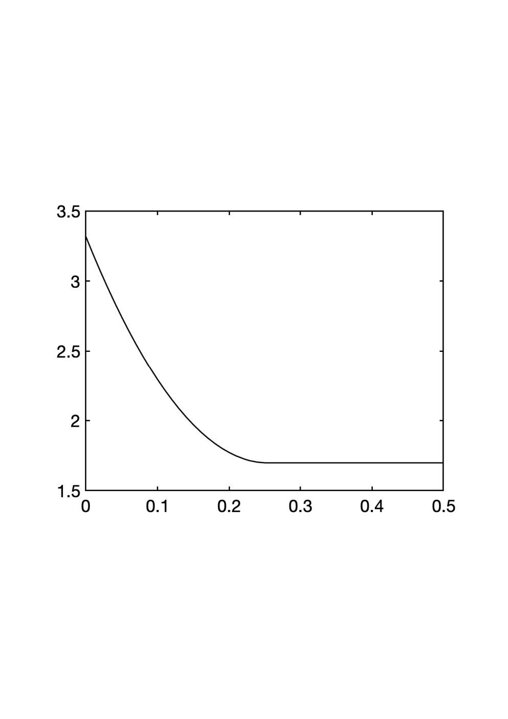
Example 5.0. Consider now the case n=m=Q=R=A=B=1n=m=Q=R=A=B=1. First of all, Theorem 4 shows that the game has no finite value unless γ≥2.01\gamma\geq 2.01. On the other hand, Theorem 3 gives an optimal strategy for the dynamic game (1) whenever γ≥2.5232\gamma\geq 2.5232. Specifically, consider the case γ=2.5232\gamma=2.5232. Solving the Riccati equation gives P=1.6985P=1.6985, which is clearly in the interval [0,γ2][0,\gamma^{2}]. It follows that T=3.3165T=3.3165 and condition (i​iii) of Theorem 3 marginally holds. For larger γ\gamma, the margin would be bigger.

An exact expression for the value function V∗V_{*} is now given by the formula in Theorem 3, which shows that

V∗​(x,[z11z12z12z22])\displaystyle V_{*}\left(x,\begin{bmatrix}z_{11}&z_{12}\\ z_{12}&z_{22}\end{bmatrix}\right)
={1.70​x2−6.37​(z11+z22−2​|z12|)if ​|z12|≥0.25​x23.32​x2−6.37​(z11+z22)+25.05​z122x2otherwise\displaystyle=\begin{cases}1.70x^{2}-6.37(z_{11}+z_{22}-2|z_{12}|)&\text{if }|z_{12}|\geq 0.25x^{2}\\ 3.32x^{2}-6.37(z_{11}+z_{22})+\frac{25.05z_{12}^{2}}{x^{2}}&\text{otherwise}\end{cases}

and the optimal control law is

ut\displaystyle u_{t} =sat⁡(3.93​∑τ=0t−1(uτ−xτ+1)​xτxt2)​0.698​xt.\displaystyle=\sat\left(\frac{3.93\sum_{\tau=0}^{t-1}(u_{\tau}-x_{\tau+1})x_{\tau}}{x_{t}^{2}}\right)0.698x_{t}.

□\Box

Refer to caption

V∗​(1,[zzzz])V_{*}\left(1,\begin{bmatrix}z&z\\ z&z\end{bmatrix}\right)

zz

Figure 1: Optimal value function plot for Example 1. The variable zz represents information about the sign of AA. The cost is maximal for z=0z=0 (no information). For |z|≥0.25|z|\geq 0.25, the cost is the same as if the sign was known.

6 Concluding Remarks

In this paper, we have formulated a control problem for uncertain linear systems as a zero-sum dynamic game. The solution is remarkable for two reasons:

  1. 1.

    The dynamic programming formulation has an explicit solution in terms of a Riccati equation.

  2. 2.

    The resulting optimal controller is adaptive: It reduces the aggressiveness of the controller until until enough data has been collected to get a parameter estimate that can be confidently trusted.

The results are likely to be extendable to many other uncertainty structures. The case of uncertain input matrix BB will be particularly important, since the controller then needs to make active exploration in order to collect enough data for the exploitation phase.

References

  • Astolfi et al. (2007) Alessandro Astolfi, Dimitrios Karagiannis, and Romeo Ortega. Nonlinear and adaptive control with applications. Springer Science & Business Media, 2007.
  • Åström and Wittenmark (1973) Karl Johan Åström and Björn Wittenmark. On self-tuning regulators. Automatica, 9:185–199, January 1973.
  • Åström and Wittenmark (2013) Karl Johan Åström and Björn Wittenmark. Adaptive control. Courier Corporation, 2013.
  • Basar and Bernhard (1995) T. Basar and P. Bernhard. H∞{H}_{\infty}-Optimal Control and Related Minimax Design Problems —A Dynamic Game Approach. Birkhauser, 1995.
  • Basar and Olsder (1999) Tamer Basar and Geert Jan Olsder. Dynamic noncooperative game theory, volume 23. SIAM, 1999.
  • Cusumano and Poolla (1988) Salvatore J Cusumano and Kameshwar Poolla. Nonlinear feedback vs. linear feedback for robust stabilization. In Decision and Control, 1988., Proceedings of the 27th IEEE Conference on, pages 1776–1780. IEEE, 1988.
  • Didinsky and Basar (1994) Garry Didinsky and Tamer Basar. Minimax adaptive control of uncertain plants. In Proceedings of 1994 33rd IEEE Conference on Decision and Control, volume 3, pages 2839–2844. IEEE, 1994.
  • Egardt (1979) Bo Egardt. Stability of Adaptive Controllers. Springer-Verlag, Berlin, FRG, January 1979.
  • Goodwin and Sin (2014) Graham C Goodwin and Kwai Sang Sin. Adaptive filtering prediction and control. Courier Corporation, 2014.
  • Goodwin et al. (1981) Graham C Goodwin, Peter J Ramadge, and Peter E Caines. Discrete time stochastic adaptive control. SIAM Journal on Control and Optim., 19(6):829–853, 1981.
  • Guo (1995) Lei Guo. Convergence and logarithm laws of self-tuning regulators. Automatica, 31(3):435–450, 1995.
  • Ioannou and Kokotovic (1984) Petros A Ioannou and Petar V Kokotovic. Instability analysis and improvement of robustness of adaptive control. Automatica, 20(5):583–594, 1984.
  • Ljung (1977) Lennart Ljung. Analysis of recursive stochastic algorithms. IEEE Transactions on Automatic Control, AC-22:551–575, January 1977.
  • Megretski and Rantzer (2003) A. Megretski and A. Rantzer. Bounds on the optimal ℓ2\ell_{2}-gain in adaptive control of a first order linear system. Technical Report ISRN IML-R–41-02/03–SE+spring, Institut Mittag-Leffler, The Royal Swedish Academy of Sciences, Stockholm, Sweden, January 2003.
  • Pan and Basar (1998) Zigang Pan and Tamer Basar. Adaptive controller design for tracking and disturbance attenuation in parametric strict-feedback nonlinear systems. IEEE Transactions on Automatic Control, 43(8):1066–1083, 1998.
  • Rantzer (2020) Rantzer. Minimax adaptive control for state matrix with unknown sign. In 21th IFAC World Congress, Berlin, Germany, July 2020.
  • Rohrs et al. (1985) C Rohrs, Lena Valavani, Michael Athans, and Gunter Stein. Robustness of continuous-time adaptive control algorithms in the presence of unmodeled dynamics. IEEE Transactions on Automatic Control, 30(9):881–889, 1985.
  • Sastry and Bodson (2011) Shankar Sastry and Marc Bodson. Adaptive control: stability, convergence and robustness. Courier Corporation, 2011.
  • Sun and Ioannou (1987) J Sun and PA Ioannou. The theory and design of robust adaptive controllers. Automatica, pages 19–24, 1987.

Appendix: Supporting Lemmata

The following lemmata are needed for the proof of Theorem 3.

Lemma 5

With the same notation as in Corollary 2, it is true that

V¯k​(x,Z)\displaystyle\bar{V}_{k}(x,Z) =V¯k​(x,Z+diag⁡{Zv​v,Zx​x})\displaystyle=\bar{V}_{k}(x,Z+\diag\{Z_{vv},Z_{xx}\})

for every x∈ℝnx\in\mathbb{R}^{n} and symmetric Z∈ℝ2​n×2​nZ\in\mathbb{R}^{2n\times 2n}, Zv​v∈ℝn×nZ_{vv}\in\mathbb{R}^{n\times n} and Zx​x∈ℝn×nZ_{xx}\in\mathbb{R}^{n\times n}.

Proof. The proof is by induction. The statement is obviously true for k=0k=0. Once it is proved for some value of kk, the formula for ℱ\mathcal{F} gives

V¯k+1​(x,Z+diag⁡{Zv​v,Zx​x}−|x|Q2CLOSE\displaystyle\bar{V}_{k+1}(x,Z+\diag\{Z_{vv},Z_{xx}\}-|x|_{Q}^{2}
=minumaxv{|u|R2+V¯k(v,Z+diag{Zv​v,Zx​x}\displaystyle=\min_{u}\max_{v}\biggl\{|u|_{R}^{2}+\bar{V}_{k}\biggl(v,Z+\diag\{Z_{vv},Z_{xx}\}
+[B​u−vx][B​u−vx]⊤)}\displaystyle\qquad\qquad\qquad\qquad\qquad+{\begin{bmatrix}Bu-v\\ x\end{bmatrix}\begin{bmatrix}Bu-v\\ x\end{bmatrix}^{\top}}\biggr)\biggr\}
=minu⁡maxv​{|u|R2+V¯k​(v,Z+[B​u−vx]​[B​u−vx]⊤)}\displaystyle=\min_{u}\max_{v}\biggl\{|u|_{R}^{2}+\bar{V}_{k}\biggl(v,Z+{\begin{bmatrix}Bu-v\\ x\end{bmatrix}\begin{bmatrix}Bu-v\\ x\end{bmatrix}^{\top}}\biggr)\biggr\}
=V¯k+1​(x,Z)−|x|Q2,\displaystyle=\bar{V}_{k+1}(x,Z)-|x|_{Q}^{2},

so it holds also for k+1k+1. Hence the result follows by induction over kk. □\Box

Lemma 6

Given matrices A,B,YA,B,Y and P,Q,R,S≻0P,Q,R,S\succ 0, suppose that

|x|P2\displaystyle|x|^{2}_{P} =minu⁡{|x|Q2+|​u|R2+|A​x+B​u|S2},\displaystyle=\min_{u}\left\{|x|_{Q}^{2}+|u|_{R}^{2}+|Ax+Bu|^{2}_{S}\right\}, (21)

where the minimizing uu is given by u=−K​xu=-Kx with

K:=(R+B⊤​S​B)−1​B⊤​S​A.\displaystyle K:=(R+B^{\top}SB)^{-1}B^{\top}SA. (22)

Then

minu⁡maxi∈{−1,1}​{|x|Q2+|u|R2+|i​A​x+B​u|S2−2​⟨i​A,Y⟩}\displaystyle\min_{u}\max_{i\in\{-1,1\}}\left\{|x|_{Q}^{2}+|u|_{R}^{2}+|iAx+Bu|^{2}_{S}-2\langle iA,Y\rangle\right\}
={|x|P2+2​|⟨A,Y⟩|if ​|⟨A,Y⟩|≥|x|T−P2|x|T2+⟨A,Y⟩2​|x|T−P−2otherwise\displaystyle=\begin{cases}|x|^{2}_{P}+2|\langle A,Y\rangle|&\text{if }|\langle A,Y\rangle|\geq|x|^{2}_{T-P}\\ |x|^{2}_{T}+\langle A,Y\rangle^{2}|x|^{-2}_{T-P}&\text{otherwise}\end{cases}
=max|θ|≤1⁡{|x|T2−θ2|x|T−P2−2​θ​⟨A,Y⟩},\displaystyle=\max_{|\theta|\leq 1}\left\{|x|^{2}_{T}-\theta^{2}|x|^{2}_{T-P}-2\theta\langle A,Y\rangle\right\},

where T=Q+A⊤​S​AT=Q+A^{\top}SA. The maximizing θ\theta is

θ^\displaystyle\hat{\theta} =−sat⁡(⟨A,Y⟩|x|T−P2)\displaystyle=-\sat\left(\frac{\langle A,Y\rangle}{|x|_{T-P}^{2}}\right)

and the unique minimizing uu is u^=−θ^​K​x\hat{u}=-\hat{\theta}Kx.

Proof. The definition of KK gives

B⊤​S​A\displaystyle B^{\top}SA =(R+B⊤​S​B)​K.\displaystyle=(R+B^{\top}SB)K.

Multiplication by K⊤K^{\top} from the left, and application of the identity

P=Q+K⊤​R​K+(A−B​K)⊤​S​(A−B​K)\displaystyle P=Q+K^{\top}RK+(A-BK)^{\top}S(A-BK)

gives

K⊤​B⊤​S​A=A⊤​S​B​K=K⊤​(R+B⊤​S​B)​K=T−P.\displaystyle K^{\top}B^{\top}SA=A^{\top}SBK=K^{\top}(R+B^{\top}SB)K={T-P}.

The minimax theorem for convex-concave functions gives

minu⁡maxi∈{−1,1}​{|x|Q2+|u|R2+|i​A​x+B​u|S2−2​⟨i​A,Y⟩}\displaystyle\min_{u}\max_{i\in\{-1,1\}}\left\{|x|_{Q}^{2}+|u|_{R}^{2}+|iAx+Bu|^{2}_{S}-2\langle iA,Y\rangle\right\}
=maxθ−1,θ1⁡min⁡∑i∈{−1,1}u⁡θi​{|x|Q2+|u|R2+|i​A​x+B​u|S2−2​⟨i​A,Y⟩}\displaystyle\!\!\!=\max_{\theta_{-1},\theta_{1}}\min_{u}\sum_{i\in\{-1,1\}}\theta_{i}\left\{|x|_{Q}^{2}+|u|_{R}^{2}+|iAx+Bu|^{2}_{S}-2\langle iA,Y\rangle\right\}
=maxθ∈[−1,1]⁡minu​{|x|Q+A⊤​S​A2+|​u|R+B⊤​S​B2+2​θ​(A​x)⊤​S​B​u−2​θ​⟨A,Y⟩}\displaystyle\!\!\!=\max_{\theta\in[-1,1]}\min_{u}\left\{|x|_{Q+A^{\top}SA}^{2}+|u|_{R+B^{\top}SB}^{2}+2\theta(Ax)^{\top}SBu-2\theta\langle A,Y\rangle\right\}
=maxθ∈[−1,1]⁡{|x|T2−θ2|x|T−P2−2​θ​⟨A,Y⟩}\displaystyle\!\!\!=\max_{\theta\in[-1,1]}\left\{|x|^{2}_{T}-\theta^{2}|x|^{2}_{T-P}-2\theta\langle A,Y\rangle\right\}

where θ∈[−1,1]\theta\in[-1,1], θ−1=(1−θ)/2\theta_{-1}=(1-\theta)/2 and θ1=(1+θ)/2\theta_{1}=(1+\theta)/2. If ⟨A,Y⟩≥|x|T−P2\langle A,Y\rangle\geq|x|^{2}_{T-P}, the maximum over θ\theta is attained by θ=−1\theta=-1 and the value is |x|P2+2​⟨A,Y⟩|x|^{2}_{P}+2\langle A,Y\rangle. On the other hand, if ⟨A,Y⟩≤−|x|T−P2\langle A,Y\rangle\leq-|x|^{2}_{T-P}, the maximum is given by θ=1\theta=1 and the value is |x|P2−2​⟨A,Y⟩|x|^{2}_{P}-2\langle A,Y\rangle. Finally, if |⟨A,Y⟩|<|x|T−P2|\langle A,Y\rangle|<|x|^{2}_{T-P}, the optimal value of θ\theta is in the interior of the interval (−1,1)(-1,1) and determined by

|A​x−B​u|S2+2​⟨A,Y⟩\displaystyle|Ax-Bu|^{2}_{S}+2\langle A,Y\rangle =|A​x+B​u|S2−2​⟨A,Y⟩\displaystyle=|Ax+Bu|^{2}_{S}-2\langle A,Y\rangle
⟨A,Y⟩\displaystyle\langle A,Y\rangle =x⊤​A⊤​S​B​u\displaystyle=x^{\top}A^{\top}SBu
=−θ​x⊤​A⊤​S​B​K​x\displaystyle=-\theta x^{\top}A^{\top}SBKx
=−θ​|x|T−P2.\displaystyle=-\theta|x|^{2}_{T-P}.

This gives u=|x|T−P−2​⟨A,Y⟩​K​xu=|x|_{T-P}^{-2}\langle A,Y\rangle Kx and the value

∑iθi​{|x|Q2+|u|R2+|i​A​x+B​u|S2−2​⟨i​A,Y⟩}\displaystyle\sum_{i}\theta_{i}\left\{|x|_{Q}^{2}+|u|_{R}^{2}+|iAx+Bu|^{2}_{S}-2\langle iA,Y\rangle\right\}
=|x|Q2+|u|R2+|​A​x|S2+|​B​u|S2\displaystyle=|x|_{Q}^{2}+|u|_{R}^{2}+|Ax|^{2}_{S}+|Bu|^{2}_{S}
=|x|Q2+|​A​x|S2+|θ​K​x|R+B⊤​S​B2\displaystyle=|x|_{Q}^{2}+|Ax|^{2}_{S}+|\theta Kx|^{2}_{R+B^{\top}SB}
=|x|T2+θ2|​x|T−P2\displaystyle=|x|_{T}^{2}+\theta^{2}|x|^{2}_{T-P}
=|x|T2+⟨A,Y⟩2|​x|T−P−2.\displaystyle=|x|^{2}_{T}+\langle A,Y\rangle^{2}|x|^{-2}_{T-P}.

□\Box

Lemma 7

With the same notation as in Theorem 3 and Y:=γ2​[I0]​Z​[0I]⊤Y:=\gamma^{2}\begin{bmatrix}I&0\end{bmatrix}Z\begin{bmatrix}0&I\end{bmatrix}^{\top}, it is true that

V¯1​(x,Z)\displaystyle\bar{V}_{1}(x,Z)
=maxv⁡{|x|Q2+|u^|R2+V¯0​(v,Z+[B​u^−vx]​[B​u^−vx]⊤)}\displaystyle=\max_{v}\left\{|x|_{Q}^{2}+|\hat{u}|_{R}^{2}+\bar{V}_{0}\biggl(v,Z+{\begin{bmatrix}B\hat{u}-v\\ x\end{bmatrix}\begin{bmatrix}B\hat{u}-v\\ x\end{bmatrix}^{\top}}\biggr)\right\}
=max|θ|≤1⁡{|x|T2−θ2|​x|T−P2−2​θ​⟨A,Y⟩−γ2​‖diag⁡{I,A}⊤‖Z2},\displaystyle=\max_{|\theta|\leq 1}\left\{|x|^{2}_{T}-\theta^{2}|x|^{2}_{T-P}-2\theta\langle A,Y\rangle-\gamma^{2}\big\|\diag\{I,A\}^{\top}\big\|^{2}_{Z}\right\},

where u^=−θ^​K​x\hat{u}=-\hat{\theta}Kx and θ^\hat{\theta} is a maximizing argument of the last expression.

Proof. Define S:=(P−1−γ−2​I)−1S:=(P^{-1}-\gamma^{-2}I)^{-1}. Then

V¯1​(x,Z)−|x|Q2\displaystyle\bar{V}_{1}(x,Z)-|x|_{Q}^{2}
=infusupv{|u|R2+V¯0​(v,Z+[B​u−vx]​[B​u−vx]⊤)}\displaystyle=\inf_{u}\sup_{v}\left\{|u|_{R}^{2}+\bar{V}_{0}\left(v,{Z+\begin{bmatrix}Bu-v\\ x\end{bmatrix}\!\!\begin{bmatrix}Bu-v\\ x\end{bmatrix}^{\top}}\right)\right\}
=minumaxv,i{|u|R2+|v|P2−γ2|iAx+Bu−v|2\displaystyle=\min_{u}\max_{v,i}\Big\{|u|_{R}^{2}+|v|_{P}^{2}-\gamma^{2}|iAx+Bu-v|^{2}
−γ2∥[I​i​A]⊤∥Z2}\displaystyle\qquad\qquad\qquad\qquad\qquad\qquad-\gamma^{2}\big\|\begin{bmatrix}I\;\;iA\end{bmatrix}^{\top}\big\|^{2}_{Z}\Big\}
=minu⁡maxi∈{−1,1}​{|u|R2+|​i​A​x+B​u|S2−γ2​‖[I​i​A]⊤‖Z2}.\displaystyle=\min_{u}\max_{i\in\{-1,1\}}\left\{|u|_{R}^{2}+|iAx+Bu|^{2}_{S}-\gamma^{2}\big\|\begin{bmatrix}I\;\;\,iA\end{bmatrix}^{\top}\big\|^{2}_{Z}\right\}.

so the desired expressions follow from Lemma 6. □\Box

Lemma 8

Given C,D,M∈ℝn×nC,D,M\in\mathbb{R}^{n\times n}, with CC invertible and MM symmetric positive definite, the following statements are equivalent:

  • (ii)

    For every x∈ℝnx\in\mathbb{R}^{n} and c∈ℝc\in\mathbb{R} the maximum

    maxθ∈[−1,1]⁡(|θ​C​x+D​x|(I+θ2​M)−12+θ​c)\displaystyle\max_{\theta\in[-1,1]}\left(|\theta Cx+Dx|^{2}_{(I+\theta^{2}M)^{-1}}+\theta c\right)

    is attained for either θ=−1\theta=-1 or θ=1\theta=1.

  • (i​iii)

    The two matrices

    2​I+M−1+M−(I+D​C−1)​(I+M)​(I+D​C−1)⊤\displaystyle 2I+M^{-1}+M-(I+DC^{-1})(I+M)(I+DC^{-1})^{\top}
    2​I+M−1+M−(I−D​C−1)​(I+M)​(I−D​C−1)⊤\displaystyle 2I+M^{-1}+M-(I-DC^{-1})(I+M)(I-DC^{-1})^{\top}

    are positive semi-definite.

Proof. To prove the lemma, it is convenient to consider two additional statements:

  • (i​i​iiii)

    For all x∈ℝnx\in\mathbb{R}^{n} and θ∈[−1,1]\theta\in[-1,1], it holds that

    |θ​C​x+D​x|(I+θ2​M)−12\displaystyle|\theta Cx+Dx|^{2}_{(I+\theta^{2}M)^{-1}}
    ≤|C​x|(I+M)−12+|​D​x|(I+M)−12+2​θ​x⊤​C⊤​(I+M)−1​D​x.\displaystyle\leq|Cx|^{2}_{(I+M)^{-1}}+|Dx|^{2}_{(I+M)^{-1}}+2\theta x^{\top}C^{\top}(I+M)^{-1}Dx.
  • (i​viv)

    For all x∈ℝnx\in\mathbb{R}^{n} and θ∈[−1,1]\theta\in[-1,1], it holds that

    |θ​C​x+D​x|(I+M−1+θ2​I+θ2​M)−12\displaystyle|\theta Cx+Dx|^{2}_{(I+M^{-1}+\theta^{2}I+\theta^{2}M)^{-1}} ≤|C​x|(I+M)−12.\displaystyle\leq|Cx|^{2}_{(I+M)^{-1}}.

We will first prove that (ii) is equivalent to (i​i​iiii). Define

f⁡(θ)\displaystyle f(\theta) =|θ​C​x+D​x|(I+θ2​M)−12\displaystyle=|\theta Cx+Dx|^{2}_{(I+\theta^{2}M)^{-1}}
g⁡(θ)\displaystyle g(\theta) =|C​x|(I+M)−12+|​D​x|(I+M)−12+2​θ​x⊤​C⊤​(I+M)−1​D​x.\displaystyle=|Cx|^{2}_{(I+M)^{-1}}+|Dx|^{2}_{(I+M)^{-1}}+2\theta x^{\top}C^{\top}(I+M)^{-1}Dx.

Assuming that (i​i​iiii) holds gives

maxθ∈[−1,1]⁡[f⁡(θ)+θ​c]\displaystyle\max_{\theta\in[-1,1]}[f(\theta)+\theta c] ≤maxθ∈[−1,1]⁡[g⁡(θ)+c​θ]\displaystyle\leq\max_{\theta\in[-1,1]}[g(\theta)+c\theta]
=maxθ=±1⁡[g⁡(θ)+c​θ]\displaystyle=\max_{\theta=\pm 1}[g(\theta)+c\theta]
=maxθ=±1⁡[f⁡(θ)+θ​c],\displaystyle=\max_{\theta=\pm 1}[f(\theta)+\theta c],

for all xx, which proves (ii). On the other hand, if (i​i​iiii) fails, there exist a θ^\hat{\theta} and xx such that f⁡(θ^)>g⁡(θ^)f(\hat{\theta})>g(\hat{\theta}). With

c\displaystyle c :=−2​x⊤​C⊤​(I+M)−1​D​x\displaystyle:=-2x^{\top}C^{\top}(I+M)^{-1}Dx

it follows that

f⁡(θ^)+c​θ^\displaystyle f(\hat{\theta})+c\hat{\theta} >g⁡(θ^)+c​θ^\displaystyle>g(\hat{\theta})+c\hat{\theta}
=|C​x|(I+M)−12+|​D​x|(I+M)−12\displaystyle=|Cx|^{2}_{(I+M)^{-1}}+|Dx|^{2}_{(I+M)^{-1}}
=maxθ=±1⁡[g⁡(θ)+c​θ]\displaystyle=\max_{\theta=\pm 1}[g(\theta)+c\theta]
=maxθ=±1⁡[f⁡(θ)+θ​c],\displaystyle=\max_{\theta=\pm 1}[f(\theta)+\theta c],

so also (ii) fails. Hence (ii) is equivalent to (i​i​iiii).

Next, to prove that (i​i​iiii) is equivalent to (i​viv), note that

(I+θ2​M)−1−(I+M)−1\displaystyle(I+\theta^{2}M)^{-1}-(I+M)^{-1}
=(I+θ2​M)−1​[I+M−(I+θ2​M)]​(I+M)−1\displaystyle=(I+\theta^{2}M)^{-1}\left[I+M-(I+\theta^{2}M)\right](I+M)^{-1}
=(1−θ2)​(I+θ2​M)−1​M​(I+M)−1\displaystyle=(1-\theta^{2})(I+\theta^{2}M)^{-1}M(I+M)^{-1}
=(1−θ2)​(I+M−1+θ2​I+θ2​M)−1.\displaystyle=(1-\theta^{2})(I+M^{-1}+\theta^{2}I+\theta^{2}M)^{-1}.

Hence, by subtracting |θ​C​x+D​x|(I+M)−12|\theta Cx+Dx|^{2}_{(I+M)^{-1}} from both sides of the inequality in (i​i​iiii), we get

(1−θ2)​|θ​C​x+D​x|(I+M−1+θ2​I+θ2​M)−12\displaystyle(1-\theta^{2})|\theta Cx+Dx|^{2}_{(I+M^{-1}+\theta^{2}I+\theta^{2}M)^{-1}} ≤(1−θ2)​|C​x|(I+M)−12.\displaystyle\leq(1-\theta^{2})|Cx|^{2}_{(I+M)^{-1}}.

The equivalence between (i​i​iiii) and (i​viv) follows.

It remains to prove that (i​viv) is equivalent to (i​iii). The inequality in (i​viv) holds for all xx if and only if

(θ​C+D)⊤​(I+M−1+θ2​I+θ2​M)−1​(θ​C+D)\displaystyle(\theta C+D)^{\top}(I+M^{-1}+\theta^{2}I+\theta^{2}M)^{-1}(\theta C+D)
⪯C⊤​(I+M)−1​C,\displaystyle\preceq C^{\top}(I+M)^{-1}C,

or equivalently that the matrix

I+M−1+θ2​I+θ2​M−(θ​I+D​C−1)​(I+M)​(θ​I+D​C−1)⊤\displaystyle I+M^{-1}+\theta^{2}I+\theta^{2}M-(\theta I+DC^{-1})(I+M)(\theta I+DC^{-1})^{\top}

is positive semi-definite. The matrix is linear in θ\theta, so the condition holds for all θ∈[−1,1]\theta\in[-1,1] if and only if it holds for θ=±1\theta=\pm 1. Equivalence between (i​viv) and (i​iii) follows. □\Box

Proof of the relationship between (19) and (20).

(γ2​I−T)1/2​(I+M)​(γ2​I−T)1/2\displaystyle(\gamma^{2}I-T)^{1/2}(I+M)(\gamma^{2}I-T)^{1/2}
=γ2​I−T+T−P\displaystyle=\gamma^{2}I-T+T-P
=γ2​I−P\displaystyle=\gamma^{2}I-P
(γ2​I−T)1/2​(I+M−1)​(γ2​I−T)1/2\displaystyle(\gamma^{2}I-T)^{1/2}(I+M^{-1})(\gamma^{2}I-T)^{1/2}
=γ2​I−T+(γ2​I−T)​(T−P)−1​(γ2​I−T)\displaystyle=\gamma^{2}I-T+(\gamma^{2}I-T)(T-P)^{-1}(\gamma^{2}I-T)
=(γ2​I−T)​(T−P)−1​[(T−P)+(γ2​I−T)]\displaystyle=(\gamma^{2}I-T)(T-P)^{-1}\big[(T-P)+(\gamma^{2}I-T)\big]
=(γ2​I−T)​(T−P)−1​(γ2​I−P)\displaystyle=(\gamma^{2}I-T)(T-P)^{-1}(\gamma^{2}I-P)
(γ2​I−T)1/2​(2​I+M+M−1)​(γ2​I−T)1/2\displaystyle(\gamma^{2}I-T)^{1/2}(2I+M+M^{-1})(\gamma^{2}I-T)^{1/2}
=[(T−P)+(γ2​I−T)]​(T−P)−1​(γ2​I−P)\displaystyle=\big[(T-P)+(\gamma^{2}I-T)\big](T-P)^{-1}(\gamma^{2}I-P)
=(γ2​I−P)​(T−P)−1​(γ2​I−P)\displaystyle=(\gamma^{2}I-P)(T-P)^{-1}(\gamma^{2}I-P)
(γ2I−T)1/2(I±DC−1)(γ2I−T)−1/2=I±BKA−1.\displaystyle(\gamma^{2}I-T)^{1/2}(I\pm DC^{-1})(\gamma^{2}I-T)^{-1/2}=I\pm BKA^{-1}.

□\Box