Optimizing Rank-based Metrics with Blackbox Differentiation

Michal Rolínek Thanks: These authors contributed equally. Affiliation: Max-Planck-Institute for Intelligent Systems,Tübingen, Germany Vít Musil Affiliation: Università degli Studi di Firenze,Italy Anselm Paulus Affiliation: Max-Planck-Institute for Intelligent Systems,Tübingen, Germany Marin Vlastelica Affiliation: Max-Planck-Institute for Intelligent Systems,Tübingen, Germany Claudio Michaelis Affiliation: University of Tübingen,Germanymichal.rolinek@tuebingen.mpg.de Georg Martius Affiliation: Max-Planck-Institute for Intelligent Systems,Tübingen, Germany

Abstract

Rank-based metrics are some of the most widely used criteria for performance evaluation of computer vision models. Despite years of effort, direct optimization for these metrics remains a challenge due to their non-differentiable and non-decomposable nature. We present an efficient, theoretically sound, and general method for differentiating rank-based metrics with mini-batch gradient descent. In addition, we address optimization instability and sparsity of the supervision signal that both arise from using rank-based metrics as optimization targets. Resulting losses based on recall and Average Precision are applied to image retrieval and object detection tasks. We obtain performance that is competitive with state-of-the-art on standard image retrieval datasets and consistently improve performance of near state-of-the-art object detectors.

Refer to caption — Figure 1: Differentiation of a piecewise constant rank-based loss. A two-dimensional section of the loss landscape is shown (left) along with two efficiently differentiable interpolations of increasing strengths (middle and right).

1 Introduction

Rank-based metrics are frequently used to evaluate performance on a wide variety of computer vision tasks. For example, in the case of image retrieval, these metrics are required since, at test-time, the models produce a ranking of images based on their relevance to a query. Rank-based metrics are also popular in classification tasks with unbalanced class distributions or multiple classes per image. One prominent example is object detection, where an average over multiple rank-based metrics is used for final evaluation. The most common metrics are recall Ge 2018, Average Precision ( $\ap$ ) Yue et al. 2007, Normalized Discounted Cumulative Gain ( $\ndcg$ ) Chakrabarti et al. 2008, and the Spearman Coefficient Cohendet et al. 2018.

Directly optimizing for the rank-based metrics is inviting but also notoriously difficult due to the non-differentiable (piecewise constant) and non-decomposable nature of such metrics. A trivial solution is to use one of several popular surrogate functions such as 0-1 loss (Lin et al. 2002), the area under the ROC curve (Bartell et al. 1994) or cross entropy. Many studies from the last two decades have addressed direct optimization with approaches ranging from histogram binning approximations Cakir et al. 2019a; Revaud et al. 2019; He et al. 2018a, finite difference estimation Henderson and Ferrari 2016, loss-augmented inference Yue et al. 2007; Mohapatra et al. 2018, gradient approximation Song et al. 2016b all the way to using a large LSTM to fit the ranking operation Engilberge et al. 2019.

Despite the clear progress in direct optimization (Mohapatra et al. 2018; Cakir et al. 2019a; Chen et al. 2019a), these methods are notably omitted in the most publicly used implementation hubs for object detection (Chen et al. 2019b; Wu et al. 2019; Massa and Girshick 2018; Huang et al. 2017), and image retrieval (Roth and Brattoli 2019). The reasons include poor scaling with sequence lengths, lack of publicly available implementations that are efficient on modern hardware, and fragility of the optimization itself.

In a clean formulation, backpropagation through rank-based losses reduces to providing a meaningful gradient of the piecewise constant ranking function. This is an interpolation problem, rather than a gradient estimation problem (the true gradient is simply zero almost everywhere). Accordingly, the properties of the resulting interpolation (whose gradients are returned) should be of central focus, rather than the gradient itself.

In this work, we interpolate the ranking function via blackbox backpropagation Vlastelica et al. 2020, a framework recently proposed in the context of combinatorial solvers. This framework is the first one to give mathematical guarantees on an interpolation scheme. It applies to piecewise constant functions that originate from minimizing a discrete objective function. To use this framework, we reduce the ranking function to a combinatorial optimization problem. In effect, we inherit two important features of Vlastelica et al. 2020: mathematical guarantees and the ability to compute the gradient only with the use of a non-differentiable blackbox implementation of the ranking function. This allows using implementations of ranking functions that are already present in popular machine learning frameworks which results in straightforward implementation and significant practical speed-up. Finally, differentiating directly the ranking function gives additional flexibility for designing loss functions.

Having a conceptually pure solution for the differentiation, we can then focus on another key aspect: sound loss design. To avoid ad-hoc modifications, we take a deeper look at the caveats of direct optimization for rank-based metrics. We offer multiple approaches for addressing these caveats, most notably we introduce margin-based versions of rank-based losses and mathematically derive a recall-based loss function that provides dense supervision.

Experimental evaluation is carried out on image retrieval tasks where we optimize the recall-based loss and on object detection where we directly optimize mean Average Precision. On the retrieval experiments, we achieve performance that is on-par with state-of-the-art while using a simpler setup. On the detection tasks, we show consistent improvement over highly-optimized implementations that use the cross-entropy loss, while our loss is used in an out-of-the-box fashion. We release the code used for our experiments¹¹ 1 https://github.com/martius-lab/blackbox-backprop..

2 Related work

Optimizing for rank-based metrics

As rank-based evaluation metrics are now central to multiple research areas, their direct optimization has become of great interest to the community. Traditional approaches typically rely on different flavors of loss-augmented inference Mohapatra et al. 2018; Yue et al. 2007; Mohapatra et al. 2014; McFee and Lanckriet 2010, or gradient approximation Song et al. 2016b; Henderson and Ferrari 2016. These approaches often require solving a combinatorial problem as a subroutine where the nature of the problem is dependent on the particular rank-based metric. Consequently, efficient algorithms for these subproblems were proposed Mohapatra et al. 2018; Song et al. 2016b; Yue et al. 2007.

More recently, differentiable histogram-binning approximations Cakir et al. 2019a; He et al. 2018a; He et al. 2018b; Revaud et al. 2019 have gained popularity as they offer a more flexible framework. Completely different techniques including learning a distribution over rankings Taylor et al. 2008, using a policy-gradient update rule Rao et al. 2018, learning the sorting operation entirely with a deep LSTM Engilberge et al. 2019 or perceptron-like error-driven updates have also been applied Chen et al. 2019a.

Metric learning

There is a great body of work on metric learning for retrieval tasks, where defining a suitable loss function plays an essential role. Bellet et al. 2013 and Kulis et al. 2013 provide a broader survey of metric learning techniques and applications. Approaches with local losses range from employing pair losses Bromley et al. 1994; Koch et al. 2015, triplet losses Schroff et al. 2015; Hoffer and Ailon 2015; Song et al. 2016b to quadruplet losses Law et al. 2013. While the majority of these works focus on local, decomposable losses as above, multiple lines of work exist for directly optimizing global rank-based losses Engilberge et al. 2019; Taylor et al. 2008; Revaud et al. 2019. The importance of good batch sampling strategies is also well-known, and is the subject of multiple studies Oh Song et al. 2016; Schroff et al. 2015; Ge 2018; Wu et al. 2017, while others focus on generating novel training examples Zhao et al. 2018; Song et al. 2016b; Movshovitz-Attias et al. 2017.

Object detection

Modern object detectors use a combination of different losses during training Girshick et al. 2014; Ren et al. 2015; Liu et al. 2016a; Redmon et al. 2016; He et al. 2017a; Lin et al. 2018. While the biggest performance gains have originated from improved architectures Ren et al. 2015; He et al. 2017a; Redmon and Farhadi 2018; Ghiasi et al. 2019 and feature extractors He et al. 2016; Zoph et al. 2018, some works focused on formulating better loss functions Lin et al. 2018; Rezatofighi et al. 2019; Goldman et al. 2019. Since its introduction in the Pascal VOC object detection challenge Everingham et al. 2010 mean Average Precision ( $\map$ ) has become the main evaluation metric for detection benchmarks. Using the metric as a replacement for other less suitable objective functions has thus been studied in several works Song et al. 2016b; Henderson and Ferrari 2016; Rao et al. 2018; Chen et al. 2019a.

3 Background

3.1 Rank-based metrics

For a positive integer $n$ , we denote by $\Pi_{n}$ the set of all permutations of $\{1,\ldots,n\}$ . The rank of vector $\mathbf{y}=[y_{1},\dots,y_{n}]\in\mathbb{R}^{n}$ , denoted by $\rank(\mathbf{y})$ , is a permutation $\pi\in\Pi_{n}$ satisfying

y_{\pi^{-1}(1)}\geq y_{\pi^{-1}(2)}\geq\cdots\geq y_{\pi^{-1}(n)},

(1)

i.e. sorting $\mathbf{y}$ . Note, that rank is not defined uniquely for those vectors for which any two components coincide. In the formal presentation, we reduce our attention to proper rankings in which ties do not occur.

The rank $\rank$ of the $i$ -th element is one plus the number of members in the sequence exceeding its value, i.e.

\rank(\mathbf{y})_{i}=1+|\{j:y_{j}>y_{i}\}|.

(2)

3.1.1 Average Precision

For a fixed query, let $\mathbf{y}\in\mathbb{R}^{n}$ be a vector of relevance scores of $n$ examples. We denote by $\mathbf{y}^{*}\in\{0,1\}^{n}$ the vector of their ground truth labels (relevant/irrelevant) and by

\rel(\mathbf{y}^{*})=\{i:y^{*}_{i}=1\}

(3)

the set of indices of the relevant examples. Then Average Precision is given by

\ap(\mathbf{y},\mathbf{y}^{*})=\frac{1}{|\rel(\mathbf{y}^{*})|}\sum_{i\in\rel(\mathbf{y}^{*})}\precision(i),

(4)

where precision at $i$ is defined as

\precision(i)=\frac{|\{j\in\rel(\mathbf{y}^{*}):y_{j}\geq y_{i}\}|}{\rank(\mathbf{y})_{i}}

(5)

and describes the ratio of relevant examples among the $i$ highest-scoring examples.

In classification tasks, the dataset typically consists of annotated images. This we formalize as pairs $(x_{i},\mathbf{y}^{*}_{i})$ where $x_{i}$ is an input image and $\mathbf{y}^{*}_{i}$ is a binary class vector, where, for every $i$ , each $(\mathbf{y}^{*}_{i})_{c}\in\{0,1\}$ denotes whether an image $x_{i}$ belongs to the class $c\in\mathcal{C}$ . Then, for each example $x_{i}$ the model provides a vector of suggested class-relevance scores $\mathbf{y}_{i}=\phi(x_{i},\theta)$ , where $\theta$ are the parameters of the model.

To evaluate mean Average Precision ( $\map$ ), we consider for each class $c\in\mathcal{C}$ the vector of scores $\mathbf{y}(c)=[(\mathbf{y}_{i})_{c}]_{i}$ and labels $\mathbf{y}^{*}(c)=[(\mathbf{y}^{*}_{i})_{c}]_{i}$ . We then take the mean of Average Precisions over all the classes

\map=\frac{1}{|\mathcal{C}|}\sum_{c\in\mathcal{C}}\ap\bigl(\mathbf{y}(c),\mathbf{y}^{*}(c)\bigr).

(6)

Note that $\map\in[0,1]$ and that the highest score 1 corresponds to perfect score prediction in which all relevant examples precede all irrelevant examples.

3.1.2 Recall

Recall is a metric that is often used for information retrieval. Let again $\mathbf{y}\in\mathbb{R}^{n}$ and $\mathbf{y}^{*}\in\{0,1\}^{n}$ be the scores and the ground-truth labels for a given query over a dataset. For a positive integer $K$ , we set

\rak(\mathbf{y},\mathbf{y}^{*})=\begin{cases}1&\text{if $\exists i\in\rel(\mathbf{y}^{*})$ with $\rank(\mathbf{y})_{i}\leq K$}\\ 0&\text{otherwise,}\end{cases}

(7)

where $\rel(\mathbf{y}^{*})$ is given in Eq. 3.

In a setup where each element $x_{i}$ of the dataset $\mathcal{D}$ is a possible query, we define the ground truth matrix as follows. We set $\mathbf{y}^{*}_{i}(j)=1$ if $x_{j}$ belongs to the same class as the query $x_{i}$ , and zero otherwise. The scores suggested by the model are again denoted by $\mathbf{y}_{i}=[\phi(x_{i},x_{j},\theta)\colon j\in\mathcal{D}]$ .

In order to evaluate the model over the whole dataset $\mathcal{D}$ , we average $\rak$ over all the queries $x_{i}$ , namely

\Rak=\frac{1}{|\mathcal{D}|}\sum_{i\in\mathcal{D}}\rak\bigl(\mathbf{y}_{i},\mathbf{y}^{*}_{i}\bigr).

(8)

Again, $\Rak\in[0,1]$ for every $K$ . The highest score 1 means that a relevant example is always found among the top $K$ predictions.

3.2 Blackbox differentiation of combinatorial solvers

In order to differentiate the ranking function, we employ a method for efficient backpropagation through combinatorial solvers – recently proposed in (Vlastelica et al. 2020). It turns algorithms or solvers for problems like shortest-path, traveling-salesman-problem, and various graph cuts into differentiable building blocks of neural network architectures.

With minor simplifications, such solvers (e.g. for the Multicut problem) can be formalized as maps that take continuous input $\mathbf{y}\in\mathbb{R}^{n}$ (e.g. edge weights of a fixed graph) and return discrete output $\mathbf{s}\in{S}\subset\mathbb{R}^{n}$ (e.g. indicator vector of a subset of edges forming a cut) such that it minimizes a combinatorial objective expressed as an inner product $\mathbf{y}\cdot\mathbf{s}$ (e.g. the cost of the cut). Note that the notation differs from (Vlastelica et al. 2020) ( $\mathbf{y}$ was $w$ and $\mathbf{s}$ was $y$ ). In short, a blackbox solver is

\mathbf{y}\mapsto\mathbf{s}(\mathbf{y})\quad\text{such that}\quad\mathbf{s}(\mathbf{y})=\argmin_{\mathbf{s}\in{S}}\mathbf{y}\cdot\mathbf{s},

(9)

where ${S}$ is the discrete set of admissible assignments (e.g. subsets of edges forming cuts).

The key technical challenge when computing the backward pass is meaningful differentiation of the piecewise constant function $\mathbf{y}\to L(\mathbf{s}(\mathbf{y}))$ where $L$ is the final loss of the network. To that end, (Vlastelica et al. 2020) constructs a family of continuous and (almost everywhere) differentiable functions parametrized by a single hyperparameter $\lambda>0$ that controls the trade-off between “faithfulness to original function” and “informativeness of the gradient”, see Fig. 1. For a fixed $\lambda$ the gradient of such an interpolation at point $\mathbf{s}$ is computed and passed further down the network (instead of the true zero gradient) as

\displaystyle\frac{\partial L(\mathbf{s}(\mathbf{y}))}{\partial\mathbf{y}}:=-\frac{1}{\lambda}(\mathbf{s}-\mathbf{s}_{\lambda})

(10)

where $\mathbf{s}_{\lambda}$ is the output of the solver for a certain precisely constructed modification of the input. The modification is where the incoming gradient information $\partial L(\mathbf{s}(\mathbf{y}))/{\partial\mathbf{s}(\mathbf{y})}$ is used. For full details including the mathematical guarantees on the tightness of the interpolation, see (Vlastelica et al. 2020).

The main advantage of this method is that only a blackbox implementation of the solver (i.e. of the forward pass) is required to compute the backward pass. This implies that powerful optimized solvers can be used instead of relying on suboptimal differentiable relaxations.

4 Method

4.1 Blackbox differentiation for ranking

In order to apply blackbox differentiation method for ranking, we need to find a suitable combinatorial objective. Let $\mathbf{y}\in\mathbb{R}^{n}$ be a vector of $n$ real numbers (the scores) and let $\rank\in\Pi_{n}$ be their ranks. The connection between blackbox solver and ranking is captured in the following proposition.

Proposition 1.

In the notation set by Eqs. (1) and (2), we have

\rank(\mathbf{y})=\argmin_{\pi\in\Pi_{n}}\mathbf{y}\cdot\pi.

(11)

In other words, the mapping $\mathbf{y}\to\rank(\mathbf{y})$ is a minimizer of a linear combinatorial objective just as Eq. 9 requires.

The proof of Proposition 1 rests upon a classical rearrangement inequality (Hardy et al. 1952, Theorem 368). The following theorem is its weaker formulation that is sufficient for our purpose.

Theorem 1 (Rearrangement inequality).

For every positive integer $n$ , every choice of real numbers $y_{1}\geq\cdots\geq y_{n}$ and every permutation $\pi\in\Pi_{n}$ it is true that

y_{1}\cdot 1+\cdots+y_{n}\cdot n\leq y_{1}\pi(1)+\cdots+y_{n}\pi(n).

Moreover, if $y_{1},\dots,y_{n}$ are distinct, equality occurs precisely for the identity permutation $\pi$ .

Proof of Proposition 1.

Let $\pi$ be the permutation that minimizes (11). This means that the value of the sum

y_{1}\pi(1)+\cdots+y_{n}\pi(n)

(12)

is the lowest possible. Using the inverse permutation $\pi^{-1}$ (12) rewrites as

y_{\pi^{-1}(1)}\cdot 1+\cdots+y_{\pi^{-1}(n)}\cdot n

(13)

and therefore, being minimal in (13) makes (1) hold due to Theorem 1. This shows that $\pi=\rank(y)$ . ∎

The resulting gradient computation is provided in Algorithm 1 and only takes a few lines of code. We call the method Ranking Metric Blackbox Optimization (RaMBO).

Note again the presence of a blackbox ranking operation. In practical implementation, we can delegate this to a built-in function of the employed framework (e.g. torch.argsort). Consequently, we inherit the $O(n\log n)$ computational complexity as well as a fast vectorized implementation on a GPU. To our knowledge, the resulting algorithm is the first to have both truly sub-quadratic complexity (for both forward and backward pass) and to operate with a general ranking function as can be seen in Tab. 1 (not however that Mohapatra et al. 2018 have a lower complexity as they specialize on AP and not general ranking).

Method	forward + backward	general ranking
RaMBO	$O(n\log n)$	✓
Mohapatra et al. Mohapatra et al. 2018	$O(n\log p)$	x
Chen et al. Chen et al. 2019a	$O(np)$	✓
Yue et al. Yue et al. 2007	$O(n^{2})$	x
FastAP Cakir et al. 2019a	$O\bigl((n+p)L\bigr)$	✓
SoDeep Engilberge et al. 2019	$O\bigl((n+p)h^{2}\bigr)$	✓

Table 1: Computational complexity of different approaches for differentiable ranking. The numbers of the negative and of the positive examples are denoted by

n

and

p

, respectively. For SoDeep,

h

denotes the LSTM’s hidden state size (

h\approx n

) and for FastAP

L

denotes the number of bins. RaMBO is the first method to directly differentiate general ranking with a truly sub-quadratic complexity.

define Ranker as blackbox operation computing ranks

function ForwardPass(

\mathbf{y}

)

\rank(\mathbf{y}):=

Ranker(

\mathbf{y}

)

save

\mathbf{y}

and

\rank(\mathbf{y})

for backward pass

return

\rank(\mathbf{y})

function BackwardPass(

\frac{\mathrm{d}L}{\mathrm{d}\rank}

)

load

\mathbf{y}

and

\rank(\mathbf{y})

from forward pass

load hyperparameter

\lambda

\mathbf{y}_{\lambda}:=\mathbf{y}+\lambda\cdot\tfrac{\mathrm{d}L}{\mathrm{d}\rank}

\rank(\mathbf{y}_{\lambda}):=

Ranker(

\mathbf{y}_{\lambda}

)

return

-\frac{1}{\lambda}\bigl[\rank(\mathbf{y})-\rank(\mathbf{y}_{\lambda})\bigr]

Algorithm 1 RaMBO: Blackbox differentiation for ranking

4.2 Caveats for sound loss design

Is resolving the non-differentiability all that is needed for direct optimization? Unfortunately not. To obtain well-behaved loss functions, some delicate considerations need to be made. Below we list a few problems 4.2–4.2 that arise from direct optimization without further adjustments.

4.2

Evaluation of rank-based metrics is typically carried out over the whole test set while direct optimization methods rely on mini-batch approximations. This, however, does not yield an unbiased gradient estimate. Particularly small mini-batch sizes result in optimizing a very poor approximation of $\map$ , see Fig. 2.

4.2

Rank-based metrics are brittle when many ties happen in the ranking. As an example, note that any rank-based metric attains all its values in the neighborhood of a dataset-wide tie. Additionally, once a positive example is rated higher than all negative examples even by the slightest difference, the metric gives no incentive for increasing the difference. This induces a high sensitivity to potential shifts in the statistics when switching to the test set. The need to pay special attention to ties was also noted in (Cakir et al. 2019a; He et al. 2018a).

4.2

Some metrics give only sparse supervision. For example, the value of $\rak$ only improves if the highest-ranked positive example moves up the ranking, while the other positives have no incentive to do so. Similarly, Average Precision does not give the incentive to decrease the possibly high scores of negative examples, unless also some positive examples are present in the mini-batch. Since positive examples are typically rare, this can be problematic.

Figure 2: Mini-batch estimation of mean Average Precision. The expected

\map

(i.e. the optimized loss) is an overly optimistic estimator of the true

\map

over the dataset; particularly for small batch sizes. The mean and standard deviations over sampled mini-batch estimates are displayed.

4.3 Score memory

In order to mitigate the negative impact of small batch sizes on approximating the dataset-wide loss 4.2 we introduce a simple running memory. It stores the scores for elements of the last $\tau$ previous batches, thereby reducing the bias of the estimate. All entries are concatenated for loss evaluation, but the gradients only flow through the current batch. This is a simpler variant of “batch-extension” mechanisms introduced in (Cakir et al. 2019a; Revaud et al. 2019). Since only the scores are stored, and not network parameters or the computational graph, this procedure has a minimal GPU memory footprint.

4.4 Score margin

Our remedy for brittleness around ties 4.2 is inspired by the triplet loss (Schroff et al. 2015); we introduce a shift in the scores during training in order to induce a margin. In particular, we add a negative shift to the positively labeled scores and positive shift the negatively labeled scores as illustrated in Fig. 3. This also implicitly removes the destabilizing scale-invariance. Using notation as before, we modify the scores as

\overleftrightarrow{\mathbf{y}}_{i}=\begin{cases}y_{i}+\frac{\alpha}{2}&\text{if $y^{*}_{i}=0$}\\ y_{i}-\frac{\alpha}{2}&\text{if $y^{*}_{i}=1$}\end{cases}

(14)

where $\alpha$ is the prescribed margin. In the implementation, we replace the ranking operation with $\rank_{\alpha}$ given by

\rank_{\alpha}(\mathbf{y})=\rank\left(\overleftrightarrow{\mathbf{y}}\right).

(15)

Figure 3: Naive rank-based losses can collapse during optimization. Shifting the scores during training induces a margin and a suitable scale for the scores. Red lines indicate negative scores and green positive scores.

4.5 Recall loss design

Let $\mathbf{y}$ be scores and $\mathbf{y}^{*}$ the truth labels, as usual. As noted in 4.2 the value of $\rak$ only depends on the highest scoring relevant element. We overcome the sparsity of the supervision by introducing a refined metric

\rtak(\mathbf{y},\mathbf{y}^{*})=\frac{|\{i\in\rel(\mathbf{y}^{*}):r_{i}<K\}|}{|\rel(\mathbf{y}^{*})|},

(16)

where $\rel(\mathbf{y}^{*})$ denotes the set of relevant elements (3) and $r_{i}$ stands for the number of irrelevant elements outrunning the $i$ -th element. Formally,

r_{i}=\rank_{\alpha}(\mathbf{y})_{i}-\rank_{\alpha}(\mathbf{y}^{+})_{i}\quad\text{for $i\in\rel(\mathbf{y}^{*})$},

(17)

in which $\rank_{\alpha}(\mathbf{y}^{+})_{i}$ denotes the rank of the $i$ -th element only within the relevant ones. Note that $\rtak$ depends on all the relevant elements as intended. We then define the loss at $K$ as

\lossk(\mathbf{y},\mathbf{y}^{*})=1-\rtak(\mathbf{y},\mathbf{y}^{*}).

(18)

Next, we choose a weighting $w_{K}\geq 0$ of these losses

\lrec(\mathbf{y},\mathbf{y}^{*})=\sum_{K=1}^{\infty}w_{K}\lossk(\mathbf{y},\mathbf{y}^{*}),

(19)

over values of $K$ .

Proposition 2 (see the Supplementary material) computes a closed form of (19) for a given sequence of weights $w_{K}$ . Here, we exhibit closed-form solutions for two natural decreasing sequences of weights:

\lrec(\mathbf{y},\mathbf{y}^{*})=\begin{cases}\displaystyle\E_{i\in\rel(\mathbf{y}^{*})}\ell(r_{i})&\text{if $w_{K}\approx\frac{1}{K}$}\\ \displaystyle\E_{i\in\rel(\mathbf{y}^{*})}\ell\bigl(\ell(r_{i})\bigr)&\text{if $w_{K}\approx\frac{1}{K\log K}$},\end{cases}

(20)

where $\ell(k)=\log(1+k)$ .

This also gives a theoretical explanation why some previous works (Chen et al. 2019a; Henderson and Ferrari 2016) found it “beneficial” to optimize the logarithm of a ranking metric, rather than the metric itself. In our case, the $\log$ arises from the most natural weight decay $1/K$ .

4.6 Average Precision loss design

Having differentiable ranking, the generic $\ap$ does not require any further modifications. Indeed, for any relevant element index $i\in\rel(\mathbf{y}^{*})$ , its precision obeys

\precision(i)=\frac{\rank_{\alpha}(\mathbf{y}^{+})_{i}}{\rank_{\alpha}(\mathbf{y})_{i}}

(21)

where $\rank(\mathbf{y}^{+})_{i}$ is the rank of the $i$ -th element within all the relevant ones. The $\ap$ loss then reads

\lap(\mathbf{y},\mathbf{y}^{*})=1-\E_{i\in\rel(\mathbf{y}^{*})}\precision(i).

(22)

For calculating the mean Average Precision loss $\lmap$ , we simply take the mean over the classes $\mathcal{C}$ .

To alleviate the sparsity of supervision caused by rare positive examples 4.2, we also consider the $\ap$ loss across all the classes. More specifically, we treat the matrices $\mathbf{y}(c)$ and $\mathbf{y}^{*}(c)$ as concatenated vectors $\overline{\mathbf{y}}$ and $\overline{\mathbf{y}}^{*}$ , respectively, and set

\lapc=\lap(\overline{\mathbf{y}},\overline{\mathbf{y}}^{*}).

(23)

This practice is consistent with Chen et al. 2019a.

5 Experiments

We evaluate the performance of RaMBO on object detection and several image retrieval benchmarks. The experiments demonstrate that our method for differentiating through $\map$ and recall is generally on-par with the state-of-the-art results and yields in some cases better performance. We will release code upon publication. Throughout the experimental section, the numbers we report for RaMBO are averaged over three restarts.

5.1 Image retrieval

To evaluate the proposed Recall Loss (Eq. 20) derived from RaMBO we run experiments for image retrieval on the CUB-200-2011 Welinder et al. 2010, Stanford Online Products Song et al. 2016a, and In-shop Clothes Liu et al. 2016b benchmarks. We compare against a variety of methods from recent years, multiple of which achieve state-of-the-art performance. The best-performing methods are ABE-8 Kim et al. 2018b, FastAP Cakir et al. 2019a, and Proxy NCA Movshovitz-Attias et al. 2017.

Architecture

For all experiments, we follow the most standard setup. We use a pretrained ResNet50 He et al. 2016 in which we replace the final softmax layer with a fully connected embedding layer which produces a $512$ -dimensional vector for each batch element. We normalize each vector so that it represents a point on the unit sphere. The cosine similarities of all the distinct pairs of elements in the batch are then computed and the ground truth similarities are set to 1 for those elements belonging to the same class and 0 otherwise. The obvious similarity of each element with itself is disregarded. We compute the $\lrec$ loss for each batch element with respect to all other batch elements using the similarities and average it to compute the final loss. Note that our method does not employ any sampling strategy for mining suitable pairs/triplets from those present in a batch. It does, however, share a batch preparation strategy with Cakir et al. 2019a on two of the datasets.

Parameters

We use Adam optimizer Kingma and Ba 2014 with an amplified learning rate for the embedding layer. We consistently set the batch size to 128 so that each experiment runs on a GPU with 16GB memory. Full details regarding training schedules and exact values of hyperparameters for the different datasets are in the Supplementary material.

Datasets

For data preparation, we resize images to $256\times 256$ and randomly crop and flip them to $224\times 224$ during training, using a single center crop on evaluation.

We use the Stanford Online Products dataset consisting of $120,053$ images with $22,634$ classes crawled from Ebay. The classes are grouped into 12 superclasses (e.g. cup, bicycle) which are used for mini-batch preparation following the procedure proposed in Cakir et al. 2019a. We follow the evaluation protocol proposed in Song et al. 2016a, using $59,551$ images corresponding to $11,318$ classes for training and $60,502$ images corresponding to $11,316$ classes for testing.

The In-shop Clothes dataset consists of $54,642$ images with $11,735$ classes. The classes are grouped into 23 superclasses (e.g. MEN/Denim, WOMEN/Dresses), which we use for mini-batch preparation as before. We follow previous work by using $25,882$ images corresponding to $3,997$ classes for training and $14,218$ + $12,612$ images corresponding to $3,985$ classes each for testing (split into a query + gallery set respectively). Given an image from the query set, we retrieve corresponding images from the gallery set.

The CUB-200-2011 dataset consists of $11,788$ images of $200$ bird categories. Again we follow the evaluation protocol proposed in Song et al. 2016a, using the first $100$ classes consisting of $5,864$ images for training and the remaining $100$ classes with $5,924$ images for testing.

$\Rak$	1	10	100	1000
Contrastive ${}^{512}_{G}$ Oh Song et al. 2016	42.0	58.2	73.8	89.1
Triplet ${}^{512}_{G}$ Oh Song et al. 2016	42.1	63.5	82.5	94.8
LiftedStruct ${}^{512}_{G}$ Oh Song et al. 2016	62.1	79.8	91.3	97.4
Binomial Deviance ${}^{512}_{G}$ Ustinova and Lempitsky 2016	65.5	82.3	92.3	97.6
Histogram Loss ${}^{512}_{G}$ Ustinova and Lempitsky 2016	63.9	81.7	92.2	97.7
N-Pair-Loss ${}^{512}_{G}$ Sohn 2016	67.7	83.8	93.0	97.8
Clustering ${}^{64}_{G}$ Oh Song et al. 2017	67.0	83.7	93.2	-
HDC ${}^{384}_{G}$ Yuan et al. 2017	69.5	84.4	92.8	97.7
Angular Loss ${}^{512}_{G}$ Wang et al. 2017	70.9	85.0	93.5	98.0
Margin ${}^{128}_{R50}$ Wu et al. 2017	72.7	86.2	93.8	98.0
Proxy NCA ${}^{64}_{G}$ Movshovitz-Attias et al. 2017	73.7	-	-	-
A-BIER ${}^{512}_{G}$ Opitz et al. 2018	74.2	86.9	94.0	97.8
HTL ${}^{128}_{G}$ Ge 2018	74.8	88.3	94.8	98.4
ABE-8 ${}^{512}_{G}$ Kim et al. 2018b	76.3	88.4	94.8	98.2
FastAP ${}^{512}_{R50}$ Cakir et al. 2019a	76.4	89.1	95.4	98.5
RaMBO ${}^{512}_{R50}\log$	77.8	90.1	95.9	98.7
RaMBO ${}^{512}_{R50}\log\log$	78.6	90.5	96.0	98.7

Table 2: Comparison with the state-of-the-art on the Stanford Online Products Oh Song et al. 2016. On this dataset, with the highest number of classes in the test set, RaMBO gives better performance than other state-of-the-art methods.

$\Rak$	1	2	4	8
Contrastive ${}^{512}_{G}$ Oh Song et al. 2016	26.4	37.7	49.8	62.3
Triplet ${}^{512}_{G}$ Oh Song et al. 2016	36.1	48.6	59.3	70.0
LiftedStruct ${}^{512}_{G}$ Oh Song et al. 2016	47.2	58.9	70.2	80.2
Binomial Deviance ${}^{512}_{G}$ Ustinova and Lempitsky 2016	52.8	64.4	74.7	83.9
Histogram Loss ${}^{512}_{G}$ Ustinova and Lempitsky 2016	50.3	61.9	72.6	82.4
N-Pair-Loss ${}^{64}_{G}$ Sohn 2016	51.0	63.3	74.3	83.2
Clustering ${}^{64}_{G}$ Oh Song et al. 2017	48.2	61.4	71.8	81.9
Proxy NCA ${}^{512}_{G}$ Movshovitz-Attias et al. 2017	49.2	61.9	67.9	72.4
Smart Mining ${}^{64}_{G}$ Harwood et al. 2017	49.8	62.3	74.1	83.3
Margin ${}^{128}_{G}$ Wu et al. 2017	63.8	74.4	83.1	90.0
HDC ${}^{384}_{G}$ Yuan et al. 2017	53.6	65.7	77.0	85.6
Angular Loss ${}^{512}_{G}$ Wang et al. 2017	54.7	66.3	76.0	83.9
HTL ${}^{128}_{G}$ Ge 2018	57.1	68.8	78.7	86.5
A-BIER ${}^{512}_{G}$ Opitz et al. 2018	57.5	68.7	78.3	86.2
ABE-8 ${}^{512}_{G}$ Kim et al. 2018b	60.6	71.5	80.5	87.7
Proxy NCA ${}^{512}_{R50}$ Roth and Brattoli 2019	64.0	75.4	84.2	90.5
RaMBO ${}^{512}_{R50}\log$	63.5	74.8	84.1	90.4
RaMBO ${}^{512}_{R50}\log\log$	64.0	75.3	84.1	90.6

Table 3: Comparison with the state-of-the-art on the CUB-200-2011 Welinder et al. 2010 dataset. Our method RaMBO is on-par with an (unofficial) ResNet50 implementation of Proxy NCA.

$\Rak$	1	10	20	30	50
FashionNet_V Liu et al. 2016c	53.0	73.0	76.0	77.0	80.0
HDC ${}^{384}_{G}$ Yuan et al. 2017	62.1	84.9	89.0	91.2	93.1
DREML ${}^{48}_{R18}$ Xuan et al. 2018	78.4	93.7	95.8	96.7	-
HTL ${}^{128}_{G}$ Ge 2018	80.9	94.3	95.8	97.2	97.8
A-BIER ${}^{512}_{G}$ Opitz et al. 2018	83.1	95.1	96.9	97.5	98.0
ABE-8 ${}^{512}_{G}$ Kim et al. 2018b	87.3	96.7	97.9	98.2	98.7
FastAP-Matlab ${}^{512}_{R50}$ Cakir et al. 2019a	90.9	97.7	98.5	98.8	99.1
FastAP-Python ${}^{512}_{R50}$ Cakir et al. 2019b ²² 2 FastAP public code (Cakir et al. 2019b) offers Matlab and PyTorch implementations. Confusingly, the two implementations give very different results. We contacted the authors but neither we nor they were able to identify the source of this discrepancy in two seemingly identical implementations. We report both numbers.	83.8?	95.5?	96.9?	97.5?	98.2?
RaMBO ${}^{512}_{R50}\log$	88.1	97.0	97.9	98.4	98.8
RaMBO ${}^{512}_{R50}\log\log$	86.3	96.2	97.4	97.9	98.5

Table 4: Comparison with the state-of-the-art methods on the In-shop Clothes Liu et al. 2016b dataset. RaMBO is on par with an ensemble-method ABE-8. Leading performance is achieved with a Matlab implementation of FastAP.

Results

For all retrieval results in the tables we add the embedding dimension as a superscript and the backbone architecture as a subscript. The letters R, G, V represent ResNet He et al. 2017b, GoogLeNet Szegedy et al. 2015, and VGG-16 Simonyan and Zisserman 2015, respectively. We report results for both RaMBO ${}^{512}_{R50}\log$ and RaMBO ${}^{512}_{R50}\log\log$ , the main difference being if the logarithm is applied once or twice to the rank in Eq. (20).

On Stanford Online Products we report $\Rak$ for $K\in\{1,10,100,1000\}$ in Tab. 2. The fact that the dataset contains the highest number of classes seems to favor RaMBO, as it outperforms all other methods. Some example retrievals are presented in Fig. 4.

On CUB-200-2011 we report $\Rak$ for $K\in\{1,2,4,8\}$ in Tab. 3. For fairness, we include the performance of Proxy NCA with a ResNet50 He et al. 2016 backbone even though the results are only reported in an online implementation Roth and Brattoli 2019. With this implementation Proxy NCA and RaMBO are the best-performing methods.

On In-shop Clothes we report $\Rak$ for value of $K\in\{1,10,20,30,50\}$ in Tab. 4. The best-performing method is probably FastAP, even though the situation regarding reproducibility is puzzling²² 2 FastAP public code (Cakir et al. 2019b) offers Matlab and PyTorch implementations. Confusingly, the two implementations give very different results. We contacted the authors but neither we nor they were able to identify the source of this discrepancy in two seemingly identical implementations. We report both numbers.. RaMBO matches the performance of ABE-8 Kim et al. 2018b, a complex ensemble method.

We followed the reporting strategy of (Kim et al. 2018b) by evaluating on the test set in regular training intervals and reporting performance at a time-point that maximizes $\mathit{R@1}$ .

5.2 Object detection

We follow a common protocol for testing new components by using Faster R-CNN Ren et al. 2015, the most commonly used model in object detection, with standard hyperparameters for all our experiment. We compare against baselines from the highly optimized mmdetection toolbox Chen et al. 2019b and only exchange the cross-entropy loss of the classifier with a weighted combination of $\lmap$ and $\lapc$ .

Datasets and evaluation

All experiments are performed on the widely used Pascal VOC dataset Everingham et al. 2010. We train our models on the Pascal VOC 07 and VOC 12 trainval sets and test them on the VOC 07 test set. Performance is measured in $\ap^{50}$ which is $\ap$ computed for bounding boxes with at least $50\%$ intersection-over-union overlap with any of the ground truth bounding boxes.

Parameters

The model was trained for 12 epochs on a single GPU with a batch-size of 8. The initial learning rate 0.1 is reduced by a factor of 10 after 9 epochs. For the $\lap$ loss, we use $\tau=7$ , $\alpha=0.15$ , and $\lambda=0.5$ . The losses $\lmap$ and $\lapc$ are weighted in the $2:1$ ratio.

Results

We evaluate Faster R-CNN trained on VOC 07 and VOC 07+12 with three different backbones (ResNet50, ResNet101, and ResNeXt101 32x4d He et al. 2016; Xie et al. 2017). Training with our $\ap$ loss gives a consistent improvement (see Tab. 5) and pushes the standard Faster R-CNN very close to state-of-the-art values ( $\approx 84.1$ ) achieved by significantly more complex architectures Zhang et al. 2018; Kim et al. 2018a.

Method	Backbone	Training	CE	RaMBO
Faster R-CNN	ResNet50	07	74.2	75.7
Faster R-CNN	ResNet50	07+12	80.4	81.4
Faster R-CNN	ResNet101	07+12	82.4	82.9
Faster R-CNN	X101 32 $\times$ 4d	07+12	83.2	83.6

Table 5: Object detection performance on the Pascal VOC 07 test set measured in

\ap^{50}

. Backbone X stands for ResNeXt and CE for cross entropy loss.

5.3 Speed

Since RaMBO can be implemented using sorting functions it is very fast to compute (see Tab. 6) and can be used on very long sequences. Computing $\ap$ loss for sequences with 320k elements as in the object detection experiments takes less than 5 ms for the forward/backward pass. This is $<0.5\%$ of the overall computation time on a batch.

Length	100k	1M	10M	100M
CPU	33 ms	331 ms	3.86 s	36.4 s
GPU	1.3 ms	7 ms	61 ms	0.62 s

Table 6: Processing time of Average Precision (using plain Pytorch implementation) depending on sequence length for forward/backward computation on a single Tesla V100 GPU and 1 Xeon Gold CPU core at 2.2GHz.

$\mathit{R@1}$	CUB200	In-shop	Online Prod.
Full RaMBO	64.0	88.1	78.6
No batch memory	62.5	87.0	72.4
No margin	63.2	x	x

Table 7: Ablation experiments for margin(Sec. 4.4) and batch memory (Sec. 4.3) in retrieval on the CUB200, In-shop and Stanford Online Products datasets.

5.4 Ablation studies

We verify the validity of our loss design in multiple ablation studies. Table 7 shows the relevance of margin and batch memory for the retrieval task. In fact, some of the runs without a margin diverged. The importance of margin is also shown for the $\map$ loss in Tab. 8. Moreover, we can see that the hyperparameter $\lambda$ of the scheme Vlastelica et al. 2020 does not need precise tuning. Values of $\lambda$ that are within a factor 5 of the selected $\lambda=0.5$ still outperform the baseline.

Method	RaMBO	$\lambda$	margin	$\ap^{50}$
Faster R-CNN				74.2
Faster R-CNN	✓	0.5		74.6
Faster R-CNN	✓	0.1	✓	75.2
Faster R-CNN	✓	0.5	✓	75.7
Faster R-CNN	✓	2.5	✓	74.3

Table 8: Ablation for RaMBO on the object detection task.

6 Discussion

The proposed method RaMBO is singled out by its conceptual purity in directly optimizing for the desired metric while being simple, flexible, and computationally efficient. Driven only by basic loss-design principles and without serious engineering efforts, it can compete with state-of-the-art methods on image retrieval and consistently improve near-state-of-the-art object detectors. Exciting opportunities for future work lie in utilizing the ability to efficiently optimize ranking-metrics of sequences with millions of elements.

References

Bartell et al. [1994] B. T. Bartell, G. W. Cottrell, and R. K. Belew. Automatic combination of multiple ranked retrieval systems. In ACM Conference on Research and Development in Information Retrieval, SIGIR’94, pages 173–181. Springer, 1994.
Bellet et al. [2013] A. Bellet, A. Habrard, and M. Sebban. A survey on metric learning for feature vectors and structured data. arXiv preprint arXiv:1306.6709, 2013.
Bromley et al. [1994] J. Bromley, I. Guyon, Y. LeCun, E. Säckinger, and R. Shah. Signature verification using a “siamese” time delay neural network. In Advances in Neural Information Processing Systems, NIPS’94, pages 737–744, 1994.
Cakir et al. [2019a] F. Cakir, K. He, X. Xia, B. Kulis, and S. Sclaroff. Deep metric learning to rank. In IEEE Conference on Computer Vision and Pattern Recognition, CVPR’19, pages 1861–1870, 2019a.
Cakir et al. [2019b] F. Cakir, K. He, X. Xia, B. Kulis, and S. Sclaroff. Deep Metric Learning to Rank. https://github.com/kunhe/FastAP-metric-learning, 2019b. Commit: 7ca48aa.
Chakrabarti et al. [2008] S. Chakrabarti, R. Khanna, U. Sawant, and C. Bhattacharyya. Structured learning for non-smooth ranking losses. In KDD, 2008.
Chen et al. [2019a] K. Chen, J. Li, W. Lin, J. See, J. Wang, L. Duan, Z. Chen, C. He, and J. Zou. Towards accurate one-stage object detection with ap-loss. In IEEE Conference on Computer Vision and Pattern Recognition, CVPR’19, pages 5119–5127, 2019a.
Chen et al. [2019b] K. Chen, J. Wang, J. Pang, Y. Cao, Y. Xiong, X. Li, S. Sun, W. Feng, Z. Liu, J. Xu, Z. Zhang, D. Cheng, C. Zhu, T. Cheng, Q. Zhao, B. Li, X. Lu, R. Zhu, Y. Wu, J. Dai, J. Wang, J. Shi, W. Ouyang, C. C. Loy, and D. Lin. MMDetection: Open MMLab detection toolbox and benchmark. arXiv preprint arXiv:1906.07155, 2019b. Commit: 9d767a03c0ee60081fd8a2d2a200e530bebef8eb.
Cohendet et al. [2018] R. Cohendet, C.-H. Demarty, N. Duong, M. Sjöberg, B. Ionescu, , and T.-T. Do. MediaEval 2018: Predicting media memorability. arXiv:1807.01052, 2018.
Engilberge et al. [2019] M. Engilberge, L. Chevallier, P. Pérez, and M. Cord. Sodeep: a sorting deep net to learn ranking loss surrogates. In IEEE Conference on Computer Vision and Pattern Recognition, CVPR’19, pages 10792–10801, 2019.
Everingham et al. [2010] M. Everingham, L. Van Gool, C. Williams, J. Winn, and A. Zisserman. The pascal visual object classes (voc) challenge. International Journal of Computer Vision, 2010.
Ge [2018] W. Ge. Deep metric learning with hierarchical triplet loss. In European Conference on Computer Vision, ECCV’18, pages 269–285, 2018.
Ghiasi et al. [2019] G. Ghiasi, T.-Y. Lin, and Q. V. Le. Nas-fpn: Learning scalable feature pyramid architecture for object detection. In IEEE Conference on Computer Vision and Pattern Recognition, CVPR’19, 2019.
Girshick et al. [2014] R. Girshick, J. Donahue, T. Darrell, and J. Malik. Rich feature hierarchies for accurate object detection and semantic segmentation. In IEEE Conference on Computer Vision and Pattern Recognition, CVPR’14, pages 580–587, 2014.
Goldman et al. [2019] E. Goldman, R. Herzig, A. Eisenschtat, J. Goldberger, and T. Hassner. Precise detection in densely packed scenes. In The IEEE Conference on Computer Vision and Pattern Recognition, CVPR’19, 2019.
Hardy et al. [1952] G. H. Hardy, J. E. Littlewood, and G. Pólya. Inequalities. Cambridge University Press, Cambridge, England, 1952.
Harwood et al. [2017] B. Harwood, B. Kumar, G. Carneiro, I. Reid, T. Drummond, et al. Smart mining for deep metric learning. In IEEE International Conference on Computer Vision, ICCV’17, pages 2821–2829, 2017.
He et al. [2016] K. He, X. Zhang, S. Ren, and J. Sun. Deep residual learning for image recognition. In IEEE Conference on Computer Vision and Pattern Recognition, CVPR’18, pages 770–778, 2016.
He et al. [2017a] K. He, G. Gkioxari, P. Dollár, and R. Girshick. Mask R-CNN. In IEEE International Conference on Computer Vision, ICCV’17, pages 2980–2988, 2017a.
He et al. [2018a] K. He, F. Cakir, S. Adel Bargal, and S. Sclaroff. Hashing as tie-aware learning to rank. In IEEE Conference on Computer Vision and Pattern Recognition, CVPR’18, pages 4023–4032, 2018a.
He et al. [2018b] K. He, Y. Lu, and S. Sclaroff. Local descriptors optimized for average precision. In IEEE Conference on Computer Vision and Pattern Recognition, CVPR’18, pages 596–605, 2018b.
He et al. [2017b] W. He, X.-Y. Zhang, F. Yin, and C.-L. Liu. Deep direct regression for multi-oriented scene text detection. In IEEE International Conference on Computer Vision, ICCV’17, 2017b.
Henderson and Ferrari [2016] P. Henderson and V. Ferrari. End-to-end training of object class detectors for mean average precision. In Asian Conference on Computer Vision, pages 198–213. Springer, 2016.
Hoffer and Ailon [2015] E. Hoffer and N. Ailon. Deep metric learning using triplet network. In International Workshop on Similarity-Based Pattern Recognition, pages 84–92. Springer, 2015.
Huang et al. [2017] J. Huang, V. Rathod, C. Sun, M. Zhu, A. Korattikara, A. Fathi, I. Fischer, Z. Wojna, Y. Song, S. Guadarrama, and K. Murphy. Tensorflow Object Detection API. https://github.com/tensorflow/models/tree/master/research/object_detection, 2017. Commit: 0ba83cf.
Kim et al. [2018a] S.-W. Kim, H.-K. Kook, J.-Y. Sun, M.-C. Kang, and S.-J. Ko. Parallel feature pyramid network for object detection. In European Conference on Computer Vision, ECCV’18, pages 230–256, 2018a.
Kim et al. [2018b] W. Kim, B. Goyal, K. Chawla, J. Lee, and K. Kwon. Attention-based ensemble for deep metric learning. In European Conference on Computer Vision, ECCV’18, pages 736–751, 2018b.
Kingma and Ba [2014] D. P. Kingma and J. Ba. Adam: A method for stochastic optimization. In International Conference on Learning Representations, ICLR’14, 2014.
Koch et al. [2015] G. Koch, R. Zemel, and R. Salakhutdinov. Siamese neural networks for one-shot image recognition. In ICML deep learning workshop, volume 2, 2015.
Kulis et al. [2013] B. Kulis et al. Metric learning: A survey. Foundations and Trends in Machine Learning, 5(4):287–364, 2013.
Law et al. [2013] M. T. Law, N. Thome, and M. Cord. Quadruplet-wise image similarity learning. In IEEE International Conference on Computer Vision, ICCV’13, pages 249–256, 2013.
Lin et al. [2018] T.-Y. Lin, P. Goyal, R. Girshick, K. He, and P. Dollár. Focal loss for dense object detection. IEEE Transactions on Pattern Analysis and Machine Intelligence, 2018.
Lin et al. [2002] Y. Lin, Y. Lee, and G. Wahba. Support vector machines for classification in nonstandard situations. Machine Learning, 46(1):191–202, 2002. doi: 10.1023/A:1012406528296.
Liu et al. [2016a] W. Liu, D. Anguelov, D. Erhan, C. Szegedy, S. Reed, C.-Y. Fu, and A. C. Berg. Ssd: Single shot multibox detector. In ECCV, pages 21–37. Springer, 2016a.
Liu et al. [2016b] Z. Liu, P. Luo, S. Qiu, X. Wang, and X. Tang. Deepfashion: Powering robust clothes recognition and retrieval with rich annotations. In IEEE Conference on Computer Vision and Pattern Recognition, CVPR’16, 2016b.
Liu et al. [2016c] Z. Liu, P. Luo, S. Qiu, X. Wang, and X. Tang. Deepfashion: Powering robust clothes recognition and retrieval with rich annotations. In IEEE Conference on Computer Vision and Pattern Recognition, CVPR’16, pages 1096–1104, 2016c.
Massa and Girshick [2018] F. Massa and R. Girshick. maskrcnn-benchmark: Fast, modular reference implementation of Instance Segmentation and Object Detection algorithms in PyTorch. https://github.com/facebookresearch/maskrcnn-benchmark, 2018. Commit: f027259.
McFee and Lanckriet [2010] B. McFee and G. R. Lanckriet. Metric learning to rank. In International Conference on Machine Learning, ICML’10, pages 775–782, 2010.
Mohapatra et al. [2014] P. Mohapatra, C. Jawahar, and M. P. Kumar. Efficient optimization for average precision svm. In Advances in Neural Information Processing Systems, pages 2312–2320, 2014.
Mohapatra et al. [2018] P. Mohapatra, M. Rolinek, C. Jawahar, V. Kolmogorov, and M. Pawan Kumar. Efficient optimization for rank-based loss functions. In IEEE Conference on Computer Vision and Pattern Recognition, CVPR’18, pages 3693–3701, 2018.
Movshovitz-Attias et al. [2017] Y. Movshovitz-Attias, A. Toshev, T. K. Leung, S. Ioffe, and S. Singh. No fuss distance metric learning using proxies. In IEEE International Conference on Computer Vision, ICCV’17, pages 360–368, 2017.
Oh Song et al. [2016] H. Oh Song, Y. Xiang, S. Jegelka, and S. Savarese. Deep metric learning via lifted structured feature embedding. In IEEE Conference on Computer Vision and Pattern Recognition, CVPR’16, pages 4004–4012, 2016.
Oh Song et al. [2017] H. Oh Song, S. Jegelka, V. Rathod, and K. Murphy. Deep metric learning via facility location. In IEEE Conference on Computer Vision and Pattern Recognition, CVPR’17, pages 5382–5390, 2017.
Opitz et al. [2018] M. Opitz, G. Waltner, H. Possegger, and H. Bischof. Deep metric learning with BIER: Boosting independent embeddings robustly. IEEE Transactions on Pattern Analysis and Machine Intelligence, 2018.
Rao et al. [2018] Y. Rao, D. Lin, J. Lu, and J. Zhou. Learning globally optimized object detector via policy gradient. In IEEE Conference on Computer Vision and Pattern Recognition, CVPR’18, pages 6190–6198, 2018.
Redmon and Farhadi [2018] J. Redmon and A. Farhadi. Yolov3: An incremental improvement. arXiv preprint arXiv:1804.02767, 2018.
Redmon et al. [2016] J. Redmon, S. Divvala, R. Girshick, and A. Farhadi. You only look once: Unified, real-time object detection. In IEEE Conference on Computer Vision and Pattern Recognition, CVPR’16, 2016.
Ren et al. [2015] S. Ren, K. He, R. Girshick, and J. Sun. Faster r-cnn: Towards real-time object detection with region proposal networks. In Advances in Neural Information Processing Systems, NIPS’15, pages 91–99, 2015.
Revaud et al. [2019] J. Revaud, J. Almazan, R. S. de Rezende, and C. R. de Souza. Learning with Average Precision: Training image retrieval with a listwise loss. In IEEE International Conference on Computer Vision, ICCV’19, 2019.
Rezatofighi et al. [2019] H. Rezatofighi, N. Tsoi, J. Gwak, A. Sadeghian, I. Reid, and S. Savarese. Generalized intersection over union: A metric and a loss for bounding box regression. In IEEE Conference on Computer Vision and Pattern Recognition, CVPR’19, 2019.
Roth and Brattoli [2019] K. Roth and B. Brattoli. Easily extendable basic deep metric learning pipeline. https://github.com/Confusezius/Deep-Metric-Learning-Baselines, 2019. Commit: 59d48f9.
Schroff et al. [2015] F. Schroff, D. Kalenichenko, and J. Philbin. Facenet: A unified embedding for face recognition and clustering. In IEEE Conference on Computer Vision and Pattern Recognition, CVPR’15, pages 815–823, 2015.
Simonyan and Zisserman [2015] K. Simonyan and A. Zisserman. Very deep convolutional networks for large-scale image recognition. In International Conference on Learning Representations, ICLR’15, 2015.
Sohn [2016] K. Sohn. Improved deep metric learning with multi-class n-pair loss objective. In Advances in Neural Information Processing Systems, NIPS’16, pages 1857–1865, 2016.
Song et al. [2016a] H. O. Song, Y. Xiang, S. Jegelka, and S. Savarese. Deep metric learning via lifted structured feature embedding. In IEEE Conference on Computer Vision and Pattern Recognition, CVPR’16, 2016a.
Song et al. [2016b] Y. Song, A. Schwing, R. Urtasun, et al. Training deep neural networks via direct loss minimization. In International Conference on Machine Learning, ICML’16, pages 2169–2177, 2016b.
Szegedy et al. [2015] C. Szegedy, W. Liu, Y. Jia, P. Sermanet, S. Reed, D. Anguelov, D. Erhan, V. Vanhoucke, and A. Rabinovich. Going deeper with convolutions. In IEEE Conference on Computer Vision and Pattern Recognition, CVPR’15, 2015.
Taylor et al. [2008] M. Taylor, J. Guiver, S. Robertson, and T. Minka. Softrank: optimizing non-smooth rank metrics. In 2008 International Conference on Web Search and Data Mining, pages 77–86. ACM, 2008.
Ustinova and Lempitsky [2016] E. Ustinova and V. Lempitsky. Learning deep embeddings with histogram loss. In Advances in Neural Information Processing Systems, NIPS’16, pages 4170–4178, 2016.
Vlastelica et al. [2020] M. Vlastelica, A. Paulus, V. Musil, G. Martius, and M. Rolínek. Differentiation of blackbox combinatorial solvers. In International Conference on Learning Representations, ICLR’20, 2020.
Wang et al. [2017] J. Wang, F. Zhou, S. Wen, X. Liu, and Y. Lin. Deep metric learning with angular loss. In IEEE International Conference on Computer Vision, ICCV’17, pages 2593–2601, 2017.
Welinder et al. [2010] P. Welinder, S. Branson, T. Mita, C. Wah, F. Schroff, S. Belongie, and P. Perona. Caltech-UCSD Birds 200. Technical Report CNS-TR-2010-001, California Institute of Technology, 2010.
Wu et al. [2017] C.-Y. Wu, R. Manmatha, A. J. Smola, and P. Krahenbuhl. Sampling matters in deep embedding learning. In IEEE International Conference on Computer Vision, ICCV’17, pages 2840–2848, 2017.
Wu et al. [2019] Y. Wu, A. Kirillov, F. Massa, W.-Y. Lo, and R. Girshick. Detectron2. https://github.com/facebookresearch/detectron2, 2019. Commit: dd5926a.
Xie et al. [2017] S. Xie, R. Girshick, P. Dollár, Z. Tu, and K. He. Aggregated residual transformations for deep neural networks. In IEEE Conference on Computer Vision and Pattern Recognition, CVPR’17, pages 5987–5995, 2017.
Xuan et al. [2018] H. Xuan, R. Souvenir, and R. Pless. Deep randomized ensembles for metric learning. In European Conference on Computer Vision, ECCV’18, pages 723–734, 2018.
Yuan et al. [2017] Y. Yuan, K. Yang, and C. Zhang. Hard-aware deeply cascaded embedding. In IEEE International Conference on Computer Vision, ICCV’17, pages 814–823, 2017.
Yue et al. [2007] Y. Yue, T. Finley, F. Radlinski, and T. Joachims. A support vector method for optimizing average precision. In ACM SIGIR Conference on Research and Development in Information Retrieval, pages 271–278. ACM, 2007.
Zhang et al. [2018] S. Zhang, L. Wen, X. Bian, Z. Lei, and S. Z. Li. Single-shot refinement neural network for object detection. In IEEE Conference on Computer Vision and Pattern Recognition, CVPR’18, pages 4203–4212, 2018.
Zhao et al. [2018] Y. Zhao, Z. Jin, G.-j. Qi, H. Lu, and X.-s. Hua. An adversarial approach to hard triplet generation. In European Conference on Computer Vision, ECCV’18, pages 501–517, 2018.
Zoph et al. [2018] B. Zoph, V. Vasudevan, J. Shlens, and Q. V. Le. Learning transferable architectures for scalable image recognition. In IEEE Conference on Computer Vision and Pattern Recognition, CVPR’18, 2018.

Appendix A Parameters of retrieval experiments

In all experiments we used the ADAM optimizer with a weight decay value of $4\times 10^{-4}$ and batch size 128. All experiments ran at most 80 epochs with a learning rate drop by $70\%$ after 35 epochs and a batch memory of length 3. We used higher learning rates for the embedding layer as specified by defaults in Cakir et al. 2019b.

We used a super-label batch preparation strategy in which we sample a consecutive batches for the same super-label pair, as specified by Cakir et al. 2019b. For the In-shop Clothes dataset we used 4 batches per pair of super-labels and 8 samples per class within a batch. In the Online Products dataset we used 10 batches per pair of super-labels along with 4 samples per class within a batch. For CUB200, there are no super-labels and we just sample 4 examples per classes within a batch. These values again follow Cakir et al. 2019b. The remaining settings are in Table 9.

	Online Products	In-shop	CUB200
$lr$	$3\times 10^{-6}$	$10^{-5}$	$5\times 10^{-6}$
margin	0.02	0.05	0.02
$\lambda$	4	0.2	0.2

Table 9: Hyperparameter values for retrieval experiments.

Appendix B Proofs

Lemma 1.

Let $\{w_{k}\}$ be a sequence of nonnegative weights and let $r_{1},\dots,r_{n}$ be positive integers. Then

\sum_{k=1}^{\infty}w_{k}|\{i:r_{i}\geq k\}|=\sum_{i=1}^{n}W(r_{i}),

(24)

where

W(k)=\sum_{i=1}^{k}w_{i}\quad\text{for $k\in\mathbb{N}$}.

(25)

Note that the sum on the left hand-side of (24) is finite.

Proposition 2.

Let $w_{K}$ be nonnegative weights for $K\in\mathbb{N}$ and assume that $\lrec$ is given by

\lrec(\mathbf{y},\mathbf{y}^{*})=\sum_{K=1}^{\infty}w_{K}\lossk(\mathbf{y},\mathbf{y}^{*}).

(26)

Then

\lrec(\mathbf{y},\mathbf{y}^{*})=\frac{1}{|\rel(\mathbf{y}^{*})|}\sum_{i\in\rel(\mathbf{y}^{*})}W(r_{i}),

(27)

where $W$ is as in (25).

Proof.

Taking the complement of the set $\rel(\mathbf{y}^{*})$ in the definition of $\lossk$ , we get

\lossk(\mathbf{y},\mathbf{y}^{*})=\frac{|\{i\in\rel(\mathbf{y}^{*}):r_{i}\geq K\}|}{|\rel(\mathbf{y}^{*})|},

(28)

whence (26) reads as

\lrec(\mathbf{y},\mathbf{y}^{*})=\frac{1}{|\rel(\mathbf{y}^{*})|}\sum_{k=1}^{\infty}w_{K}|\{i:r_{i}\geq K\}|.

Equation (27) then follows by Lemma 1. ∎

proof of Lemma 1.

Observe that $w_{k}=W(k)-W(k-1)$ and $W(0)=0$ . Then

	$\displaystyle\sum_{i=1}^{n}W(r_{i})$	$\displaystyle=\sum_{k=1}^{\infty}W(k)\|\{i:r_{i}=k\}\|$
		$\displaystyle=\sum_{k=1}^{\infty}W(k)\bigl\|\{i:r_{i}\geq k\}\setminus\{i:r_{i}\geq k+1\}\bigr\|$
		$\displaystyle=\sum_{k=1}^{\infty}W(k)\|\{i:r_{i}\geq k\}\|$
		$\displaystyle\quad-\sum_{k=1}^{\infty}W(k-1)\|\{i:r_{i}\geq k\}\|$
		$\displaystyle=\sum_{k=1}^{\infty}\bigl(W(k)-W(k-1)\bigr)\|\{i:r_{i}\geq k\}\|$
		$\displaystyle=\sum_{k=1}^{\infty}w_{k}\|\{i:r_{i}\geq k\}\|$

and (24) follows. ∎

Proof of (20).

Let us set $w_{k}=\log(1+1/k)$ for $k\in\mathbb{N}$ . Then from Taylor’s expansion of $\log$ we have the desired $w_{k}\approx\frac{1}{k}$ and

	$\displaystyle W(k)$	$\displaystyle=\sum_{i=1}^{k}\log\left(1+\frac{1}{i}\right)$
		$\displaystyle=\log\left(\prod_{i=1}^{k}\frac{1+i}{i}\right)=\log(1+k).$

If we set

w_{k}=\log\left(1+\frac{\log\left(1+\frac{1}{k}\right)}{1+\log k}\right),\quad\text{for $k\in\mathbb{N}$}

then, using Taylor’s expansions again,

w_{k}\approx\frac{\log\left(1+\frac{1}{k}\right)}{1+\log k}\approx\frac{1}{k\log k}

and

	$\displaystyle W(k)$	$\displaystyle=\sum_{i=1}^{k}\log\left(1+\frac{\log\left(1+\frac{1}{k}\right)}{1+\log k}\right)$
		$\displaystyle=\log\left(\prod_{i=1}^{k}\frac{1+\log(1+i)}{1+\log i}\right)$
		$\displaystyle=\log\bigl(1+\log(1+k)\bigr).$

The conclusion then follows by Proposition 2. ∎

Appendix C Ranking surrogates visualization

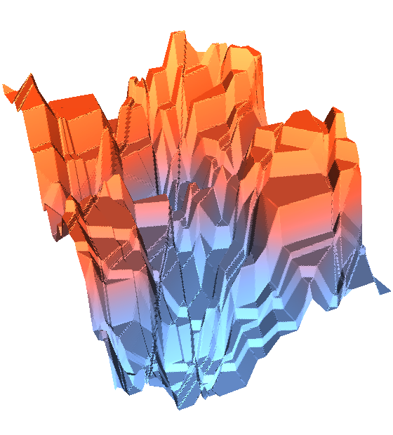
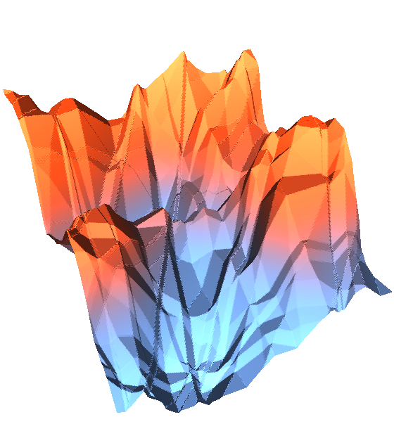
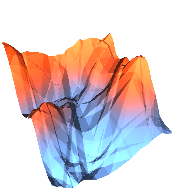
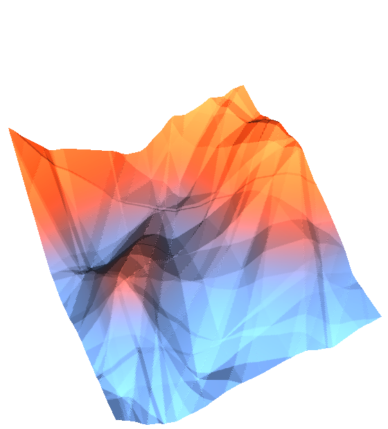
For the interested reader, we additionally present visualizations of smoothing effects introduced by different approaches for direct optimization of rank-based metrics. We display the behaviour of our approach using blackbox differentiation (Vlastelica et al. 2020), of FastAP (Cakir et al. 2019a), and of SoDeep (Engilberge et al. 2019).

In the following, we fix a 20-dimensional score vector $w\in\mathbb{R}^{20}$ and a loss function $L$ which is a (random but fixed) linear combination of the ranks of $w$ . We plot a (random but fixed) two-dimensional section of $\mathbb{R}^{20}$ of the loss landscape $L(w)$ . In Fig. 6(a) we see the true piecewise constant function. In Fig. 6(b), Fig. 6(c) and Fig. 6(d) the ranking is replaced by interpolated ranking (Vlastelica et al. 2020), FastAP soft-binning ranking (Cakir et al. 2019a) and by pretrained SoDeep LSTM (Engilberge et al. 2019), respectively. In Fig. 5(a) and Fig. 5(b) the evolution of the loss landscape with respect to parameters is displayed for the blackbox ranking and FastAP.

Acknowledgement

We thank the International Max Planck Research School for Intelligent Systems (IMPRS-IS) for supporting Marin Vlastelica and Claudio Michaelis. We acknowledge the support from the German Federal Ministry of Education and Research (BMBF) through the Tübingen AI Center (FKZ: 01IS18039B). Claudio Michaelis was supported by the Deutsche Forschungsgemeinschaft (DFG, German Research Foundation) via grant EC 479/1-1 and the Collaborative Research Center (Projektnummer 276693517 – SFB 1233: Robust Vision).

	$\displaystyle\sum_{i=1}^{n}W(r_{i})$	$\displaystyle=\sum_{k=1}^{\infty}W(k)\|\{i:r_{i}=k\}\|$
		$\displaystyle=\sum_{k=1}^{\infty}W(k)\bigl\|\{i:r_{i}\geq k\}\setminus\{i:r_{i}\geq k+1\}\bigr\|$
		$\displaystyle=\sum_{k=1}^{\infty}W(k)\|\{i:r_{i}\geq k\}\|$
		$\displaystyle\quad-\sum_{k=1}^{\infty}W(k-1)\|\{i:r_{i}\geq k\}\|$
		$\displaystyle=\sum_{k=1}^{\infty}\bigl(W(k)-W(k-1)\bigr)\|\{i:r_{i}\geq k\}\|$
		$\displaystyle=\sum_{k=1}^{\infty}w_{k}\|\{i:r_{i}\geq k\}\|$