A Newtonian analogue of Kerr black hole
Abstract
A 250-year old Newtonian problem, first studied by Euler, turns out to share a lot of similarities with the most extreme astrophysical relativistic object, the Kerr black hole. Although the framework behind the two fields is completely different, both problems are related to gravitational fields that have quite intriguing analogies with respect to orbital motions of a test-body in them. The fundamental reason responsible for their extraordinary similarity is the integrability of both problems, as well as their common multipolar structure. In this paper we demonstrate the existence of a multitude of either qualitative, and sometimes quantitative, similarities between the two problems. Based on this analogy, one could use the Newtonian problem to get insight in cases where the relativistic treatment of the field of a Kerr black hole becomes quite complicated.
1 Introduction
Struggling to solve the three-body problem in Newtonian gravity, Euler studied in 1760 an easier version of the general problem: the problem of motion of a particle in the gravitational field of two fixed centers with masses , at a distance apart from each other [1]. This problem, as it was much later shown by Whittaker [2], is characterized by such an internal dynamical symmetry that leads to a new integral of motion (according to Noether’s theorem for mechanical particle systems), rendering this particular mechanical problem fully integrable.
On the other hand Kerr black holes, that were first described and studied by Kerr [3] as an exact solution of the vaccuum equations of Einstein, proved to be the simplest macroscopic objects that Nature herself can create. They are fully described by only two parameters (the mass and the spin of the black hole, if we assume that the net electric charge of astrophysical objects is negligible according to astrophysical consensus); this is actually the physical context of the no-hair theorem [4]. During the golden era of general relativity (1970-1980) the physical characteristics of Kerr black holes, including perturbations of this metric, were studied extensively [5], and there is still an ongoing research on the subject in the framework of gravitational waves emitted from compact binaries [6], that is binaries consisting of neutron stars and/or black holes.
At least for binaries consisting of a massive rotating black hole and a neutron star, or a less massive black hole (known as extreme mass-ratio inspirals: EMRIs), could be studied perturbatively by considering geodesic orbits of the less massive counterpart in the gravitational field of a Kerr black hole [7]. The geodesic orbits around a Kerr black hole are described by an integrable system of differential equations (exactly as with the Newtonian gravitational field of the Euler problem), due to a Killing tensor field of the particular space-time that leads to a new integral of motion, the so called Carter constant [8, 9].
One might think that the similarity between the Euler problem and the Kerr metric ends exactly at this point, since the two gravitational fields do not look very similar from a physical point of view: Apart of the fundamental differences between the two corresponding physical frameworks (relativistic versus Newtonian gravity), the Kerr black hole describes an oblate gravitational field (due to its spin related to its axis of symmetry) of pure vaccuum, while the Euler problem is by construction ‘prolate’ in the sense that the mass of the system is distributed along its symmetry axis. However by introducing a purely imaginary distance –instead of a real one– between the two masses of the Euler problem [10], the corresponding gravitational potential remains real (the only necessary additional condition to obtain a real potential then is that the two masses are equal), while the global multipolar structure of its potential field becomes oblate; thus it becomes analogous to the Kerr gravitational field. Moreover, as Will [11] has shown, the only axisymmetrical and reflection symmetric Newtonian gravitational potential that leads to a third integral of motion that is quadratic in momenta (like the Carter constant) is the one that follows the same relation between successive multipole mass-moments with that of Kerr. Oddly enough, the Newtonian multipole mass-moments of the Euler problem with an imaginary distance are exactly the same with the Geroch-Hansen relativistic multipole mass-moments of the Kerr metric itself (the prolate version of the Euler field has the same ratio of moments but not the same moments). This very similarity between the two problems is fundamental for all the similarities of the orbital characteristics arising in both gravitational fields.
In this paper we have studied thoroughly the fundamental frequencies of the Eulerian orbits and have found numerous analogies with the frequencies of bound orbits in Kerr. Apart of the similarities in the expressions for the frequencies themselves, both problems have ISCOs. Moreover, one could find pairs of orbits –in both problems– that are characterized by exactly the same triplet of frequencies.
Stimulated by all these aforementioned analogies between the two problems, we have performed an extensive comparison of properties between the two problems and we found some new intricate similarities, that further persuaded us that the two problems could be considered quite faithful analogues of each other in Newtonian and relativistic frameworks, respectively. We believe that one could use this analogy to gain deeper insight into each one of them by studying its twin counterpart. As an example we have applied this analogy to clarify and explain the rather subtle argument of Kennefick and Ori [12] according to which the “circular” geodesic orbits in a Kerr background remain circular under their adiabatic evolution due to gravitational radiation. Not only the corresponding orbits in the Euler problem have analogous characteristics (they sweep over a surface of constant spheroidal radius that evolves adiabatically under a weak dissipative force), but the formulation of the Newtonian problem itself allows for a much more transluscent explanation than the one used by Kennefick and Ori for first time. The Newtonian variation of this proposition helps to better understand the foundations of that old but quite strong argument, and to explore it quantitatively in further detail.
Furthermore, the integrability of Kerr metric has been used in [13] to show that a hypothetical non-Kerr object could in principle be recognizable by its characteristic gravitational wave signal, due to its non-integrable character. During the crossing of an orbit in phase space through a Birkhoff island (the existence of which is a direct theoretical consequence of a slightly perturbed integrable system according to KAM theorem [14] and Poincaré-Birkhoff theorem [15]), the ratio of the corresponding frequencies in the signal spectrum should remain locked to a constant rational value for a while; this is the plateau effect which was analyzed in [13]. The initial computation of the relevant delay time was based on the average energy loss and average angular momentum loss as computed for a generic orbit in Kerr, suitably adjusted to account for the deviated lower multipole moments of the new space-time compared to the corresponding Kerr metric. In a foregoing paper, we plan to use the analogy between the Newtonian and the relativistic problem to check if this time interval could be systematically different if the evolution is computed by means of the instantaneous self-force acting on the particle, instead of being based on averaging formulae. The Newtonian problem could be easily perturbed to construct a slightly non-integrable system as a toy-model for a perturbed Kerr black hole.
The rest of the article is organized as follows: In Section 2 an overall description of the Euler problem is given, along with its oblate variant with an imaginary, instead of a real, distance. General characteristics of the orbits in the oblate Euler gravitational field is presented in Section 3. In Section 4 a list of the properties of the Euler problem, that are similar to the properties of Kerr metric, that are known up to now, are presented. In Section 5, an extensive list of new properties that reveal the close analogy between the two problems is presented. Finally, in Section 6, the argument of Kennefick and Ori from the perspective of the Euler problem is reformulated and explained. Furthermore, a quantitative result with respect to the evolution of the eccentricity of an orbit when the resonance condition is met –which actually could happen in ‘circular’ orbits in the Euler problem– is constructed. In Section 7 we summarize our findings, and suggest new problems that the similarity between Kerr and Euler field could further be used.
2 The Euler problem
2.1 The original problem
The gravitational field of two point-like (or spherically distributed) masses located at fixed positions in an inertial (in the Newtonian sense) frame of reference constitute the basis of the Euler problem, also known as the ‘two-centre problem’. Euler first studied the orbit of a test particle in such a gravitational field as an attempt to obtain analytical solutions in special cases of the general three-body problem (the motion of three particles of arbitrary masses under their mutual gravitational attraction). The gravitational potential of such a system is
| (1) |
where is the gravitational constant, are the two point-like masses and are the distances of the point, where the potential is computed, from the two fixed masses. If we use a coordinate system such that the two masses lie on the -axis at equal distance from the origin, then the gravitational field assumes the following form
| (2) |
This potential is obviously conservative and axially symmetric; consequently a test body orbiting this gravitational field will be described by a constant energy and a constant -component of angular momentum. The potential is not reflection-symmetric about the plane, except when the two masses are equal. However, whatever the masses are, the problem is characterized by a hidden dynamical symmetry that leads to an unexpected new integral of motion, quadratic in momenta. This integral of motion –initially we shall call it ‘Euler’s third integral’– is derived by applying the Hamilton-Jacobi method when we perform separation of variables in a suitable coordinate system [16]. Although, this 3rd integral of motion is known for more than a century, quite recently, Lynden-Bell [17], trying to explain its physical meaning, offered a simple and straightforward constructive method to build it. He proved that its kinetic part is the scalar product of the angular momenta about the two centers of mass and defined it as:
| (3) |
where is the particle’s velocity, are the vectors from either gravitating mass to the test particle, while are the unit vectors along the directions of , respectively. does not depend on the mass of the test particle orbiting the corresponding field. The existence of three independent integrals of motion, render the motion in such a field describable by an integrable set of equations. Only a few known physics problems are exactly integrable, and all of them are characterized by special common properties (for example the motion in phase space lies on a 3-torus and each such torus is characterized by a triplet of fundamental frequencies).
A more appropriate coordinate system to study the motion in the Euler gravitational field is that of prolate spheroidal coordinates, where one of the two coordinates, , is the sum of the distances from the two masses compared to the distance between the masses (this is the analogue of the radius of spherical coordinates, but endowed with an intrinsic length scale), while the other one, , is the difference of the two distances divided again by the distance between the two fixed masses (this is the analogue of the cosine of the polar angle in spherical coordinates). The third coordinate is the usual azimuthal angle of spherical, or cylindrical coordinates. Thus
| (4) | |||||
| (5) |
where , are the usual cylindrical coordinates. The spheroidal coordinates take values within the intervals: and . The inverse coordinate transformation yields
| (6) | |||||
| (7) |
In terms of spheroidal coordinates the Euler potential assumes the following form
| (8) |
The Lagrangian (per unit test-mass) of the Euler problem in spheroidal coordinates is then:
| (9) |
The corresponding canonical momenta in these coordinates are
| (10) | |||||
| (11) | |||||
| (12) |
and the Hamiltonian (per unit test-mass) assumes the following form
| (13) | |||||
According to Landau’s analysis [16] which is based on constructing the most general separable potential in such coordinates (called elliptical in Landau’s textbook), the separability of the particular problem arises from the very fact that the numerator in equation (8) is a linear superposition of a function of alone and a function of alone. The integrability of this potential then arises as a direct consequence of the separability of Hamilton-Jacobi equation. The third conserved quantity, in [16], besides the energy and the -angular momentum , gets the following form in spheroidal coordinates:
| (14) | |||||
| (15) |
The two alternative expressions for in Eqs. (14,15) are pure functions of and , or and , respectively, clearly demonstrating the separability of the problem. The constant is related with the expression for of Eq. (3) by , as one can verify by combining both expressions for (Eqs. (14, 15)), expressed in cylindrical coordinates and performing a lengthy, but straightforward, computation.
2.2 The oblate version of the Euler problem
As mentioned in Section 1, the gravitational field of the Euler problem describes, by construction, a prolate distribution of mass as a source (this will become more obvious later on, in Sec. 4.2, when we will present the multipolar structure of the Newtonian problem). Therefore it does not resemble the gravitational field of a Kerr black hole, which is obviously oblate (its quadrupole moment is negative). However, it is easy to transform the original Euler problem into an oblate field by simply rotating into a complex plane by . Then will transform into a purely imaginary distance, but the gravitational field will still be real, in the symmetric case where . Only then the gravitational potential of each mass is given by the complex conjugate function of the potential of the other mass. In order to avoid confusion we will keep considering the parameter real and simply replace by in the potential. The corresponding gravitational field –henceforth called the oblate Euler field– assumes the following form:
| (16) |
where by we mean . The latter vector product is a complex number and in order to keep the square root single-valued we should adopt a branch cut. We have chosen the negative real axis of the vector product as the branch-cut of our potential function. After some algebra the new potential (from now on we will use only this potential, so we will simply write it ) takes the following form in usual spherical coordinates:
| (17) |
where
| (18) | |||||
Although it is not obvious at this point that the new potential describes an actually oblate field, its true character will be unequivocally revealed in Section 4.2, where its multipole moments are written.
It should be noted that the new field is defined everywhere since , except of along the equatorial circle where the potential becomes indeterminate, since then . Also, on the equatorial disk the potential vanishes. The oblate Euler field is reflection symmetric, as the original prolate Euler field when the masses of its two gravitational centers are equal.
A more appropriate coordinate system to study the motion in this oblate field is that of oblate spheroidal coordinates, , which are defined as:
| (19) | |||||
| (20) | |||||
| (21) |
where , and . The surfaces of constant -coordinate are oblate ellipsoids of revolution with focal circle , while the surfaces of constant -coordinate are one-sheet half hyperboloids of revolution sharing the same focal circle with the above ellipsoids.
In terms of oblate spheroidal coordinates the Euler potential assumes the following simple form
| (22) |
The Lagrangian (per unit test-particle mass) of the oblate Euler potential becomes:
| (23) | |||||
while the corresponding Hamiltonian is
| (24) | |||||
with the canonical momenta defined as:
| (25) | |||||
| (26) | |||||
| (27) |
Repeating Landau’s argument [16], for the oblate field now, the very fact that the numerator in Eq. (22) is again a linear superposition of a function of and a function of (no presence of function here) lies behind the separability of the given problem, and consequently, the integrability of this particular potential. The third conserved quantity, , besides the energy and the -angular momentum , takes the following form:
| (28) | |||||
| (29) |
Once again, the separability of the problem is clearly manifested in these two expressions since the 4D phase space of breaks in two independent 2D phase spaces and , and the motion evolves along a closed line in each of these two phase planes.
3 The orbital characteristics in oblate Euler
The gravitational potential of the Euler problem (henceforth we will only deal with the oblate version of the Euler problem and we will omit any specific notation mark) describes a conservative axisymmetric field that admits a constant of motion, as we have mentioned earlier, that is quadratic with respect to momenta. This new constant could be considered as an analogue of the square of angular momentum of central fields. The new field is by construction not central though, but its dynamical structure is such that it renders the problem integrable. Furthermore, the choice of imaginary distance between the two masses renders the field oblate with respect to its dynamics, instead of prolate. This very fact make it more physical with respect to qualitative resemblance with spinning astrophysical objects.
The Kerr metric is a relativistic object of extreme astrophysical interest, which shares a lot of general properties with the Euler field as it will be shown in the following Sections of the article. Both gravitational fields are (i) integrable (with respect to the description of geodesic orbits of test particles orbiting around them), characterized by three, similar in context, constants of motion, (ii) have similar multipolar characteristics, and (iii) are fully described by only two physical parameters, their total mass and the spin parameter (for the Kerr) or the imaginary part of the distance between the two masses (for the Euler).
In the following section we will further study the orbital characteristics of the Euler problem in order to demonstrate the extent of similarity between the two fields.
3.1 Equations of motion
In order to compare the equations of motion in the Euler potential with those of Kerr we define new coordinates:
| (30) | |||||
| (31) |
The new coordinates play the role of the radial and the longitudinal Boyer-Lindquist (BL) coordinates of Kerr space-time, respectively. Although equivalent to the oblate spheroidal coordinates , the new coordinates are better suited to reveal the analogies with the corresponding orbits of Kerr metric. The 3rd coordinate, , is the usual azimuthal angle that is common in both problems. The comparison will be further simplified by adopting geometrized units () in the Newtonian field as well.
The Euler potential in these new coordinates is given by:
| (32) |
while the corresponding Hamiltonian (24) yields the following form:
| (33) |
where , while , , are the canonical momenta with respect to , respectively. The momenta and are related with the momenta and (c.f., Eqs. (25, 26)), respectively, through the following relationships: and . Since coordinate is missing from the Hamiltonian, is conserved, and henceforth we will write it, instead, .
Applying the Hamilton-Jacobi method in the above Hamiltonian (33), we obtain the following separated equations of motion for a test particle:
| (34) | |||||
| (35) | |||||
| (36) |
The radial potential and the longitudinal potential introduced in Eqs. (34, 35) are given by:
| (37) | ||||
| (38) |
where is the constant value of the Hamiltonian, is the conserved -component of its angular momentum and is a third integral of motion that naturally emerges from the above separation of variables, while is the Newtonian time parameter. In the next section 3.2, we define all these constants of motion in detail.
At this point, it should be noted that exactly the same equations of motion, but with slightly different potentials , show up in the description of the geodesics in Kerr metric. However in Kerr case the proper time , instead of the coordinate time , is the evolution parameter of the spatial BL coordinates .
The Eulerian orbits are performing a radial oscillation and a precession while they revolve around the axis of symmetry. The characteristics of are responsible for the radial oscillation, while those of are responsible for the oscillation of the test particle about the equatorial plane.
3.2 Bound orbits
As demonstrated in the previous section (c.f. Section 3.1), the Euler potential admits three constants of motion, which in terms of coordinates and momenta are given by the following expressions:
| (39) | |||||
| (40) | |||||
| (41) | |||||
| (42) |
The third integral of motion , written in two alternative forms in Eqs. (41, 42), one with respect to , and one with respect to , is related to Lynden-Bell’s , and Landau’s , through the relation:
| (43) |
We have decided to use , instead of and , as the third integral of motion, because this form of could be considered as the Newtonian analogue of Kerr’s Carter constant, as it will be shown later.
The two potentials , presented in the previous section, share a lot of similarities with the corresponding potentials of Kerr. More specifically, the later one, , yields exactly the same form as of Kerr, if we simply replace by (see Section 5.2), while is of order four, like that of Kerr, and most of the polynomial coefficients coincide with those of Kerr, if the previous reparametrization of is imposed here as well. Especially the fact that is a quartic polynomial, leads to the possibility of two families of bound orbits: (a) one with lower radii: , coexisting with another one with , where are real roots of the polynomial , and (b) one with only a single range of radii , while the other set of roots of are then complex conjugate to each other. We will consider bound orbits that correspond to the farthest family, if two of those exist. The reason is the following: the bound geodesic orbits in Kerr are either those that remain at the exterior of the event horizon, or plunging orbits that eventually cross the black hole horizon. The former ones are the ones at higher values of radii far from the horizon.
The family of orbits in Euler corresponding to lower radii, when both families are present, will be considered ‘plunging orbits’ at close analogy to those of Kerr. The second type (b) of bound orbits in Euler, with a single range of allowed radii, could either describe a normal bound orbit (without any plunging pair), or an effectively ‘plunging orbit’ in the sense that the two distinct regions of bound orbits of the first type have merged into a single region through a potential neck that will eventually drive an orbit to a plunging one (see Figure 1(d)). The latter type of orbits will not be treated as simple eccentric orbits with a periastron and an apastron, since it does not seem natural to describe them as orbits with a specific semi-latus rectum and eccentricity. In our description of possible bound orbits in the Euler potential we will not consider such type of orbits.

Next we will follow the same procedure one uses to study the bound orbits of Kerr: we will parametrize the roots of as follows
| (44) |
assuming they correspond to the outer bound orbit (if there exists an inner region as well) described by the dimensional semi-latus rectum and the eccentricity . The rest of the roots of , (either real or complex) could then be computed as functions of the orbital parameters and the inclination angle of the orbit (where is the lowest polar angle of the orbit). The set of the three orbital parameters could be used not only to compute the roots of , but from them one could compute the constants of motion, as well (see Appendix B).
Meanwhile, the oscillation of parameter around the equatorial plane () is governed by potential as mentioned previously. The roots of are two real supplementary angles which correspond to the turning points of orbital-plane oscillation and two complex imaginary angles. The roots of are described in Appendix B.
As mentioned above, the constants of motion , and are directly related to the orbital parameters , but they are not as easy to handle as the orbital parameters. Although analytic expressions for as functions of could be written they are quite involved. Furthermore, by fixing the constants of motion, one could get a set of two bound orbits, an interior one and an exterior one, but then one has to chose to which one a semi-latus rectum and an eccentricity should be assigned. In contrast, as long as one gets restricted in a meaningful space of the orbit is unambiguously determined. This is actually the reason we have chosen to use the orbital parameters in order to parametrize the orbits.
3.3 The separatrix
In the 3-dimensional space of orbital parameters there is a special surface, which corresponds to a pair of orbits: one normal bound orbit and a “plunging” one that share a common turning point, that is (c.f. Figure 1(b)). This surface is the separatrix. The normal bound orbits of the separatrix are actually marginally stable orbits. Eventually these orbits will evolve into circular orbits with radius . One expects that a slight variation of the physical parameters of the orbit (), due to any kind of dissipative self-force acting on the test particle, could cause the two families of orbits to either communicate (by transforming the normal bound orbits into “effectively plunging” orbits), or move the two types of orbits further apart. Actually, the neighborhood of mostly the whole surface of the separatrix corresponds to the latter case. Both sides of the surface (but close to it) describe pairs of two distinct separated families of orbits, one above the separatrix with orbital parameters () and one below the separatrix with orbital parameters () with , such that both are described by the same potential with the same contants of motion. The one with is actually the plunging one, dual to the normal one with ; therefore we will deal only with orbits located ‘above’ the separatrix.
Near the edge of the separatrix (corresponding to the most inclined orbits of the separatrix) there are orbits that are effectively plunging ones like that of Figure 1(d) and as we mentioned earlier, we will not study such orbits.
The separatrix could be described as follows: For a given pair of eccentricity, , and inclination, , there is a specific semi-latus rectum that brings the two types of orbits (the exterior normal orbit and the interior plunging one) in touch. For equatorial orbits, , one could easily obtain an analytic expression for (by setting and, , while in Eq. (37), and write it in terms of the roots of the polynomial). For generic inclined orbits though it is a bit more difficult to obtain an analytic expression for as a function of , and . We found useful to introduce an additional parameter , in order to write an analytic expression for and then plot the surface in parametric form, since itself could be directly expressed as a function of as well. In Figure 2 the separatrix surface has been plotted for a specific value of , namely . All the above analytic derivations are thoroughly analyzed in Appendix C.

The separatrix extends from (equatorial orbits) to a minimum value of that depends –not very sensitively– on the eccentricity, . More specifically , for , and it increases monotonically to , for . The overall shape of the surface is the same for any value of , while the value of scales linearly with , assuming its highest value, , for , (which corresponds to ). Beyond the lower values there is no separatrix; that is, there are no more four real roots of . A complex pair of roots arise then.
Now let us study in further detail the region of parameter space outside the separatrix. On the region just above (but not far from) the separatrix () the two types of orbits (stable bound and “plunging”) get separated (). As we mentioned previously, below the separatrix the order of roots is alternated ; therefore there is lack of physical description of such orbits based on the assumption that the order of roots is and the bound orbit oscillates radially between and . Each such point (), located below the separatrix, has its dual above the separatrix with a different set –but with the same inclination– such that , therefore both these points correspond to a normal bound orbit that oscillates radially between and . Far from the separatrix surface (either below or above it) the potential looses a pair of real roots, thus, then, there is only a single bound orbit corresponding to it. Finally in a rather narrow space around the boundary of the separatrix, corresponding to the lower possible value of , there is a bizarre type of bound orbits (the effectively plunging orbits) arising from the merging of a stable bound orbit with a “plunging” one. The potential in such cases has a local minimum between its two real roots (see Figure 1(d)). Although we will not deal with such orbits, there is a finite lower and a finite higher allowed radius for those as well, so one could still use the analytic expressions for the frequency of the radial oscillations, which we will introduce later on.
Especially the boundary of the separatrix with corresponds to margin-ally stable “spherical” orbits (or, as they are usually called in Kerr metric, “circular” orbits). It should be noted that the boundary of the separatrix corresponding to equatorial orbits () is given by a monotonically increasing function , like in Kerr, but it has the opposite sign of curvature. In both problems the “corner” of the separatrix at and (equatorial orbit), which corresponds to the ISCO, represents the lowest semi-latus rectum among all marginally stable spherical orbits.
4 Known analogies
In this section we present a list of the analogies between the two problems, the Euler and Kerr, that have already been shown in the literature by various authors in the past. Most of these analogies were presented in different context from the one followed in this article and in most of them there is no clear connection between Kerr and oblate Euler field.
4.1 Basic common characteristics and fundamental differences
During the golden era of black holes, when extensive mathematical studies had been performed, Israel [18] ended up in the oblate Euler field (without recognizing it as such) as the Newtonian analogue of Kerr metric by means of the right source distribution of the gravitational field. Actually the analogy between the two fields had been revealed even earlier by Keres [19], but it was mainly focused on finding similar properties related to the ring singularity of the then recently discovered Kerr metric and the corresponding avoidance of the ring singularity by geodesics. There was no demonstration of any connection between the two gravitational fields with respect to the orbital characteristics in them.
The present study attempts to extend this old found similarity between the two fields, mostly in the direction of astrophysically oriented issues, like geodesic orbits at the exterior of a Kerr black hole and their properties.
It should be pointed out though, that there are fundamental differences between the two fields. At first glance there is a dimensional difference of the parameter showing up in the two fields. For the Kerr metric the parameter is related to the spin of the Kerr black hole, thus it has dimensions of length times velocity (it is actually the ratio of the angular momentum of the black hole to its mass ). In Euler’s oblate problem the parameter is simply a length. Although in geometrized units, both parameters have length dimensions, (or equivalently mass dimensions) the two ’s still have completely different physical origin. Despite that, this parameter, (or its dimensionless counterpart in geometrized units where ), seems to play the same role as an adjusting parameter of the two fields and their correspondence.
However there is an essential difference in the use of in the two problems: in Euler’s problem could assume any value, while in Kerr cannot exceed the value of 1 (hyperextreme Kerr). However the restriction for the in Kerr is mainly related to the existence of a horizon in Kerr, which has no analogue in Newtonian gravity in the first place. Here we will restrict our study of the Euler field in the range .
Another technical difference arising between the two problems is the asymmetry of Kerr metric under the transformation (one should amend such a transformation with , as well, to produce an isometry, but then the Kerr spin parameter will change its sign). By contrast, Euler’s problem (as any other type of axisymmetric Newtonian potential) is completely symmetric under such a transformation . Consequently, the dragging of frames arising in stationary axisymmetric relativistic configurations, like in Kerr, does not have its analogue in Newtonian gravity. Therefore we shall be very careful when we compare the quantitative characteristics of phenomena that are sensitive to the sense of rotation in Kerr, with the corresponding ones in Euler’s field.
4.2 Multipolar structure
More recently, Will [11] showed that the Newtonian axisymmetric gravitational field that is characterized by a third conserved quantity analogous to the Carter constant of a Kerr space-time (that is quadratic in momenta), leading, consequently, to an integrable Newtonian potential, should have a multipolar exapnsion that follows exactly the same relation as the mass multiple moments of the Kerr metric itself, that is
| (45) |
while its odd- mass moments vanish (as one would expect for a reflection symmetric gravitational field). It should be noted that this multipolar structure describes exactly the Euler’s field (both the oblate and the prolate one) with equal masses. More specifically, if it corresponds to the original Euler’s field (the prolate one), while if it corresponds to the oblate version of the Euler’s field. Naturally, the case is the monopole, spherically symmetric, Keplerian field, for which the corresponding third integral of motion is simply the square of the total angular momentum of an orbiting test particle, instead of the constant , discussed in the previous section.
Of course a Newtonian stationary and axisymmetric potential cannot reproduce any effect like the dragging of frames of the corresponding relativistic field, and thus there are no current-mass multipole moments like that of Kerr. This is one of the basic differences between the two fields, and that renders the comparison between the corresponding orbits in the two fields more subtle. We will further discuss this subtlety in Section 5.3.
Later on Markakis [20] attempted to generalize Will’s result, looking for Newtonian gravitational fields that admit integrals of motion of higher order (in particular quartic with respect to momenta). His analysis yielded a null result. If the analogy between the Euler’s problem and the Kerr metric could be extended to problems with other type of non-Carter-like integrals of motion, the negative result of Markakis could be just a hint that probably there is no integrable vaccuum stationary and axisymmetric solution describing an isolated object other than the Kerr in General Relativity.
4.3 The separability of the wave equation
As it was shown in [21] the gravitational field of the Euler’s problem, not only leads to a lot of similarities in the characteristics of test-particle orbits with those of the gravitational field of Kerr, but the separablity arising in the equations that determine the orbits (for both problems), is also exhibited in the scalar wave equation in both gravitational fields. Therefore the Newtonian type of wave equation
| (46) |
where is a Newtonian potential, and is a constant with dimensions of frequency squared, becomes separable in spheroidal coordinates if the potential is that of the Euler’s problem. Moreover, the wave solutions of the oblate Euler’s problem can be written as a product of an angular part that has exactly the same form as the corresponding angular part of the scalar perturbations in Kerr, while the radial part has qualitatively very similar behavior, especially if , where is the corresponding frequency of the wave solution. To reveal this magnificent analogy one should consider the following correspondence:
| (47) | |||||
| (48) |
where (for more details about the definition of see [21]). The odd correspondence between and Boyer-Lindquist coordinate was chosen in order to transform the radial part of the wave equation into a form that is as close to that of Kerr as possible, and it is related to the fact that the radial coordinate in Kerr should not be interpreted as a spherical coordinate in flat space. For sufficiently large values of though, , as it can be easily shown.
Therefore, not only the two problems lead to separable wave equations, but the corresponding eigenfunctions, on which any wave perturbation can be decomposed, are quite similar. More specifically the angular eigenfunctions are exactly the same, while the radial ones, although not identical, they have the same behavior at large radii.
5 Revealing new analogies
We devote this section in constructing an extended list of new analogies that demonstrate the close analogy between the relativistic gravitational field of Kerr space-time and the Newtonian gravitational field of the oblate Euler’s problem.
5.1 Orbital precession
It is well known that a bound geodesic orbit around a Kerr metric, generally oscillates about the equatorial plane, while it revolves around the black hole. Thus an orbit with never crosses the symmetry axis; but it oscillates within a maximum angular amplitude about the equatorial plane. This angle is called the inclination of the orbit (see [5]), and it could be easily obtained by computing the extreme angles, , constraining the -oscillation. This is directly regulated by the value of Carter constant . Especially, for the orbit is strictly equatorial.
Since the connection between , and for the Euler’s problem (52) is exactly the same with that for Kerr (after adopting a redefinition of the constant , discussed in Section 3.2), the orbits of a test particle in the oblate Euler’s problem will have similar azimuthal properties with those of Kerr. As long as an Euler orbit is characterized by , its (related to the spheroidal coordinate ) oscillates back and forth around zero, while the corresponding extreme values of are symmetrical to each other, determining the inclination of the orbit. Again when the Carter constant of Euler vanishes, the orbit is equatorial.
Furthermore, in both problems, a bound orbit, while revolving around the axis of symmetry, and oscillating around the equatorial plane, it also moves radially in and out between two extremal radii (). If these two radii are equal then we get a “circular” (or as we call it here “spherical”) orbit. In the Kerr case circular orbits have been shown to be stable against gravitational wave perturbations. Later on, we will demonstrate that this is not generally true for bound orbits in Euler. Although this is a qualitative difference between Kerr and Euler, this particular difference between the two problems enhances the qualitative similarity between the two problems, since the resonance condition on which the whole argument about stability is based, can be used for both problems. It happens that in the Euler case there are physical parameters for which the resonance condition holds true; consequently the corresponding spherical orbits become unstable. In Kerr case there is no such resonance for any bound orbit; thus spherical orbits are stable. Section 6 is especially devoted to demonstrate how this difference arises when applying the same argument in the two qualitatively similar problems.
Finally we should add that for both problems, usually there is a pair of bound orbits, one of which corresponds to actually plunging orbits in Kerr case (since such an orbit is partly buried beneath the horizon of the black hole). In contrast the Euler problem is not endowed with any horizons, thus this family of orbits are still regular orbits with lower extremal radii () than the corresponding extrema () corresponding to its normal counterpart orbit. To keep a close correspondence with Kerr orbits though, we will baptize this new family of orbits “plunging orbits” as well, and we will not study them furthermore.
As mentioned before, it should also be pointed out here that there is another fundamental difference between the two problems. In Kerr space-time the prograde orbits (orbiting at the same sense as the spin of the black hole) and retrograde orbits (orbiting at the opposite sense) are distinct; they have different characteristics. This is due to the Lense-Thirring effect caused by the spin of Kerr metric, and it arises due to the nonvanishing current-mass moments of the corresponding metric. The current-mass moments, though, are not present in a static Newtonian gravitational field; therefore the prograde and retrograde orbits are completely equivalent in the sense that they become identical under the transformation . This qualitative difference between the two fields is emphasized in those cases where the description of a phenomenon encompasses linear functions of in the Kerr metric, while only the square of shows up in the corresponding description of the Euler problem. When some particular property of the Kerr field, that differentiates a prograde from a retrograde orbit, is compared to the corresponding one of the Euler field, naturally, disagreements will appear. We will handle this comparison with great care by considering an average of a carefully chosen pair of orbits (consisting of one prograde and one retrograde), both characterized by the same physically measurable quantity (see below at Section 5.3).
5.2 The Carter-like constant
The Carter constant is a conserved quantity along the geodesics in Kerr space-time. In Boyer-Lindquist coordinates, when expressed in terms of momenta, it takes the following form:
| (49) |
while, when expressed in terms of momenta, it takes a quite different form:
| (50) |
where . In the expressions above, , are the conserved energy () and the conserved -component of the angular momentum () of an orbiting test particle. Both momenta are proportional to the particle’s rest mass ; thus itself is proportional to . Equivalently, one could construct the reduced quantities , , , , , and rewrite the above expressions in terms of the corresponding reduced quantities, that are not related to the test particle, but only on the particular geodesic. For simplification we are going to use Eqs. (49, 50) themselves, without the tilde signs, but referring to the reduced quantities. This is equivalent to the quantities of a test particle with rest mass .
Earlier (in Section 3.2) we derived Euler’s third integral of motion (c.f. Eqs. (41, 42)). By rewriting the energy of the Euler field in terms of its relativistic analogue at the non-relativistic limit:
| (51) |
we get, after omitting the corresponding (K) marks, the following expressions for the Euler’s Carter constant:
| (52) |
in terms of , and after some term rearrangement:
| (53) |
in terms of . Although the second expression for could be written in a simpler form where the parameter shows up solely through (the terms linear in in Eq. (53) vanish if we expand it), we have chosen the above formulation in order to have a closer comparison with the corresponding expression for Kerr (see Eq. (50) above). Note that the first formula (52) has exactly the same form as the Carter constant of Kerr (49), while the second one (53), although quite similar (both are rational functions built from polynomials of the same order with respect to ), apparently it does not matches exactly the form of for Kerr. However, it should be noted that the presence of the mass of the source, , only at the last term of the expression (53) for Euler’s , although it seems to have no analogue term in the corresponding expression for in Kerr, this is misleading. The presence of in in Eq. (50) will show up exactly as when in the denominator of the first term is expanded at lowest order with respect to and assume that the particle moves at the weak gravitational field where . Of course the two problems are not identical to each other, and this is the best analogy between the two expressions we could achieve. At the weak field limit though the similarity is even better.
5.3 The ISCO
The usual gravitational field of a Newtonian monopole lacks the analogue of an innermost stable circular orbit (ISCO) which is present in the gravitational field of a Schwarzschild black hole. The reason is that the centrifugal potential in Newtonian gravitational fields acts always as a repulsive potential which, compared to a suitably soft gravitational field like that of a Newtonian monopole, it ensures that there is always a stable circular orbit at any radius. This could be considered as a clear difference between the relativistic (Kerr) and the Newtonian (Euler) gravitational field at the limit .
This fact is deceiving though. The Euler’s problem has also an ISCO for any non-vanishing value of . If one considers a circular orbit on the equatorial plane () of the Euler’s oblate field, then the corresponding effective potential in cylindrical coordinates is
| (54) |
where is the reduced -angular momentum of the test particle (or the angular momentum for a unit mass particle). In terms of the oblate spheroidal coordinates instead, the above potential assumes the following form:
| (55) |
By solving simultaneously the equations , corresponding to the presence of an ISCO, leads to . Thus the oblate Euler problem does have an ISCO, the actual radius of which in cylindrical coordinates is
| (56) |
or in spheroidal radius
| (57) |
Note that is not the real Euclidean distance from the origin to the test particle at ISCO (the Euclidean distance is ), but it is the analogue of the Boyer-Lindquist radius of Kerr, which we use extensively in our paper in order to draw a faithful comparison of Euler with Kerr.
Oddly enough, the existence of ISCO in the Euler problem is still present even in the limit ; the corresponding radius just tends to then. This is a new qualitative feature that the Newtonian monopole field () lacks, as mentioned previously. Therefore, the case (but ) could be considered as the analogue of a Schwarzschild black hole. Note, also, that contrary to oblate Euler problem, the original Euler problem (the prolate one) does not possess an ISCO. This is due to the fact that in the prolate Euler field the attraction from the two point sources, located along the -axis, is even softer than the Newtonian one from a single point source; therefore the repulsive centrifugal potential rules out the existence of an ISCO in this case.
The critical value of -angular momentum leading to the presence of ISCO in the oblate Euler field is
| (58) |
while the corresponding expression for the Kerr field is quite involved and difficult to compare with the above simple formula, since the expression of the -angular momentum for a prograde and a retrograde orbit as a function of is different, due to the Lense-Thirring effect.
Although the existence of an ISCO in the Newtonian problem is by itself a positive qualitative sign of the physical resemblance with the relativistic problem of a Kerr black hole, apparently it does not seem to share any quantitative similarity with the dependence of ISCO radius in Kerr with its spin parameter (see [22]):
| (59) |
where
| (60) |
and
| (61) |
with while the two signs correspond to prograde (upper sign) and retrograde (lower sign) orbits, respectively. As mentioned previously the ’s showing up in the expressions for the ISCO radius in the two problems have completely different physical origin: in Euler field it’s just a distance, while in Kerr field it is related to the angular momentum of the gravitational source itself; therefore apart of the existence of an ISCO radius in both problems, no qualitative similar behavior of with was anticipated. In Figure 3 the ISCO radii as a function of for both types of orbits in Kerr are plotted. The apparent non-linearity –especially for the prograde orbit–, in contrast to the linearity of the oblate Euler problem, is clear.

On the other hand the comparison between the two problems is not exactly fair from a physical point of view. The relativistic problem, although axisymmetric, strongly discriminates between the two opposite senses of rotation of an orbit (it is not symmetric under the transformation ), while the Newtonian one is absolutely symmetric under such a transformation. Thus two circular equatorial orbits in Kerr that rotate at opposite senses at the same radius are not equivalent. It should be more appropriate to compare two orbits (a prograde and a retrograde one) with opposite rotational frequencies, after taking into account the frame-dragging of space-time itself, as in the case for two oppositely directed circular orbits in Euler’s problem at the same radius. Of course such pairs of circular orbits in Kerr will not have the same radii; thus one should assign some kind of an average value of radius for such a pair of oppositely, equally rotating, orbits in Kerr. To compute the actual rotational frequencies in the Kerr metric, means that one should firstly subtract the rotational rate of space-time itself, that is the rotational rate of ZAMOs [23]. Then one should seek ISCO orbits with equal absolute values of rotational rates with respect to ZAMO observers, in order to nullify the relativistic effect of frame-dragging and put the oppositely directed orbits on equal footing. In order to accomplish such a comparison of ISCO radii between oblate Euler’s problem and Kerr, we followed the following process: (i) For the Kerr case, first we plotted at the radius of ISCO as a function of for both prograde and retrograde orbits (see Figure 4). It is clear that the retrograde orbits have monotonically decreasing rotation rate with , which qualitatively follows a similar behavior with the rotation rate of circular Keplerian orbits , while is increasing with .

Instead, the rotation rate of prograde orbits have completely different dependence on . These orbits lie so deep in the strong gravitational field of the black hole and the frame-dragging effect is then so dramatic (the region close to is actually buried inside the ergoregion which has no analogue in Newtonian gravity), that their behavior with respect to rotational frequency is completely different from those in the Newtonian problem. More specifically, there is no corresponding retrograde ISCO orbit that rotates at the same rate (relative to ZAMO observers) for almost any prograde ISCO orbit, except of the prograde ISCO orbits at large, but not extremal (), values. The range of ’s of prograde orbits with a corresponding dual retrograde orbit, sharing the same , is . On the other hand for any retrograde ISCO orbit (corresponding to any value of ) there is a corresponding prograde one (one with the same value of ). Therefore we could form pairs of retrograde-prograde orbits with the same physical rotation rate . On each such pair we assigned the of the retrograde one (since this is the one that has a counter-rotating dual with some value, for every value of ). (ii) Then we numerically computed the ’s for both orbits (the retrograde (R) corresponding to and the prograde (P) corresponding to , both characterized by the same ). (iii) For each such pair we computed the average value of ISCO radii, , according to the relation
| (62) |
that takes into account the two radii of the oppositely rotating orbits on equal footing. (iv) Finally we have plotted as a function of and the output was apparently almost linear (see Figure 5), like in the Euler case.

Although it might seem rather artificial the way the was defined, we believe there is actually no other way to define a radius of ISCO that treats both the retrograde and the prograde orbits on equal footing as it is always the case with axisymmetric Newtonian problems. The only alternative natural way we could think of in order to form pairs of equivalent oppositely directed orbits is by assuming orbits with equal absolute values of angular momenta, instead of orbital frequency. We tried that as well but there is no pair of retrograde-prograde orbits with the same value of . In contrast to , is a monotonic function of , for , where the sign of determines the rotational direction of the orbit. The deeper reason is that the frame-dragging effect is so enhanced for large values of that one needs extreme value of angular momentum to keep a circular orbit stable, when it lies deep in the gravitational potential.
For completeness, we should note that the above method to construct equivalent pairs of prograde and retrograde orbits, leads to a double solution only for the case of , since then there are two values for a prograde orbit with the same of a corresponding retrograde orbit; one of them being the zero spin case. For continuity reasons though, we have ignored the second root –that of zero spin.
As we mentioned earlier, the dependence of ISCO radius of the Euler’s problem on parameter, is linear (c.f. Eq. 57)). Amazingly, this is approximately the behavior of in Kerr case with respect to the spin parameter , when a retrograde and a prograde orbit are considered as a suitably equivalent pair. A last comment on this similarity is that quantitatively the approximate linear fashion of with in Kerr, although of the same order, it does not have the same slope with that of Euler, which is .
To further stress this peculiar equivalence of oppositely rotating orbits in Kerr, we have also plotted the square of the average value of ’s for each such pair of equally rotating orbits as a function of (see Figure 6). Apparently this plot is also almost linear as in the Euler case, according to Eq. (58). The corresponding slopes though are remarkably different.

5.4 The fundamental frequencies
The Euler potential is an integrable system with three independent and in involution integrals of motion. The conjugate momenta and (cf. Eqs. (42) and (41)) are functions only of , and , respectively. For bound orbits (see Section 3.2), the space of trajectories is a compact and connected manifold. According to Arnold’s theorem [10], the phase space is diffeomorphic to a three-torus. Since the problem is integrable, even though the coordinates are not really periodic, their oscillation (or libration for ) correspond to characteristic frequencies, the so called fundamental frequencies.
Consequently, we could define a set of symplectic coordinates, the corresponding action-angle variables , where the angle variables are periodic functions of time, and the action variable corresponds to a fixed vector. The three frequencies related to the periodicities of ’s are the fundamental frequencies that one obtains by Fourier analyzing the oscillating (or librating) time dependence of the coordinates and coordinates of a bound orbit.
The generating function of the canonical transformation is the Hamilton’s characteristic function , which is the solution of Hamilton-Jacobi equation :
| (63) |
where are the old coordinates and their conjugate momenta are defined as: , , and , (the corresponding potentials are given explicitly in Eqs. (37, 38)). The first integrals of motion are: . Due to the separability of the Hamilton-Jacobi equation its solution is of the form:
| (64) |
where:
| (65) | |||||
| (66) |
The action variables are defined as (see [10]):
| (67) |
where the integration is to be carried over a period of oscillation or rotation of .
The action variables are constants of motion, as they depend only on the first integrals . Inverting them we can express the integrals as functions of the action variables. In particular the Hamiltonian can be expressed as and it is cyclic with respect to . The generating function also can be expressed in terms of the coordinates and the action variables:
| (68) |
The transformation equations are:
| (69) | |||||
| (70) |
while the equations of motion in action-angle variables become:
| (71) | |||||
| (72) |
The corresponding angle variables are periodic and linear functions of time:
| (73) |
where and are constants and describe the fundamental frequencies of the orbit. In Appendix D we give analytic expressions of the above quantities, . Here we simply give the final expressions:
| (74) | ||||
| (75) | ||||
| (76) |
where , and are the complete elliptic integrals of the first, second and third kind, respectively [24]:
| (77) | ||||
| (78) | ||||
| (79) |
with (where are the two roots of , with ) and . The integrals , and are related with the radial motion and are defined as:
| (80) | ||||
| (81) | ||||
| (82) |
with being the radial potential introduced in Eq. (37).
Although the orbit is not periodic, there are specific cases, where the motion is clearly periodic. A resonant orbit, where the ratio is a ratio of integers, is a more involved case of a purely periodic orbit since then an integer number of oscillations of , and (not necessarily the same numbers) are repeated in a finite time period.
For comparison the fundamental frequencies of a bound orbit in Kerr space-time have been derived by Schmidt [25] and they are given by exactly the same expressions with that of Euler (74)-(76), with and the two roots of the Kerr polar potential (which is the same with the polar potential of Euler). The radial integrals for Kerr though are given by (see [25]):
where the corresponding potential is
If we rewrite the Newtonian energy of the potential of Eq. (37) as previously: that is by adopting the reparametrization , we obtain a form of the radial potential of Euler which differs from that of Kerr only on the linear term. Therefore whatever differences in frequencies between the Kerr and the Euler field, arise from this difference in and the different expression of the integral.
5.5 Pairs of isofrequencies
Warburton et al [27] have shown that Kerr black holes (Schwarzschild black holes included) have an interesting property: there is no one-to-one correspondence between orbital characteristics and fundamental frequencies, that is, there are pairs of distinct bound geodesic orbits lying in the strong field region, that are characterized by exactly the same triplets of frequencies (radial, azimuthal, and longitudinal). Motivated by the fact that the oblate Euler field has an ISCO, like the gravitational field of a Kerr black hole, we looked for pairs of distinct, potentially synchronized, orbits in the Euler field as well.
Following the procedure of [27], we first searched for pairs of equatorial orbits with equal doublets of frequencies. While the third frequency, , could also be computed for such orbits, it does not show up in the orbital motion, since the orbit is purely equatorial. In order to seek such double solutions in the frequency space, we have plotted the contours of in the plane. Actually the very shape of the boundary of all possible equatorial orbits in the parameter space mentioned above, namely the contour-curve corresponding to , is sufficient to ensure the existence of pairs of orbits with the same set of frequencies. The boundary consists of orbits: (i) with infinite semi-latus rectum , corresponding to , but with various eccentricities (infinitely distant bound orbits), (ii) with eccentricity (marginally closed orbits), corresponding to a range of frequencies depending on the semi-latus rectum, and (iii) the separatrix, that is, orbits corresponding to a potential with a double root (and ), such that the orbit spends infinite time to complete an -oscillation between and . The ISCO is simply the endpoint of the separatrix at , corresponding to a marginally stable circular orbit, due to a suitable tuning of the polynomial expression for the potential , to obtain a triple root, (see Section 5.3). Along the separatrix of equatorial orbits, is given by the simple expression
| (83) |
where , since the particle will eventually end up to radius . Following Eq. (144) of Appendix C, the -frequency of such orbits could be expressed as:
| (84) |
The separatrix has positive slope, . Consequently, the boundary of the contour plot, , forms an inverted trapezoid (as in Kerr) in the parameter space . Due to continuity of the function for equatorial orbits, this shape is conclusive for the existence of isofrequency pairs of orbits (see Figure 7), as pointed out also in the case of Kerr [27].

In Appendix C we give analytic formulae for the constants of motion at the separatrix and from them one could compute, based on the expressions of Appendix D, the fundamental frequencies for these peculiar marginally whirl-zooming equatorial orbits. Apart of the separatrix, the bound equatorial orbits exhibit the following characteristics: (i) There is a maximum value of , which corresponds to a circular orbit (), marked as ‘’ in the contour plot of , Figure 7. The analytic expression for at zero eccentricity is simply
| (85) |
Thus the maximum value of is , for and . (ii) There is a line of non-circular orbits, called ‘COD’ curve (circular orbit duals) in [27], that have the same frequency set, , with a single corresponding circular orbit. The range of ’s that the COD curve spans is , corresponding to specific circular orbits marked as ‘’, ‘’ in the parameter space, respectively. The ‘’ circular orbit is simply the ISCO orbit, representing the maximum value of a circular orbit (with ), the dual of which is a non-circular orbit with (the upper end-point of the green dashed curve of Figure 7). On the other hand ‘’ is the circular equatorial orbit with a non-circular dual which has the lowest and the highest that such an orbit could yield. The ‘’ circular orbit is actually a singular case since the twin pair of the corresponding circular orbit is exactly the same orbit, representing now a marginally non-circular orbit. On the left side of the COD curve one could find all possible iso-frequency pairs. (iii) Finally, there is another special curve representing all iso-frequency pairs with marginally equal orbital parameters. Along this curve the Jacobian of the transformation between the frequency parameter space and the orbital parameter space vanishes, which means that the transformation is singular: each point along this line corresponds to a double root of the system of equations
| (86) |
This curve joins the points of the iso- contour lines that represent the extremum values of for each . This singular curve spans all eccentricities from marginal bound orbits () to circular orbits () meeting the COD line at point ‘’. As mentioned above, point ‘’ represents a singular circular orbit which is the dual of itself. The other end-point of the singular curve (the left-most corner of the plot in Figure 7) corresponds to the highest possible value for any bound orbit, and it is denoted as ‘’ in the contour plot. Since this orbit is an orbit at the separatrix, its semi-latus rectum is (this is what one yields from the parametric Eq. (144) when the values and are imposed), while its corresponding frequency is .
In order to plot the singular curve we have to solve the equation
| (87) |
The Jacobian of the transformation was computed numerically for arbitrary eccentricities. However the base of this line, ‘’, corresponding to zero eccentricity was derived analytically since then the complicated functions , and , could be written as simple analytical expressions, when expanded as Taylor series around . Both frequencies yield the form . Therefore the Jacobian of the transformation is linear with respect to near . This explains why all iso- contours are intersecting the -axis at right angles; that is, a slight eccentricity does not alter both frequencies of the corresponding circular orbits at order . More specifically, the Jacobian determinant of the transformation near yields the following form
| (88) |
Thus the starting point ‘’ of the COD line (at ), which coincides with the starting point of the singular line, is given by the solution of the algebraic equation , which is
(the second solution is lower than the ISCO radius so it has been omitted; this corresponds to the semi-latus rectum of the dual plunging orbit that lies beyond the separatrix). Finally, from the semi-latus rectum one can compute the two frequencies , and . The numerical values of these frequencies are and .
| 0.189 | 0.135 | 0 | 0 | |
| 0.299 | 0.401 | 0.439 | 1 | |
| 2.236 | 1.839 | 1.732 | 2 | |
| 0 | 0 | 0 | 1 |
| 0.0790569 | ||
| 0.453379 | ||
| 0.5370696 | 0.2 | |
| 1.94569 | 1.83337 | |

In Table 1 we summarize the above results by presenting a complete list of the values of all characteristic frequencies discussed in the previous paragraph (all are simply multiples of the dimensional quantity ), as well as the corresponding semi-latera recta, , of these orbits. It should be emphasized that not only the characteristic frequencies, but the frequencies of any bound orbit in the Euler field, are all scaled with , independently of and ; they depend only on the characteristic orbital parameters and . Therefore the contour plot of Figure 7 does not represent a specific value, as in the Kerr case. In contrast the exact form of the contour curves in Kerr does depend on , due mainly to the dragging of frames in the corresponding relativistic problem. The shape of the -contour lines on the left of the COD line ensures that one could find pairs of equatorial orbits with different orbital parameters but with the same set of frequencies. Two such orbits have been plotted in Figure 8 and have been marked (as and ) on the contour plot of Figure 7.
There is also one more similarity connected with the orbital frequencies. The Schwarzschild gravitational field is a specific case of a Kerr metric, the orbits of which are not closed due to different values of and . Also the Euler field, even when , has orbits that are not closed, as well, (the ratio is not identically equal to unity and depends only on and and not on the actual value of ). Therefore this Euler field has orbital characteristics that are closer to Schwarzschild than to Kepler. The existence of ISCO in the, almost Newtonian, Euler field is a singular outcome of the above diversity of frequencies.


Next we investigate the existence of iso-frequency pairs in generic, non-equatorial orbits in the Euler gravitational field. Such orbits are characterized by a triplet of frequencies, , all of which are present in the evolution of the orbit. In this case it is quite more complicated to seek for a pair of orbits having the same triplet of frequencies , since the 3-dimensional parameter space (), spanned by all types of bounded orbits has the shape of a skewed triangular prism, which is so thin that it looks like a 2-dimensional slice in the parameter space (see Figure 9). The separatrix of these orbits is now a strip parametrized by the functions , , where is a single parameter that varies the inclination of the orbit, while it adjusts the semi-latus rectum , so that , at any given value of the eccentricity. This strip spans the whole range of eccentricities from to . Even though the two frequencies , increase monotonically as one moves from to , for any given inclination of the orbit (the strip has the right slope to allow for iso-frequency pairs), this is not sufficient to ensure that there are iso-frequency pairs. The contour surfaces of constant are also strips that fill, like onion-shells, the whole prism-like 3-D body of orbits in the new parameter space. If we intersect these iso- contour surfaces, with the plane of constant (or one of constant ), the intersection will not necessarily span the whole range of eccentricities , due to the obliqueness of the body of orbits and its tiny thickness. This renders the search for iso-frequency pairs unattainable for a wide range of frequencies. More specifically, if one starts from an orbit in the region close to the separatrix and moves upwards (towards higher ) or downwards (towards lower ) in order to find its potential iso-frequency pair, one may end up at the oblique lateral boundary of the space of orbits, before reaching the initial value. This potential failure is strengthened by the fact that the thickness of the 3-dimensional body, describing all possible orbits in the parameter space, is extremely tiny. Therefore the starting point of this exploration might be quite essential. The search should only be restricted in a region close to that part of the separatrix strip that lies near the surface which plays the role of the singular line of equatorial orbits. Then a numerical computation of the frequencies in the neighborhood of that initial point follows. Our investigation ended up in the contour plot of Figure 10, which depicts a segment of the iso- contours on the intersection of the parameter space with the plane . Due to the very narrow width of the parameter space, the horizontal axis covers a very small range of frequencies. This contour plot diagram looks like Figure 6 of [27] referring to generic orbits in Kerr. However, there is a small difference: in the Euler field the iso- contours lie at higher values than those at the separatrix, while in Kerr the relative position is the opposite. The reason is that the separatrix surface is differently oriented with respect to the rest orbits in the three-dimensional parameter space in Kerr and in Euler; thus the rest of the bound orbits lie on opposite sides of the separatrix surface in the two problems.
| A | B | |
|---|---|---|
| 0.0455368 | ||
| 0.632456 | ||
| 1.08005 | ||
| 0.25 | 0.116833918947677 | |
| 1.48957 | 1.33702 | |
| 70.148692322964 | 67.94240594 | |
Following, then, the numerical scheme we used in the equatorial orbits, we pinpointed two distinct orbits with the same triplet of frequencies (the two points along the same iso- contour line of Figure 9). The orbital characteristics of these two orbits have been written in Table 3, while the -, -, and -oscillations of these orbits, along with the orbits themselves, have been depicted in Figure 11.
Note that for non-equatorial orbits, as well as for equatorial orbits, all frequencies could be written in terms of the dimensional qauntity , that is the numerical value of all frequencies that multiplies , is independent of the actual value of and . This is the reason why we have not assigned any specific value of in any of the plots of Figures 9, 10.
6 “Circular” orbits remain circular
In this section we will exploit the great similarity of the Euler’s potential with the Kerr field in order to investigate the stability of spherical orbits (the “circular orbits” of Kerr as they are mostly known) in both problems. The initial argument in favor of this proposition, for the Kerr case, was given by Ori and Kennefick [12] back in the 90’s. The argument was analytical, but rather obscure, while the resonance case , which was the condition for the argument not to hold, was not further studied. Later on, in the late 90’s Ryan [28] presented an elegant argument for the stability, when the resonant condition is not met, based simply on the basic symmetries of Kerr.
Here we will present an extensive analytic argument to explain this stability, constructed in terms of the Euler problem. The argument could be recast, though, in the form of the Kerr case. In our study we have managed to translate the problem in a driven harmonic oscillator which has a continuously increasing amplitude when the above resonance condition is met. Especially the Euler case, in contrast to Kerr case, could be set at such an initially spherical condition that the resonance condition is met. We have shown that such an orbit will eventually deviate from sphericity when a generic dissipative self-force is taken into account. This is an example that strongly supports and further explores the “spherical stability” proposition.
Let us write down the equation of motion for the coordinate of a particle in an Euler field in terms of Mino time (c.f. Eq. (166) of Appendix E), amended by a tiny extra force that drives adiabatically the particle away from its geodesic orbit:
| (89) | |||||
where ′ denotes a derivative with respect to , is a small parameter, analogous to of an EMRI ( is the test-particle’s mass, while is the total mass of the Eulerian gravitational field). This is the usual scale of the relativistic gravitational self-force at lowest order. This force plays the role of the self-force of a relativistic test-particle orbitting around a Kerr black hole.
The potential , related to orbital -oscillation, is the quartic polynomial of of Eq. (37), with coefficients that are given as functions of the three integrals of motion (of the geodesic equation), which are not constant anymore. Thus
| (90) |
with ; thus
| (91) |
Furthermore, the potential is characterized by a local minimum , around which the orbit evolves, at least initially. Thus , and . is the instantaneous center of -oscillations, the amplitude of which is directly related to the eccentricity of the orbit (which is assumed extremely small at the beginning). Subtracting from the equation above the vanishing derivative of the potential at we obtain the following equation:
| (92) | |||||
At this point it should be emphasized that the new parameter showing up in the last expressions could also be considered a function of , and , since it is simply the maximum root of the cubic equation , which could be directly expressed in terms of .
If the corresponding geodesic orbit () is initially almost “spherical”, that is , the equation above describes an approximate harmonic oscillator with , which oscillates with very small amplitude. (Note that this is simply the part of the fundamental frequency mentioned in Appendix E, since it is the frequency with respect to Mino-time ). However, when self-force is present, ’s (consequently , as well), will evolve as mentioned previously; therefore will adiabatically deviate somehow from its pure oscillatory fashion.
In order to study the new type of evolution when any type of self-force is present, we will seek a solution in the form of
| (93) |
assuming is the initial value of (the instantaneous minimum of ) and is the initial amplitude of -oscillations (which is proportional to the small initial eccentricity of the orbit), while is a function of , of order zero (while eccentricity and magnitude of self-force are assumed to be of order one) that describes the overall evolution of (both oscillatory and secular evolution). By direct replacement in Eq. (92) we obtain the following equation of motion with respect to :
| (94) |
where is the instantaneous value of , due to adiabatic changes of all these parameters.
Assuming are two comparable small quantities, as mentioned above, we will only keep quantities of order and in the equation above, and after using the full expression for from Eq. (94) we get:
| (95) |
where we remind that the quantities are functions of .
Next we will further analyze the drift of , , caused by the self-force. Since, by the definition of , (where is a function of and –through the -dependence of its coefficients):
| (96) | |||||
the drift of , , is approximately given by
| (97) |
where denotes the shift of due to the evolution of the coefficients of its polynomial expression, while the initial value at the numerator marks simply the value of the derivative of the initial (at ) , at . The denominator has been directly replaced by its value, (see the paragraph after Eq. (92)), calculated at the initial form of .
By replacing in Eq. (95) with our final answer, and neglecting the drift of with in the second term of the right hand side, as a higher order term, we obtain
| (98) |
Next, we will show that the value of the evolved at due to secular change of the parameters ’s is simply proportional to , at lowest order. All coefficients (the same also holds for , but is not present in ) are simple linear functions of , and (c.f. Eq. (37)). Therefore
| (99) | |||||
| (100) |
On the other hand, each one of these time derivatives of the integrals of motion are exactly equal to 0 when there is no self-force (that is at the limit ). However, the derivatives are not vanishing when a self-force is present. For example
| (101) |
since (as well as and ) is a function of either all , or a few of those. In the expression above, is simply an abbreviation for . The dependence of the expression above, for , on the self-force is hidden only in the double time derivatives . All other terms, including that part of the double derivatives corresponding to no self-force, have a vanishing net result, since is an integral of motion for pure gravitational force (geodesic motion), without any extra self-force. Thus
| (102) |
Actually all integrals of motion are bilinear functions of , therefore , and are simply linear functions of , and , respectively. Thus, collecting all these partial results we end up with a general expression for all ’s:
| (103) |
where denote the coordinates for , respectively, while (and similarly for ) which are linear with respect to . Note that all quantities inside the integral should be computed along a geodesic orbit, since itself is of order , whereas any deviation from geodesic will cause higher order corrections. Furthermore, assuming that is of the form –that is, of purely dissipative character–, will be given by integrals of and other more complicated functions of coordinates and . Finally, the term is also a quadratic function of , and :
| (104) |
(see Eq. (166)).
Now, taking into account the almost constant value of of spherical orbits, the integrand for each will oscillate, mainly due to -oscillations, around its average value. Thus all integrals related with ’s (both and ) will consist of a part that scales linearly with , due to the average value of the integral, plus an oscillating part, due to -oscillations. The total -time of integration to compute is assumed sufficiently short to be insensitive to the drift of -coordinate caused by the self-force, but sufficiently long to span at least a few complete periods of . Of course, for longer time periods, higher order terms, than the linear terms with respect to , will show up. Combining all previous results, will obey the following generic equation:
| (105) |
where and
| (106) |
while
| (107) |
The terms denote the linear part of the integrals mentioned above, while denote the oscillating part of the integrals due to -oscillations of the orbit itself. The last term of the second bracket of the right hand of Eq. (105) is of higher order than the rest terms, since it is proportional to (the tiny amplitude of the oscillation of ) –the other terms and are of order unity–, thus it could be omitted. Eq. (105) describes a harmonic oscillator with a drifting frequency, that is driven by an external force which consists of a linear part with respect to time and an oscillating part caused by oscillations. As a consequence, will oscillate with frequency that varies continuously in an adiabatic fashion, while it slightly oscillates at even harmonics of (since all functions of are quadratic with respect to due to the reflection-symmetry of ). On the other hand, adiabatically drifts away with (due to term) and is driven by the term that oscillates again at even harmonics of . Especially, if (where is some integer), resonance will take place and oscillations will grow in amplitude, until the drift of frequencies (mainly due to the term) will bring the system out of resonance. Therefore the mechanical model for the time-dependence of could be described approximately by an equation of the form
| (108) |
where are small numbers, are random phases, while is a factor that regulates resonance or non-resonance condition. The difference in sign of the driving force (the last two terms in the equation above), compared to that of Eq. (105) is deceiving; the parameter in (105) is negative for a dissipative self force that makes the orbit drift closer to the strong field region. Notice also that the forced oscillator described by Eq. (105) and its simplified model (108) is free of any dissipation, so its amplitude could grow indefinitely, as long as the resonance condition is met –actually the term in Eq. (105), that we omitted in Eq. (108), operates like a dissipative force but of tiny strength.
Finally, we should mention that the oscillatory term in Eq. (105) (represented in our harmonic-oscillator model by the term ) could in principle lead to parametric resonance as well (when , where is an integer). However this is quite difficult to work since the parametric resonance is quite sensitive to the resonance condition.
The similarity between the Kerr problem and the Euler problem is such that the whole process described above fits perfectly well in the analysis of the evolution of spherical orbits in both cases. The Kerr case though does not meet the resonance condition for any kind of spherical orbits as it was suggested in [12] (we did not find any such orbit in Kerr, as well). On the other hand the Euler problem, having small but distinctive quantitative differences from Kerr (the corresponding quartic polynomials of are not identical), does actually admit initial parameters that describe spherical orbits with . These Eulerian orbits offer an ideal testbed to check our analytic predictions for the evolution of small -oscillations.
We have actually investigated such oscillations by performing numerical integrations of spherical orbits under an artificial dissipative self-force, of quite arbitrary form. More specifically we have used a self-force of the form
| (109) |
where is the velocity on oblate spheroidal coordinates (see Appendix A). The form of the self-force has been constructed so as to lead to a loss of energy and angular momentum, while its strength is enhanced at lower values where the field is stronger, and depends on the coordinate in a reflection-symmetric way. The components of the self-force on spheroidal coordinates are:
| (110) | |||||
| (111) | |||||
| (112) |
(c.f. Appendix A). We have numerically integrated the time evolution of an Eulerian orbit under the action of the self-force given in the previous paragraph (apart of the gravitational force). The strength parameter was adjusted to such a low value, , that the orbit does not deviate significantly from the corresponding geodesic orbit for a time period equivalent to a few times the maximum period of all orbital frequencies. The initial conditions of the orbit was prepared to obtain a spherical orbit when the self-force was absent. Furthermore different initial conditions were constructed so that the orbit was either at resonance (), or not. What we have observed in our numerical experiments is that when the almost spherical orbit does not satisfy the resonance condition, the effect of the above self-force is simply a continuous drift of the radius of the orbit towards closer (lower values) spherical orbits, without any apparent increase in its eccentricity (see Figure 12(b)).

However, if the initial spherical orbit meets the resonance condition, there is a noticeable increase in its eccentricity (see Figure 12(a)), while the average coordinate of the orbit drifts to lower values due to the dissipative self-force. The increase of eccentricity though is not monotonic. At some point, it starts decreasing, like a beating effect. Obviously the resonance condition is then lost and the amplitude of -oscillations starts decreasing. It should be noted here that although the initial conditions we considered were describing a perfect spherical geodesic orbit, when the self-force were absent, the appearance of an extra self-force is destroying its integrability, and some kind of initial eccentricity was then indirectly induced in the orbit. This tiny eccentricity could either increase (due to resonance) or remain small during the evolution of the orbit when the orbital characteristics keep it out of resonance.
In order to show the relevance of our mathematical model, described by Eq. (108), of a simple driven and drifting harmonic oscillator, we have numerically solved Eq. (108) with parameters: , , , , , , and either 1, which signifies resonance, or 0.6, which describes a non-resonance condition. The evolution of , with initial conditions , is shown in Figure 13. The evolutionary behavior of looks like what we got in the resonant (or non-resonant) forced Eulerian orbit. We tried to excite parametric resonance in our mathematical model, as well, by choosing , but we found that we do need extremely high, non-physical, values of to achieve this goal. Therefore the oscillating part in Eq. (105) seems rather unimportant.
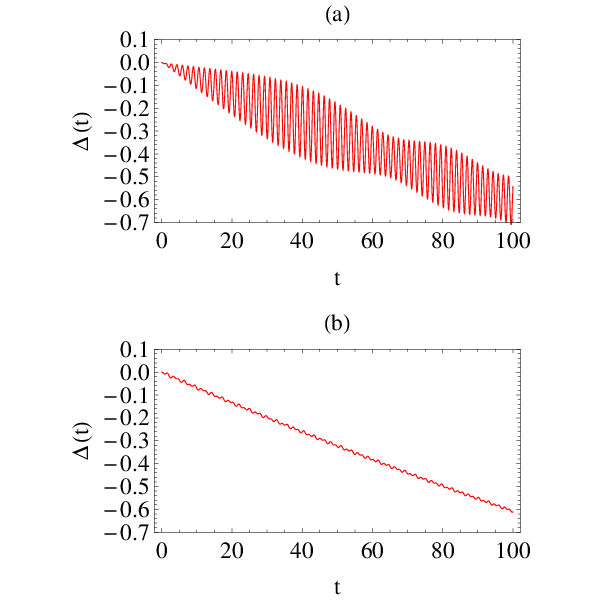
Before ending this section we should note once again the differences between the two times: the Mino-type time parameter and the normal time parameter . With respect to both the oscillations and the oscillations are periodic with frequency and respectively. The corresponding oscillations with respect to -time are not in general periodic. The fundamental frequencies are in this case and . The two types of frequencies are not equal, but the ratio between them is the same, that is
| (113) |
since the ’s frequencies (with respect to ) are simply the components used in the construction of the fundamental frequencies (c.f. Eqs. (169, 170, 174) in Appendix E).
7 Conclusion - Discussion
In this article we have studied thoroughly a Newtonian gravitational field that shares a lot of similarities with the relativistic gravitational field of a Kerr black hole. The fundamental property of both problems that makes them look similar is the fact that both are integrable and separable problems, characterized by three constants of motion, the physical meaning of which is completely analogous in the two cases. These three integrals of motion are the energy, the -component of the angular momentum, and the Carter constant, a quantity that is quadratic with respect to momenta which could be viewed as a continuous transformation of the square of the total angular momentum of the corresponding spherically symmetric fields (monopole Newtonian and Schwarzschild) when the extra parameter is introduced so as to destroy the spherical symmetry while retaining the integrability in the two problems. It is quite intriguing that this parameter has a completely different origin in these two problems: while it represents the spin parameter in Kerr case, it is simply a length in the Euler problem, that defines an imaginary distance between the two half masses governing the axi-symmetric gravitational field. Of course the different physical frame assumed when one studies each problem (the relativistic frame in the former one and the Newtonian in the latter one) introduces restrictions in considering the two problems as completely analogous. For example the horizons in Kerr are absolutely absent in the Euler problem since they are of completely relativistic origin. Also the consideration of space-time as a dynamic entity in the Kerr field leads to the dragging of frames, which has no analogue in the Newtonian frozen space of the Euler problem.
We have attempted to give a complete list of properties of the two problems that are qualitatively (and sometimes quantitatively) comparable, taking into account their intrinsic differences. In some parts of our comparison we found a way to bridge these differences; the frame-dragging effect has been artificially neutralized, by considering the rotational frequency of a test body with respect to a ZAMO observer as a physical tool to construct equivalent prograde and retrograde orbits in Kerr, so that the physical characteristics of each such pair could be compared, on equal footing, with the omni-directional orbits in the Euler potential. With respect to other fundamental differences, like the existence of horizons in Kerr, we have avoided to approach such regions by considering only orbits that are bound in a fixed region of the gravitational field in both problems without reaching either the plunging region of the Kerr field, or the interior allowed region of the Euler field. Schematically, we have named the orbits that either move exclusively in the interior region or in a region that has been produced by a merge of the two regions of the Euler field, “plunging” or “effectively plunging”, as well).
The similarities between the two problems are summarized in the following list: (i) The separability of the two problems leads to two potentials and that describe the orbital dynamics. Both share a lot of common properties: ’s have exactly the same form in both problems, while ’s are described by 4th order polynomials in which the physical constants of motion are introduced in similar but not exactly equal manner (part of the difference is due to the frame-dragging dynamic property of space-time itself which is incorporated in Kerr’s potential). (ii) Due to separability, the wave properties in both fields have analogous characteristics, especially the scalar case. (iii) The multipolar structure of the Euler field is exactly that of Euler, if the current-moments of Kerr are neglected. This makes the two problems behave exactly like each other at least at large distances. (iv) The bound orbits are precessing orbits that move in and out radially. (v) There is an ISCO for both problems. This is of great astrophysical interest since one could describe disks of matter with a finite internal radius. (vi) Although the case of the Euler problem is the monopole gravitational field leading to simple closed elliptical orbits, whatever the initial conditions are, the Eulerian problem has an ISCO and bound orbits that are not closed in the strong field region, which is also true in the Schwarzschild case. (vi) The bound orbits are characterized by a set of three fundamental frequencies in both problems. The expressions for the frequencies could be written in similar forms, in terms of elliptical integrals, for both problems. Especially in the strong field regime analogous characteristics arise. Thus in a specific region of orbital characteristics, both problems have pairs of distinct orbits with the same set of fundamental frequencies.
A simple first exploitation of this unique analogy between the two problems is to consider the Boyer-Lindquist coordinates that are usually used to describe the Kerr metric not as the analogous of spherical coordinates (used in the Schwarzschild case) but rather as some kind of oblate spheroidal coordinates that are suitably adjusted by the spin parameter of the Kerr black hole, which is directly related with the quadrupole moment of the black hole itself. This different view-point elucidates the difference in radial proper distance across the equator and across the axis of symmetry of the Kerr metric.
Also, taking into account all the above similarities, one could use the Newtonian problem as a simple mechanical model to discuss and clarify some subtle issues regarding the dynamics of orbits in a Kerr black-hole field. In this article we have reexamined the old argument according to which the “circular” orbits evolve into circular orbits in Kerr, under the action of a self-force arising from the radiation reaction of EMRIs. The evolution of a “spherical” (as we call it here) orbit in the Euler problem under a generic dissipative self-force has been investigated. We have analyzed the dynamic evolution of radial oscillations under the influence of such an external force and ended up into a simple harmonic oscillator toy-model with a drifting and oscillating frequency driven by a force that is partly linear with respect to time and partly oscillating. Both oscillating parts in this mechanical model have the frequency of , that is twice the frequency and higher even harmonics. According to our toy-model the radial oscillations will grow, mainly due to simple resonance when the resonance condition (with integer) is met. As explained in Section 6 the parametric resonance (corresponding to ), although in principle capable to increase exponentially the eccentricity of the orbit, it is quite sensitive to the resonance condition; consequently it is rather difficult to arise when all frequencies are drifting. On the other hand the simple resonance condition (which is met when ) will make the eccentricity grow linearly with time or it will cause a beating effect when the resonance condition is turned on and off due to frequency drift. This analysis could be used to analyze and explain the adiabatic evolution of a spherical orbit either in Kerr or in Euler under any type of perturbative dissipative external force. While in Kerr the fundamental resonance condition has not been found to hold for any kind of spherical orbits, this is not true for the Euler problem. The small quantitative differences between the two problems render the Euler problem suitable to test our model. Having the analytical tools to seek an orbit in the frequency parameter space with suitable frequencies in resonance, it was quite easy to find such an orbit with initially. Then we numerically evolved it under a small external (non-gravitational) dissipative force of very simple form. We actually confirmed that our mathematical model captures the exact qualitative behavior of the orbital eccentricity.
We believe that the analogy presented in this paper could be further used to study the adiabatic passage of an orbit around a black hole through a resonance due to gravitational radiation. The Euler analogue is a perfect tool, we believe, to thoroughly study such a delicate issue that might have implications in the corresponding signal either in the Kerr case (an exact integrable system), or that of a modified slightly non-integrable system (e.g. a perturbed Kerr black hole) by employing, accordingly, a suitable Newtonian analogue of a modified Euler gravitating system that is constructed to be slightly non-integrable. We plan to address these issues in a following paper.
Acknowledgements
TA would like to thank a lot of people with whom he had long discussions, during the past years, about this problem. Katerina Chatziioannou, and later George Pappas were the first persons who performed the first computations regarding some of the similarities relating the orbital characteristics in Euler and in Kerr. Also Charalampos Markakis who shared with us his ideas with respect to generalizations of the notion of Carter constant. Later Kostas Glampedakis collaborated with TA to investigate the similarities at the level of wave properties. Technical advice from Maarten van de Meent’s who has acquired a deep intuition on Kerr’s resonances was of great help as well. We offer our thanks also to Georgios Lukes-Gerakopoulos for sharing his insightful ideas regarding chaotic behavior of orbits in non-integrable systems with us. AE would like to thank the research funding program I.K.Y. (MIS-5003404) for its support, which was of great importance for the completion of this research project.
Appendix A Oblate Spheroidal coordinates
The Lagrangian in oblate spheroidal coordinates is:
| (114) | |||||
where ( is the radial oblate spheroidal coordinate). An overdot denotes differentiation with respect to time coordinate .
From Euler-Lagrange equations, we derive the equations of motion:
| (115) | |||||
| (116) | |||||
| (117) |
We used the above equations for integrating numerically the orbits and not Eqs. (34)-(36). When the latter ones where used in a numerical integration scheme, Eqs. (34)-(36) accumulate error at the turning points due to the square roots. Moreover the signs of the and velocities have to be changed every time the orbit passes through a turning point.
The oblate spheroidal unit vectors are [29]:
where are the Cartesian unit vectors. Finally the position vector is:
| (118) |
while the velocity vector expressed in terms of oblate spheroidal coordinates is:
| (119) |
Appendix B Parameterization of orbits
The potentials of Eq. (37) and of Eq. (38), that govern the bound motion, could be rewritten as:
| (120) |
| (121) |
Note the here is the initial Eulerian energy before, its substitution by the corresponding relativistic analogue. The radial potential has either four real roots with order or two real roots with order and two complex conjugate roots . The roots of longitudinal potential are which satisfy the inequalities and . Normal bound orbits have and . We have excluded from our study bound orbits with (considering them plunging orbits), while does not correspond to any physical value.
At numerical calculation we have used the orbital parameters as a useful parametrization of bound orbits. Where is the eccentricity, is the semi-latus rectum and is the lowest polar angle along the orbit. The turning points of a normal bound orbit become:
| (122) |
The rest of the roots of the potentials (120) and (121) can be computed from the form of the polynomials and the corresponding constants of motion . Analyzing (120) and equating to (37) we obtain the following equations:
which end up to the following expressions:
| (123) |
where
| (124) |
and
| (125) |
Also, equating (38) and (121) we find:
which gives:
| (126) |
Next we need to express the constants of motion , showing up in the expressions above, in terms of the orbital parameters . For the Kerr space-time, similar expressions have been given by Schmidt in Appendix B of [25]. We use the condition of turning points () at to express as a function of :
| (127) |
and rewrite the radial potential as:
| (128) |
where the functions:
Furthermore we impose at and . (For circular orbits with we should solve simultaneously the equations and at .) The energy and angular momentum are then given by:
| (129) | ||||
| (130) |
where we the determinants are defined as:
| (131) | |||||
| (132) | |||||
| (133) |
In the above expressions for the determinants the subscripts 1, 2 have the following meaning:
- i.
for eccentric orbits ():
(134) (135) - ii.
for circular orbits ( and ):
(136) (137)
In total, starting from the three orbital parameters : (a) we construct the determinants , using Eqs. (131-133), (b) from them we compute the constants of motion and through Eqs. (129, 130, 127), and (c) we finally obtain the four radial roots of (from Eq. (123)) and the second root, , of (from Eq. (126)).
Appendix C Separatrix
The separatrix describes all orbits that are essentially circular although their eccentricity is not necessarily zero. It is defined as the set of orbits with . Due to this double root the orbit spends infinite time to approach this root, therefore it evolves into an eternally circular orbit.
In this Appendix we parametrize these orbits by two parameters (the eccentricity) and . From these two parameters we will show that one could construct the rest orbital parameters , as well as the constants of motion . We will show also that the new parameter is intimately related to the inclination of the orbit. Thus for the orbit is equatorial (), while for we get the maximally inclined orbit ().
Let’s start from the radial potential (37):
| (138) |
which is a polynomial of degree four:
| (139) |
where the roots are given in Appendix B. The motion of a particle is restricted between (Section 3.2). On separatrix, . The smallest root , always lies within the interval thus , where . Equating the coefficients of the polynomials (138), and (139) and introducing the above parametrization for we derive the following set of equations:
| (140) | ||||
| (141) | ||||
| (142) | ||||
| (143) |
Solving this system of equations we can express the constants of motion and the semi-latus rectrum as functions with respect to the eccentricity and the parameter only:
| (144) |
| (145) |
| (146) |
| (147) |
The is the lower root of the quadratic equation . That is:
| (148) |
where . Replacing (144)-(147) in (148), we obtain:
| (149) |
For a fixed eccentricity , is a monotonically increasing function of . It takes its greatest value at , while for , it is (equatorial orbits), as mentioned earlier. This parameter is not very practical for bound orbits in Kerr, though, since the maximally inclined orbits in Kerr do not correspond to .
Appendix D Fundamental Frequencies
In this Appendix we give analytic expressions that one could use to calculate the fundamental frequencies of normal bound orbits in the Euler field. We will exploit the action-angle variables formalism [10]. We denote the constants of motion as: . The canonical momenta are: , and , with the potentials given in Eqs. (37) and (38). The definition of the action variables, of Eq. (67), give:
| (150) | ||||
| (151) | ||||
| (152) |
In order to derive the corresponding frequencies
we should first express the Hamiltonian with respect to the action variables , which can’t be done analytically. The integrals (150)-(152) of action variables, cannot be explicitly inverted. However, we can calculate the frequencies from the inverse derivatives , combined with the chain rule. The non trivial partial derivatives are:
| (153) | ||||
| (154) | ||||
| (155) | ||||
| (156) | ||||
| (157) | ||||
| (158) |
with , and being the 1st, 2nd and 3rd complete elliptic integrals that are given in Eqs. (77, 78, 79), while the quantities , and are the radial integrals:
| (159) | ||||
| (160) | ||||
| (161) |
Finally the two extra quantities shown above are defined as and . Now we can inverse the derivatives (153)-(158), using the chain rule
| (162) |
By setting we obtain the system of equations:
which solved with respect to provides us with the desired frequencies:
| (163) | ||||
| (164) | ||||
| (165) |
Although the denominators of the integrals (159, 161) vanish when the orbit passes through a turning point, Mathematica is capable to campute the above frequencies. We should note that the above expressions for the fundamental frequencies are identical to those for Kerr orbits (c.f. [25]), except of the actual form of and the form of the integral .
Appendix E Alternative analytical expressions for the frequencies
We should emphasize the fact that the expressions for the fundamental frequencies derived in Appendix D, directly from the formalism of action-angle variables turn into indefinite expressions when (separatrix). Then one needs to resort in approximating analytical expressions for this region, which is quite challenging especially for generic orbits. Another major problem is that the and oscillations are not periodic in coordinate time , since the corresponding equations (c.f. Eqs. (34, 35)) are coupled through the quantity . Following [30], in order to decouple the radial and polar motion, we introduce a new time variable,
| (166) |
by analogy with the Mino time, which is widely used in the study of geodesic orbits in Kerr. Then the corresponding variables become strictly periodic with respect to . It is preferable to derive new analytical expressions for the frequencies exploiting the elliptic integrals and the new time variable (166) as Fujita and Hikida did for Kerr.
The geodesic equations in the new time variable become:
| (167) |
where the new functions that are introduced above are:
| (168) |
The frequency of the -motion and -motion, with respect to , will be denoted and , respectively. Similarly, one can define the azimuthal -frequency and the frequency of the coordinate time with respect to . Following the procedure of [30], we derive all frequencies for the Euler problem.
The radial (37) and polar (121) potentials are polynomials of order four for both Euler and Kerr, so and of Euler are exactly the same with that of Kerr, when written in terms of the roots of the corresponding polynomial. We will write the final expressions and not reproduce all the calculations here (the various new quantities introduced here will be analytically presented at the end). The process is exactly the same with that for the Kerr field:
| (169) | |||
| (170) |
while the and for Kerr are defined by Eqs. (7), (8) of [30]. When they are translated into the Euler case they yield the following form:
| (171) | ||||
| (172) |
where:
and denotes the average over . could be recast in the following form
| (173) |
and using the expressions and integrals from Appendix A of [30], we obtain the following expressions for the rest frequencies:
| (174) |
| (175) |
The various quantities that appear on the formulae for the frequencies above are defined as:
| (176) | |||||
| (177) | |||||
| (178) | |||||
| (179) | |||||
| (180) | |||||
| (181) |
while he expressions and are the complete elliptic integrals of first, second and third kind respectively (note that [30] has different conventions for the elliptic integrals than the ones used in this article).
The fundamental frequancies in coordinate time are finally given by:
| (182) | ||||
On the plots of the text all fundamental frequencies of the Euler problem were calculated based on the analytical expressions (182). These formulae are precise and easy to calculate by means of Mathematica even for the region close to separatrix that is when .
Especially at the separatrix the expressions for the frequencies are greatly simplified since the ratios between some elliptic integrals vanish, that is,
| (183) |
and
| (184) |
The final expressions for the frequencies at the separatrix are still given by Eqs. (182), but now the various components ’s and are much simpler:
| (185) | ||||
References
- [1] L. Euler, Nov. Comm. Acad. Imp. Petropolitanae, 10, pp. 207–-242, 11, pp. 152–-184; Mémoires de l’Acad. de Berlin, 11, 228–-249. 1760.
- [2] E.T. Whittaker, A Treatise on the Analytical Dynamics of Particles and Rigid Bodies (4th Edition), Cambridge Univ. Press, 1989.
- [3] R. P. Kerr, Phys. Rev. Lett. , 237 (1963).
- [4] B. Carter, Phys. Rev. Lett. , 331 (1971).
- [5] S. Chandrasekhar, The Mathematical Theory of Black Holes, Oxford Univ. Press, 1983.
- [6] B.P. Abbott et al. (LIGO Scientific Collaboration and Virgo Collaboration), Phys. Rev. Lett. , 061102 (2016), arXiv:gr-qc/1602.03837.
- [7] E. Poisson, A. Pound and I. Vega, Living Rev. Relativity , 7 (2011), arXiv:gr-qc/1102.0529.
- [8] B. Carter, Commun. Math. Phys. , 280 (1968).
- [9] K. Rosquist, T. Bylund and L. Samuelsson, Int. Journal.of Mod. Phys. D , 429 (2009).
- [10] V. I. Arnold, Mathematical Methods of Classical Mechanics (2nd Edition), Springer, New York, 1989.
- [11] C. M. Will, Phys. Rev. Lett. , 061101, (2009).
- [12] D. Kennefick and A. Ori, Phys. Rev. D , 4319 (1996), arXiv:gr-qc/9512018.
- [13] G. Lukes-Gerakopoulos, T. A. Apostolatos and G. Contopoulos, Phys. Rev. D , 124005 (2010), arXivgr-qc/1003.3120.
- [14] A. N. Kolmogorov, Dokl. Akad. Nauk SSSR 98, 527(1954); V. I. Arnold, Russ. Math. Surv. 18, 13 (1963); J. Moser, Nachr. Akad. Wiss. Göttingen Math.-Phys. Kl. II 1(1962).
- [15] H. Poincaré, Rend. Circ. Mat. Palermo 33, 375 (1912); G. D. Birkhoff, Trans. Am. Math. Soc. 14, 14 (1913).
- [16] L. D. Landau and E. M. Lifshitz, Mechanics (3rd Edition), Butterworth-Heinemann, Oxford, 1976.
- [17] D. Lynden-Bell, MNRAS , 208 (2003).
- [18] W. Israel, Phys. Rev. D , 641 (1970).
- [19] H. Keres, Soviet Phys. JETP , 504 (1967).
- [20] C. Markakis, MNRAS , 2974-2985 (2014), arXiv:gr-qc/1202.5228.
- [21] K. Glampedakis and T.A. Apostolatos, Classical and Quantum Gravity , 055006 (2013), arXiv:gr-qc/1301.3309.
- [22] J.M. Bardeen, W.H. Press and S.A. Teukolsky, Astrophys. J. , 347 (1972).
- [23] K. S. Thorne, R. H. Price and D. A. MacDonald, Black Holes: the Membrane Paradigm, Yale University Press, 1986.
- [24] M. Abramowitz and I.A. Stegun, Handbook of Mathematical Functions, Dover, New York, 1965.
- [25] W. Schmidt, Classical and Quantum Gravity , 2743 (2002), arXiv:gr-qc/0202090.
- [26] T. Hinderer and É. É. Flanagan, Phys. Rev. D , 064028 (2008), arXiv:gr-qc/0805.3337.
- [27] N. Warburton, L.Barack and N. Sago, Phys. Rev. D , 084012 (2013), arXiv:gr-qc/1301.3918.
- [28] F. D. Ryan, Phys. Rev. D , R3159 (1995), arXiv:gr-qc/9506023.
- [29] S. X. K. Howusu, F. J. N Omaghali and F. F. Musongong, Journal of Applied Sciences Volume 7, Number 1 2004.
- [30] R. Fujita and W. Hikida, Classical and Quantum Gravity , 135002 (2009), arXiv:gr-qc/0906.1420.