A Multi-Feature Diffusion Model: Rumor Blocking in Social Networks
Abstract
Online social networks provide a convenient platform for the spread of rumors, which could lead to serious aftermaths such as economic losses and public panic. The classical rumor blocking problem aims to launch a set of nodes as a positive cascade to compete with misinformation in order to limit the spread of rumors. However, most of the related researches were based on one-dimensional diffusion model. In reality, there are more than one feature associated with an object. The user’s impression on this object is determined not just by one feature but by his/her overall evaluation on all of these features. Thus, the influence spread of this object can be decomposed into the spread of multiple features. Based on that, we propose a Multi-Feature diffusion model (MF-model) in this paper, and a novel problem, Multi-Feature Rumor Blocking (MFRB), is formulated on a multi-layer network structure according to this model. To solve MFRB, we design a creative sampling method, called Multi-Sampling, which can be applied to a multi-layer network structure. Inspired by martingale analysis, the Revised-IMM algorithm is proposed, and returns a satisfactory approximate solution to MFRB. Finally, we evaluate our proposed algorithm by conducting experiments on real datasets, and show the effectiveness and accuracy of the Revised-IMM algorithm and significantly outperforms other baseline algorithms.
Index Terms:
Multi-Feature Diffusion, Rumor Blocking, Social Networks, Sampling, Approximation Algorithm, MartingaleI Introduction
The online social platform, such as Facebook, Twitter, LinkedIn and WeChat, have been growing rapidly over the last years, and has been a major communication platform. There are more than 1.52 billion users active daily on Facebook and 321 million users active monthly on Twitter. Usually, these social platforms can be represented as online social networks (OSNs), which is a directed graph, including individuals and their relationship. Even that providing users with convenient information exchange, OSNs provide opportunities for rumor, namely false or negative information, to spread as well. It can cause something bad happening and even panic. For example, in 2013, the fake news ”President Obama is attacked” spread in Twitter caused the US stock falling wildly. Then, in 2016, the rumor made by competitors that ”Hillary Clinton dumped weapons to ISIS” spread in Facebook damaged her reputation in presidential election [1]. In 2018, a video spread in Weibo that a bus fell down into river from a bridge because of a car, leading to there are 15 people losing their lives. In Weibo, All the comments were unanimously pointed to that this tragic tragedy was caused by the driving driving mistakes of the car driver. However, after investigation by the police, the disaster was brought by a dispute between the bus driver and an unreasonable passenger. Thus, the car driver was acquitted immediately.
The influence in social networks is diffused from user to user, which can be initiated by a set of seed (initial) users. The notable study of influence diffusion is traced back to Kempe et al. [2] where influence maximization (IM) problem was formulated as a combinatorial optimization problem: find a subset of users as the seed set that makes the follow-up adoptions maximized by spreading the influence. They proposed two information diffusion models that are accepted by most researchers in subsequent researches: Independent Cascade model (IC-model) and Linear Threshold model (LT-model), and proved IM is NP-hard and its objective function is monotone submodular under these two models, thus, a good approximation can be obtained by natural greedy algorithm [3]. When opposite points of view, negative and positive information, from different cascades are spread at the same time on the same social network, users are more inclined to accept the information arriving on them first. Therefore, one solution of blocking rumor spread is to launch a positive cascade to compete with misinformation [4] [5]. Since the budget for positive seeds is limited, a classical rumor blocking (RB) problem is formulated, which aims to spread a positive cascade by selecting a positive seed set to prevent the spread of misinformation as much as possible.
The existing researches, regardless the problem about IM or RB, were based on the simple IC-model or LT-model. In other words, a piece of information that propagates through the network has only a boolean state, either good or bad. However, in the real world, the actual information diffusion is much more complicated. Let us look at an example first.
Example 1.
For a computer, the features associated with this computer are price, performance, appearance and brand. Whether a user will purchase this computer is determined by his overall evaluation on these features, for example, price is high or low, performance is good or bad and so on.
Therefore, in this paper, we propose a multi-feature diffusion model (MF-model), which matches to the realistic scenario better. For a user, the quality of a product depends on his/her evaluation on the features associated with this product. Information diffusion is not simple one-dimensional, object by object, but multi-dimensional, feature by feature. Back to the above example, someone want to promote this computer, he does not tell others directly that this computer is very good, but tell others that its price is low, performance is satisfactory and so on. In our MF-model, we assume that each feature can be diffused individually. After the diffusion of each feature terminates, users can determine whether this product is good or bad according to their own evaluation criteria. The importance of each feature is different for different users, which strengthens the generalization of model.
Then, we propose a Multi-Feature Rumor Blocking (MFRB) problem, which selects a positive seed set to compete with rumor cascade under the MF-model. The rumor from competitor is possible to spread wrong information on different features in order to lower down the reputation of the product. For example, somebody says the battery performance of iPhone is not good and its price is too expensive, or some presidential candidate’s private life is extravagant. It is worth noting that although there is some negative news, this does not mean iPhone is not a good product or this presidential candidate is not qualified. The judgement for an object depends on the comprehensive evaluation on all features associated with it. Therefore, our MF-model is suitable to solve such problems. The influence spread in MF-model can be constructed in a multi-layer network structure. We prove the objective function of MFRB problem is monotone non-decreasing and submodular. Unfortunately, computing the exact influence is #P-hard [6], thus the objective function is hard to compute despite Greedy algorithm is simple and effective. To estimate the expected influence, they adopt the Monte-Carlo simulation usually, but the computational cost is not acceptable. In order to improve its efficiency, the randomized algorithms based on reverse influence sampling (RIS) popularized gradually [7] [8] [9]. Inspired by this idea, we propose a novel and effective sampling method, called Multi-Sampling, which can be applied to the multi-layer network structure, and we show that this sampling method is effecitve to solve our MFRB problem. Then, based on Multi-Sampling and martingale analysis, the Revised-IMM (Influence Maximization via Martingales) is formulated, whose performance for MFRB problem is as good as Greedy algorithm but much more efficient than Greedy algorithm. Besides, We can implement Revised-IMM algorithm under the different parameter settings according to your requirements for error and running time. Our contributions in this paper are summarized as follows:
- 1.
This is the first attempt to study multi-feature diffusion problem. By learning some real application scenarios, we propose MF-model to simulate multi-feature diffusion. Then, we show that MF-model can be constructed on a multi-layer network structure.
- 2.
MFRB problem is formulated based on MF-model, and we prove its objective function is monotone non-decreasing and submodular.
- 3.
We design a novel sampling method, Multi-Sampling, which can be applied to multi-layer network structure. Based on Multi-Sampling and martingale analysis, the Revised-IMM is formulated, which returns a -approximate solution of MFRB problem, and runs in expected time.
- 4.
Our proposed algorithms are evaluated on real-world datasets. The results show Revised-IMM is much faster than Greedy algorithm and almost get the same performance for MFRB problem.
Organiztion: In Section II, we survey the related works about RB and its algorithms. We then present MF-model and MFRB problem in Section III, introduce our sampling technique on multi-layer network in Section IV, and design our randomized algorithms in Section V. Finally, we conduct experiments and conclude in Section VI and Section VII.
II Related Works
The RB problem was first proposed by Budak et al. [4]. They presented a multi-campaign IC-model, and showed that RB can be generalized to the submodular maximization problem. Then, they proved that the objective function of RB is submodular and obtained a constant approximation ratio through greedy strategy. He et al. [10] considered the competitive LT-model for RB problem and designed a -approximation algorithm. Fan et al. [11] proposed the least cost RB problem under the opportunistic one-active-one model and obtained a valid theoretical bound. Then, they considered RB problem under the time constraint, constrained by a deadline [12]. In addition to spreading positive cascade, there were two other methods for RB. One was protecting the most influential nodes from influenced by rumor cascade so that the influence of negative information can be reduced [11] [13] [14]. The other was removing some of relationships (edges) that play a central role in networks to limit the spread of misinformation [15] [16] [17]. Other researches about removing nodes or edges to block rumor, please reference [13] [14] [15] [16] [17]. Please read the Srijan’s comprehensive survey [18] if you are interested in more problems about misinformation.
After Kempe’s seminal work [2], a large number of related researches have been done. They try to overcome the high time complexity of Greedy algorithm. It is #P-hard [6] [19] to compute the exact influence of a seed set under the IC-model and LT-model. Monte-Carlo simulation was adopted by many researchers to estimate the expected influence, but the computational cost was unacceptable when applied to large networks. Becasue of the low efficiency of Monte-Carlo simulation, a lot of researchers attempted improve the computational efficiency or overcome the Monte-Carlo simulations [20] [21] [22] [23] [24] [25] [26]. For example, Leskovec et al. proposed an CELF algorithm [20] with a lazy-forward evaluation, which avoids unnecessary computation by estimating the upper bound of influence. CELF++ [21], an improved verson of CELF, reduced its time complexity. The effect was not satisfactory until the emergence of RIS. Reverse influence sampling (RIS) was proposed firstly by Brogs et al. [7], then a series of efficient randomized algorithm arised like TIM/TIM+ [8], IMM [9] and SSA/D-SSA [27]. They were scalable methods with -approximation guarantee for the IM problem. Recently, Li et al. [26] proposed TIPTOP based on RIS, an almost exact solutions for IM in in Billion-Scale Networks, which tried to reduces the number of samples as much as possible. Inspired by them, Tong et al. [5] presented an efficient randomized algorithm for RB problem, whose sampling technique is called Random R-tuple. Besides, in order to improve time performance better, Tong et al. proposed a novel sampling method, hybrid sampling technique [28], which attached high weights to the users who are prone to be affected by rumor instead of sampling the nodes uniformly.
III Problem Formulation
In this section, we introduce the MF-model and formulate the MFRB problem.
III-A Influence Model
A social network can be given by a directed graph where is the set of users, is the set of directed edges which describe the relationship between users. The node set and edge set for graph can be referred as and , respectively. For an edge , is an incoming neighbor of and is an outgoing neighbor of . We use and to denote the set of incoming neighbors and outgoing neighbors of node , respectively. To simulate the diffusion process, there are two classical diffusion models, IC-model and LT-model, proposed by Kempe et al. [2].
Definition 1 (IC-model).
It assumes that when a node is activated in this round, in the next round, which can execute an activation attempt to activate those inactive nodes in its outgoing neighbors with a predefined probability. Each edge is associated with a activation probability and the activation process of different edges or different round is independent. Finally, the diffusion process stops if there is no nodes can be activated in future.
Definition 2 (LT-model).
It assumes that each edge is associated with a weight and each node has a threshold distributed in uniformly. For each node , we require that , and define as the set of active incoming neighbors to node . The node can be activated in this round when satisfying . Finally, the diffusion process stops if there is no nodes can be activated in future.
Next, the monotonicity and submodularity can be defined here. We say that a set function is monotone if for any subsets , . A set function is submodular if for any and , the marginal gain of when added to is less or equal to that when added to . That is, .
III-B Realization
Given a dircted graph , a realization is a subgraph of satisfying that and . Under the IC-model, the diffusion probability of those edges in the realization is equal to . Those edges in are referred as to live edges, otherwise, called blocked edges. Under the IC-model, for each edge , it appears in realization with probability . Let be the probability of realization generated from under the IC-model, we have
| (1) |
Obviously, there are possible realizations in all. The diffusion process in a realization is a deterministic process. Thus, we can think about the propagation process from two different perspectives. Given a seed set , the diffusion process can be considered as a stochastic propagation process on graph , or a deterministic propagation process on a realization generated from .
In classical IM problem, we usually denote by the expected number of active nodes (influence) given a seed set . Under the IC/LT-model, we have
| (2) |
where is the set of all realizations generated from and is the number of nodes for which there is a directed path of live edges from a node in in the realization .
Lemma 1 ([2]).
The objective function is monotone non-decreasing and submodular under the IC/LT-model.
Remark 1.
The function is a general notation to represent influence function, thus, every time we mention it, we need to emphasize which diffusion model it is based on.
III-C Problem Definition
First, let us consider a scenario with composed influence under a single cascade. Considering a product with features and a directed social network , the diffusion process can be regarded as discrete steps:
- 1.
Each node represents a user, and there are two possible states associated with each user, active and inactive. The user is active when he/she is willing to purchase this product. Initially, all users are inactive.
- 2.
Each edge is associated with a -dimensional probability vector , where represents the activation probability of feature . When user is activated, he/she will attempt to motivate his/her inactive outgoing neighbor to accept feature with probability . In this activation attempt, maybe will accept one or many features.
- 3.
If user receives influence from more than one active incoming neighbors simultaneously, will treat their features independently.
- 4.
Each user has a threshold , representing the threshold that will purchase this product, and a weight vector , where represents the weight of feature and . User will be activated if and only if the total weight of accepted features is larger than or equal to .
- 5.
Initially, a seed set, containing initial users, is activated. At each step, every user checks whether the activated condition is satisfied. The process ends if no user becomes newly active at current step.
Observation 1.
According to above composed influence model, the expected influence (active nodes) is not submodular.
Proof.
We take a counterexample to show that. Considering a product associated with five features, a user has five incoming neighbors . For each edge , we define and other for . We assume that user has a threshold and weight on each feature . Obviously, and , contradicting the property of diminishing marginal gain. Thus, is not submodular under the composed influence model. ∎
Are there any techniques improving the composed influence to make the expected influence be submodular? We assume user will be influenced by the features of his/her incoming neighbor only when is activated. This condition can be relaxed. Here, each feature can be spread individually, in other words, can be influenced by the accepted features of , but is inactive. Thus, we can treat this relaxed diffusion model as a multi-dimensional IC-model. That is, each feature diffuses in its own dimension like the diffusion of IC-model and consults with other dimensions only when making decision to purchase the product. In order to simulate the real scene better, the threshold should be distributed in interval uniformly. In this paper, we assume that the weight for feature is equal for different users, . This property is useful to prove the submodularity later. So far, the revised composed influence model, called Multi-Feature Diffusion Model (MF-model), is formulated as follows:

Definition 3 (MF-model).
Given a product with features and a directed social network , there exists an equivalent directed multi-layer graph . For each feature , make a copy of . Here, we define in is the copy of corresponding node in . The new graph . For each edge , the activation probability is equal to defined in composed influence model. For each layer , only feature is spread on it and the diffusion process in this layer is independent to other layers. After all diffusion terminate, we need to determine whether a user is activated. Here, we define if node accepts feature , otherwise . If user satisfies the following condition:
| (3) |
we say this user is activated. Other definition is similar to that in composed influence model.
Remark 2.
The nodes in are called user node, or user; but the nodes in are called feature node, or feature. For example, a user node corresponds to feature node set . A user node can be activated when satisfying Equation (3). To avoid confusion, we say a feature node is accepted when it is activated in its layer.
Then, we take an example, shown as Fig. 1, to demonstrate how MF-model works. The example in Fig. 1 is a realization of multi-layer graph , and corresponds to three features. Initially, user is activated, namely features are accepted. After diffustion stops, for user , feature and are accepted. Assuming , we have , thus, user is activated.
From now, we consider the MF-model as information diffusion model, and there are multiple cascades diffusing on the same social network. A user is -active if he/she is activated by cascade . Initially, all users are -active. Shown as Definition 3, each feature diffuses independently, and then, we are able to determine whether the user is active after all feature diffusions have terminated. Let us consider the following scenario: there are two cascades spreading on network , the positive cascade and the negative (rumor) cascade . Given the rumor seed set , we want to launch a positive cascade to compete against the rumor cascade. Denote by the seed set of positive cascade. The information from and diffuses simultaneously under the MF-model. On the layer , if two opposite cascades activate a node successfully at the same time, rumor cascade has a higher priority. That is, will be -accepted. After all feature diffusions have terminated, we are able to determine whether a user is -active or -active.
Remark 3.
For a user , we define as ’s corresponding feature nodes. Assuming that a seed set is served for cascade , we say is partially -active if there exists some user , only part of feature nodes in accept cascade . For example, only accept cascade . On the contrary, is fully -active if all feature nodes of each user in accept cascade . Then, we denote by , , the set of corresponding feature nodes of in layer that accept cascade . If is partially -active, then . If is fully -active, then .
In the real world, a user can hardly be so stupid that he/she believes the rumor that announces all the features of a product are not good. Thus, we assume that rumor seed set is partially -active, in other words, there exists some user who does not believe all the features of this product are bad when rumor is this product is totally bad. And positive seed set is fully -active. A user is -active if he/she is not -active. For user , we define if node accepts rumor cascade, otherwise . If user satisfies the following condition:
| (4) |
this user is not activated by rumor cascade. If Inequality (4) is satisfied, we say this user is -active. Besides, we denote by the expected number of -active users given a positive seed set . So far, the Multi-Feature Rumor Blocking (MFRB) problem is formulated.
Definition 4 (MFRB).
Given a social network , a positive integer and a partially -active rumor set , MFRB selects an fully -active positive seed set , , from to make the expected number of -active users maximized under the MF-model. We have
| (5) |
Theorem 1.
In MFRB problem, the expected number of -active users is monotone non-decreasing and submodular with respect to .
Proof.
In order to prove this theorem, we need to represent mathmatically, firstly. The under the MF-model can be defined as follows:
| (6) |
where is the number of feature nodes that cannot be reached by rumor cascade from in the realization of graph , and is the set of feature nodes in layer corresponding to users in according to fully active assumption of .
Then, is the average number of feature nodes, which is -accepted in feature . Becuase the threshold is uniformly distributed in and , each -active node contributes to the expectation of -accepted users. In other words, the probability of user terminated as -active increases by , so increases by . In addition, is monotone non-decreasing and submodular, which has been proven by Tong et al. [5]. is a linear combination of , thus, is monotone and submodular with respect to . ∎
IV Sampling Technique
In last section, we have proven that the MFRB problem is monotone non-decreasing and submodular, thus, the simple greedy algorithm can get a -approximation solution [3]. However, the computational cost of greedy algorithm is too high because computing the objective function of MFRB is #P-hard [6]. Therefore, it is not advisable to compute directly, instead of that, we can find an estimator of by some sampling techniques, and then make this estimator maximized. Here, we will get help from Random R-tuple sampling technique, provided by Tong et al. [5], to design our estimator. First, we define the expected -accepted feature nodes in layer as :
| (7) |
For any feature node , we use R-tuple sampling technique [5] on graph given rumor accepted set , here, we call it as R-sampling. Given as a realization of , feature node and rumor accepted set , the R-sampling is shown as Algorithm 1, which is a little different from the original version in [5]. The R-sampling starts from in and determine whether the incoming neighbors of the nodes in can be added to in a breadth-first searching until one of the rumor nodes in is reached or no node can be furthered reached. Then, the random R-sampling in graph can be generated by the following steps:
- 1.
Select a node from uniformly.
- 2.
Generate a realization of .
- 3.
Get an R-sampling returned by Algorithm 1, R-sampling
This process, called Single-Sampling, is shown as Algorithm 2. Intuitively, contains the feature nodes that could prevent in from influenced by rumor set when one of them accepts positive cascade. For any positive seed set , we define:
| (8) |
Remark 4.
For convenience, we can consider positive seed set as and rumor seed set as .
Here, it is easy to know that because when . Under the set , we generate a collection of Single-Sampling given the feature . We define , the fraction of Single-Sampling in covered by , as follows:
| (9) |
Lemma 2 ([5]).
Given and for feature , we have for .
So far, we have obtained an unbiased estimator for , but it cannot be applied to solve our FMRB problem directly because multiple features exist in our problem. We can consider this problem in another way. Given and rumor seed set , , we select a feature node from these nodes randomly. After confirming this feature node we select belongs to feature , we generate a realization of and then get a R-sampling returned by Algorithm 1. We call this process as Multi-Sampling, which is shown as Algorithm 3. Let be a collection of Multi-Samplings, , that contains Multi-Samplings. We define , the weighted average fraction of Multi-Samplings in covered by , as follows:
| (10) |
Theorem 2.
Given and rumor seed set , we have for .
Proof.
In Algorithm 3, we select a node from uniformly, which means that the average number of Multi-Samplings in generated by a node in each feature is the same. We define the number of Multi-Samplings in generated by a node in feature as , thus, for . Therefore, can be expressed as
| (11) |
According to Equation (10) and (11), for , we have the following observation:
From above, we know that is an unbiased estimator to . Then, the theorem is proved. ∎
V The Algorithm
From the last section, over can be used as an unbiased estimator of objective function . Before designing our algorithm, we need to introduce martingale and its relative properties first, defined as follows:
Definition 5 (Martingale [29]).
A martingale is a sequence of random variables , such that and for any .
Consider a collection of Multi-Samplings, . Let , we define as
| (12) |
where . Becasue of the linearity of expectation, , we have and . The value of is independent to the value from to , thus, . Therefore, is a martingale.
Lemma 3 ([29]).
Let be a martingale, such that , for each and . Then for any , we have
| (13) |
| (14) |
Considering the martingale , we can set because and for each . Here, we define the maximum weight over all features as . Obviously, we have because for each Multi-Sampling , which can only be covered by one kind of feature nodes. If , then we have for . Based on the properties of variance and Equation (12), we can set because
| (15) | ||||
where the Inequality (15) holds because of the above analysis. If , then we have for . Thus, , so . Then, we have following two inequality for any according to Equation (13) (14):
| (16) | ||||
| (17) | ||||
Borrowed from the idea of IMM algorithm [9], our solution of MFRB problem can be designed, which consists of two stages as follows:
- 1.
Sampling Multi-Sampling: This stage generates Multi-Sampling iteratively and put them into until satisfying a certain stopping condition.
- 2.
Node selection: This stage adopts greedy algorithm to drive a size-k user set that covers sub-maximum weight of Multi-Samplings in .
V-A Node Selection
Let be a collection of Multi-Samplings and be the weighted average fraction of Multi-Samplings in covered by . The node selection stage is shown in Algorithm 4. Here, we define the optimal solution as and optimal value as . Because is monotone non-decreasing and submodular, which guarantees that returned by Algorithm 4 satisfies .
Lemma 4.
Given rumor seed set , is monotone non-decreasing and submodular with respect to .
Proof.
First, we show is monotone non-decreasing. For any positive seed set and node , we have
| (18) | ||||
It is monotone non-decreasing becuase implies , . Next, we show is submodular. Given any and , it is equivalent to prove according to Equation (18). Here, we need to show that whenever , which implies and . means that and because of . Then, means that , so . Therefore, and is submodular, the Lemma is proved. ∎
Lemma 5.
If the number of Multi-Samplings in of Algorithm 4 satisfies that ,
| (19) |
then, holds with at least probability.
Proof.
See Appendix A. ∎
Lemma 6.
If the number of Multi-Samplings in of Algorithm 4 satisfies that ,
| (20) |
then, holds with at least probability, where .
Proof.
See Appendix B. ∎
Theorem 3.
Given any , and with , if the number of Multi-Samplings in of Algorithm 4 satisfies that , it returns a -approximate solution of MFRB problem with at least probability.
Proof.
By Lemma 4 and Lemma 5, they hold with probability. Then, . The Theorem is proved. ∎
From Theorem 3, we need to compute and ensure contains at least Multi-Samplings. In order to derive such a , which is feasible to find the minimum . Here, we set and such that . We define as
| (21) |
and . We can verify easily. However, it is difficult to compute the value of directly. In the next subsection, we will find a lower bound of optimal value instead of and determine the number of Multi-Samplings in by .
V-B Sampling Multi-Sampling
In last subsection, we have obtained the approximate minimum value of . Inspired by the idea of IMM algorithm [9], we aim to make the difference between LB and OPT as close as possible. The process of Sampling Multi-Sampling stage is shown in Algorithm 5. In iteration , we generate a certain number of Multi-Samplings, put them into and call Algorithm 4, then compare this result with statistical test . When the LB is close to OPT enough, it terminates the for-loop with a high probability. Obviously, the Multi-Samplings generated by Algorithm 5 are not independent, because those Multi-Samplings generated in iteration are determined by whether the size of collection in iteration is large enough to make the estimation accurate. It can be analyzed by use of martingale technique, which is shown as Lemma 7 and Lemma 8. Finally, we generate a new collection of Multi-Samplings, and we will explain why we need to do that later.
Lemma 7.
Consider the iteration in Algorithm 5, if the number of Multi-Samplings in satisfies
| (22) |
If , then holds with at least probability.
Proof.
See Appendix C. ∎
Lemma 8.
Consider the iteration in Algorithm 5, if , then holds with at least probability.
Proof.
See Appendix D. ∎
Theorem 4.
Given , the number of Multi-Samplings returned by Algorithm 5 satisfies with at least probability.
Proof.
In [30], Chen pointed out this theorem cannot be obtained directly by combining Lemma 7 and Lemma 8. The multi-Samplings generated in iteration are biased samples, because of the fact that the algorithm enters the iteration means that the size of collection in iteration cannot satisfy the termination condition. The complete proof is in the appendix of [30]. Based on that, Theorem 4 is established. ∎
V-C Time Complexity
In the rest of this section, we discuss the time complexity of Algorithm 5. We can observe that the computational cost of Algorithm 5 mainly concentrates on the generation of Multi-Sampling. First, we need to analyze the time of generating a Multi-Sampling. At the high level, we use breath-first search from a feature node to visit each of its incoming neighbors until reaching a rumor node. Thus, the expected time needed to generate a Multi-Sampling is , where denotes the number of edges in that are incoming edges to the nodes in .
Lemma 9.
Considering the objective function defined as Equation (7), we have
| (23) |
where is the optimal value of function and is the number of features.
Proof.
We denote by the collection of all possible Multi-Samplings for a feature node . For any Multi-Sampling , we have
The Lemma is proved. ∎
Lemma 10.
Algorithm 4 runs in time.
Proof.
The running time of Algorithm 4 can be derived directly from Eqaution (10). ∎
Shown as above, the total number of Multi-Samplings generated in Algorithm 5 is . We denote by the ending iteration of the for-loop, we have and where . The expected number of Multi-Samplings generated in Algorithm 5 can be expressed as , thus
| (24) |
From above, we can know that the expected time of generating all Multi-Samplings in Algorithm 5 is . Based on Theorem 3 in [9], another property of martingale [31], we have . Thus,
| (25) |
due to the fact that . Besides, because for any . Thus, the total running time is . Then, we have the following theorem:
Theorem 5.
Algorithm 6 can be ganranteed to return a -approximate solution of MFRB problem with at least probability, and runs in expected time.
Proof.
In [30], Chen pointed out a direct combination of Theorem 3 and Theorem 4 is problematic. For Theorem 3, it is correct given a fixed value of , which means that these Multi-Samplings are sampled from the same sample space. Theorem 4 is based on the satisfaction of Theorem 3, and it uses the same base sample from the probability space. In section 2.4 of [30], Chen proved its correctness of that and provided us with two solutions in section 2.5. Here, we choose the first solution for our MFRB problem: regenerating a new collection of Multi-Samplings. In line 18 of Algorithm 5, after determining the size of , we regenerate a new collection of Multi-Samplings with the length of , from line 19 to line 22 of Algorithm 5, and feed it into Algorithm 4 to get the final result. In section 3.1 of [30], Chen proved that it is bounded with at least probability, which answered the question mentioned above why we need to generate a new collection of Multi-Samplings. ∎
VI Experiment
In this section, we will show the effectiveness and efficiency of our proposed algorithms on three real social networks. Our goal is to evaluate Algorithm 5 and Algorithm 6 with some common used baseline algorithms.
VI-A Dataset description and Statistics
Our experiments are relied on the datasets from networkrepository.com [32], an online network repository. There are three datasets used in our experiments: (1) Dataset-1: A co-authorship network, where each edge is a co-authorship among scientists to publish papers in the area of network theory. (2) A Wiki network, which is a who-voteson-whom network collected from Wikipedia. (3) Dataset-3: an Advogato online social network, which is a social community platform. Users can express weighted trust relationships among themselves explicitly. These datasets contain a list of all of the user-to-user links. Basic statistics of these datasets are summarized in Table 1. However, according to the multi-layer structure of MF-model, the number of feature nodes is dfferent from these basic information. Thus, the actual number of nodes and edges is determined by the number of features. we will describe in detail later.

(a) sub-case: two features

(b) sub-case: three features

(c) sub-case: four features

(a) sub-case: two features

(b) sub-case: three features

(c) sub-case: four features
| Dataset | n | m | Type | Average degree |
|---|---|---|---|---|
| dataset-1 | 0.4K | 1.01K | directed | 4 |
| dataset-2 | 1.0K | 3.15K | directed | 6 |
| dataset-3 | 6.5K | 51.3K | directed | 18 |
VI-B Experimental Setup
The experiment is based on MF-model, thus, the probability on the edges is either set as a constant or for each edge , we set . This setting is widely used in prior works [8] [21] [33]. We call these two setting as constant probability model (CP-model) and weighted cascade model (WC-model). Then, we compare our proposed algorithms with some common baseline algorithm, which is shown as follows:
- •
Revised-IMM: This is the algorithm proposed in this paper, unless otherwise specified, we set and by default.
- •
Greedy: At each step, it selects a node such that adding this node to current seed set can obtain the maximum marginal gain. It is implemented by Monte-Carlo simulation. We set the number of simulations to . It is only tested on small networks, dataset-1 and dataset-2, because of its low efficiency.
- •
Proximity: It selects the outgoing neighbors of the nodes in rumor set according to the out-degree of these outgoing neighbors. We select these neighbors with high out-degree in priority.
- •
Random: This is a classical baseline algorithm, where the nodes in positive set are selected randomly.
In our experiment, the users in rumor seed set are the nodes with the highest outgoing degree in original graph and the size . Because the is partially -active, only part of features of those users in are -accepted, thus, we set the probability that the corresponding feature nodes of accept rumor cascade is . The number of users in positive set is from to , and is fully -active, so the corresponding feature nodes of are all -accepted.
Next, we evaluate the performance of Revised-IMM algorithm. It can be divided into three sub-cases: (a) Assuming for each product, there are two features 1 and 2, the corresponding graph has two layers, one is feature 1 and the other is feature 2. For CP-model, the diffusion probability for feature 1 is and feature 2 is . The weight for feature 1 is and feature 2 is . The actual number of nodes and edges will be doubled. (b) Assuming for each product, there are three features 1, 2 and 3, thus, has three layers for each feature. For CP-model, the diffusion probability for feature 1 is , feature 2 is and feature 3 is . The weight for feature 1 is , feature 2 is and feature 3 is . The actual number of nodes and edges will be tripled. (c) Assuming for each product, there are four features 1, 2, 3 and 4, thus, has four layers for each feature. For CP-model, the diffusion probability for feature 1 is , feature 2 is , feature 3 is and feature 4 is . The weight for feature 1 is , feature 2 is , feature 3 is and feature 4 is . The actual number of nodes and edges will be quadrupled.

(a) sub-case: two features

(b) sub-case: three features
| Dataset-1 | ||||
| Revised-IMM | Greedy | Proximity | Random | |
| (a) | 16.67s | 1.67h | 0.74s | 0.89s |
| (b) | 14.02s | 2.78h | 1.80s | 1.91s |
| (c) | 30.42s | 3.77h | 2.06s | 2.33s |
| Dataset-2 | ||||
| (a) | 148.24s | 19.66h | 4.01s | 3.69s |
| (b) | 167.48s | 32.17h | 6.35s | 6.50s |
| (c) | 193.87s | 41.42h | 8.59s | 8.77s |
| Dataset-3 | ||||
| (a) | 14min | n/a | 2min | 1min |
| (b) | 20min | n/a | 2min | 1min |
VI-C Experimental results
Figure 2 and Figure 3 draw the performance comparison achieved by different algorithms with budget 20 under the dataset-1 and dataset-2. Obviously, we can see that Revised-IMM algorithms and Greedy algorithm have the the same performance with respect to objective function . However, to computational cost, Revised-IMM algorithm is much more efficient that Greedy algorithm. The running time in these experiment is shown as Table II. For example, under the CP-model with , we consider dataset-2 with 4 features, Revised-IMM consumes seconds but Greedy takes about hours.
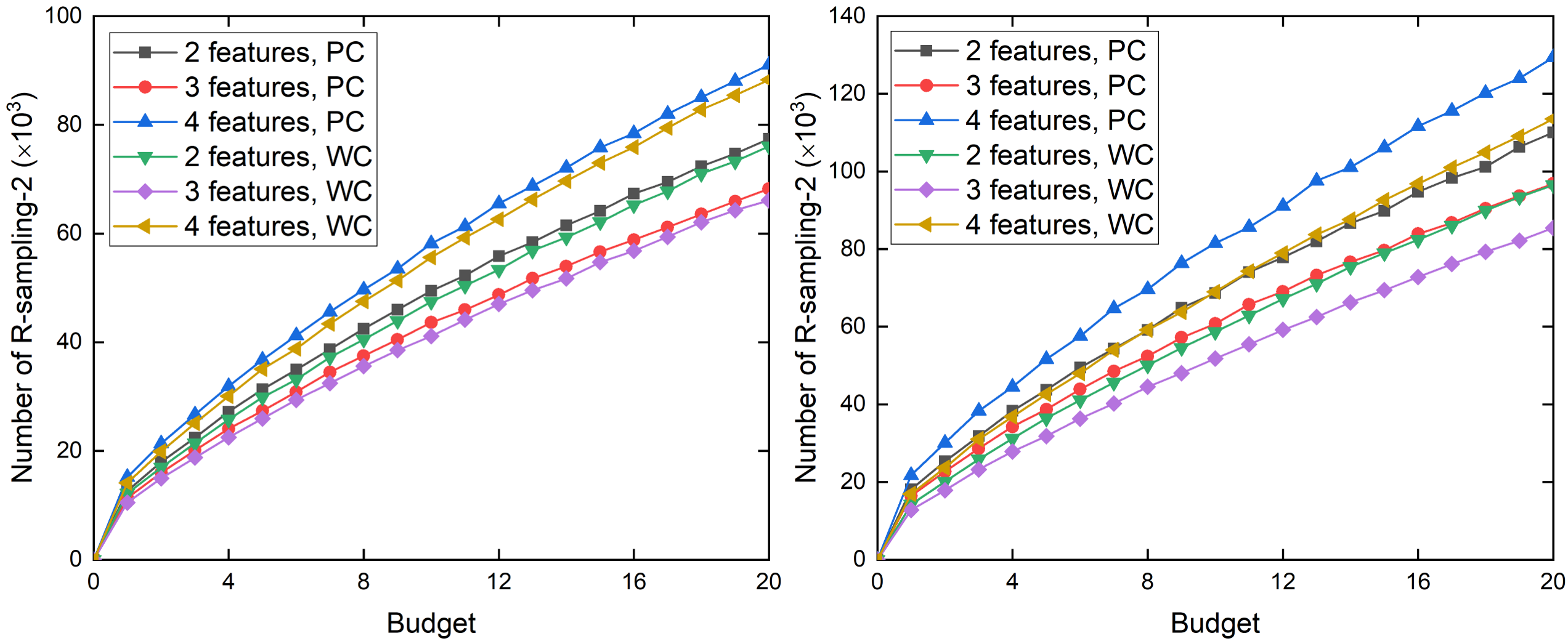
Figure 4 draws the performance comparison achieved by different algorithms with budget 20 under the dataset-3. It verifies the scalability of Revised-IMM algorithm. Figure 5 draws the number of Multi-Samplings generated by Algorithm 5 with different budgets. We can see that this is in line with our expectation, the number of Multi-Samplings increases as the budget increases. Figure 6 draws the average relative error between the estimated value and objective value from budget 1 to 20. Here, given positive seed set and a collection of Multi-Samplings, the estimated value is and objective value is , which is implemented by Monte-Carlo simulation with . Thus, the relative error is . For example, under the setting: dataset-1, , CP-model and 2 features, estimated value is and objective value is , we have relative error is . Therefore, it satisfies what Theorem 2 said, is an unbiased estimator to .

VII Conclusion
In this paper, we propose a novel multi-feature diffusion model, MF-model, to simulate real scenario in which multiple features can be propagated independently in social networks. Based on MF-model, MFRB problem is formulated as a monotone non-decreasing submodular maximization problem. Then, we design a novel sampling technique, Multi-Sampling, which is an unbiased estimator to objective function of MFRB. Inspired by martingale analysis, the Revised-IMM algorithm is proposed, which returns a -approximation solution and runs in expected time. The experimental result verified the effectiveness and correctness of Revised-IMM algorithm.
However, one of the shortcomings of this paper is that the weight for each feature is equal for different users, which is not entirely realistic. Because for different users, the importance of each feature to them is different. For example, some people care more about price, others value the appearance more. In future work, it is worth studying how to solve this more complicated and more realistic situation, which is not submodular, and even not monotone non-decreasing.
-A Proof of Lemma 4
Proof.
For optimal solution , we have defined , thus, . Then, by Equation (16), we have
Thus, holds with at least probability. By Lemma 3 and greedy properties, . The Lemma is proved. ∎
-B Proof of Lemma 5
Proof.
For any -size seed set , we have defined , thus, . Then, by Equation (17) and , we have
Because there exists at most positive size- seed sets and by union bound, there is at least probability that no such that . The Lemma is proved. ∎
-C Proof of Lemma 6
Proof.
For any -size seed set , we have defined , thus, . Then, by Equation (17) and , we know that , and we have
Because there is at least probability by union bound that no such that . The Lemma is proved. ∎
-D Proof of Lemma 7
Proof.
For any -size seed set , we have defined , thus, . Then, by Equation (17) and , we have
Because there is at least probability by union bound that no such that . The Lemma is proved. ∎
Acknowledgment
This work is partly supported by National Science Foundation under grant 1747818.
References
- [1] H. Allcott and M. Gentzkow, “Social media and fake news in the 2016 election,” Journal of economic perspectives, vol. 31, no. 2, pp. 211–36, 2017.
- [2] D. Kempe, J. Kleinberg, and É. Tardos, “Maximizing the spread of influence through a social network,” in Proceedings of the ninth ACM SIGKDD international conference on Knowledge discovery and data mining. ACM, 2003, pp. 137–146.
- [3] G. L. Nemhauser, L. A. Wolsey, and M. L. Fisher, “An analysis of approximations for maximizing submodular set functions—i,” Mathematical programming, vol. 14, no. 1, pp. 265–294, 1978.
- [4] C. Budak, D. Agrawal, and A. El Abbadi, “Limiting the spread of misinformation in social networks,” in Proceedings of the 20th international conference on World wide web. ACM, 2011, pp. 665–674.
- [5] G. Tong, W. Wu, L. Guo, D. Li, C. Liu, B. Liu, and D.-Z. Du, “An efficient randomized algorithm for rumor blocking in online social networks,” IEEE Transactions on Network Science and Engineering, 2017.
- [6] W. Chen, C. Wang, and Y. Wang, “Scalable influence maximization for prevalent viral marketing in large-scale social networks,” in Proceedings of the 16th ACM SIGKDD international conference on Knowledge discovery and data mining. ACM, 2010, pp. 1029–1038.
- [7] C. Borgs, M. Brautbar, J. Chayes, and B. Lucier, “Maximizing social influence in nearly optimal time,” in Proceedings of the twenty-fifth annual ACM-SIAM symposium on Discrete algorithms. SIAM, 2014, pp. 946–957.
- [8] Y. Tang, X. Xiao, and Y. Shi, “Influence maximization: Near-optimal time complexity meets practical efficiency,” in Proceedings of the 2014 ACM SIGMOD international conference on Management of data. ACM, 2014, pp. 75–86.
- [9] Y. Tang, Y. Shi, and X. Xiao, “Influence maximization in near-linear time: A martingale approach,” in Proceedings of the 2015 ACM SIGMOD International Conference on Management of Data. ACM, 2015, pp. 1539–1554.
- [10] X. He, G. Song, W. Chen, and Q. Jiang, “Influence blocking maximization in social networks under the competitive linear threshold model,” in Proceedings of the 2012 siam international conference on data mining. SIAM, 2012, pp. 463–474.
- [11] L. Fan, Z. Lu, W. Wu, B. Thuraisingham, H. Ma, and Y. Bi, “Least cost rumor blocking in social networks,” in 2013 IEEE 33rd International Conference on Distributed Computing Systems. IEEE, 2013, pp. 540–549.
- [12] L. Fan, W. Wu, X. Zhai, K. Xing, W. Lee, and D.-Z. Du, “Maximizing rumor containment in social networks with constrained time,” Social Network Analysis and Mining, vol. 4, no. 1, p. 214, 2014.
- [13] L.-l. Ma, C. Ma, H.-F. Zhang, and B.-H. Wang, “Identifying influential spreaders in complex networks based on gravity formula,” Physica A: Statistical Mechanics and its Applications, vol. 451, pp. 205–212, 2016.
- [14] S. Wang, X. Zhao, Y. Chen, Z. Li, K. Zhang, and J. Xia, “Negative influence minimizing by blocking nodes in social networks,” in Workshops at the Twenty-Seventh AAAI Conference on Artificial Intelligence, 2013.
- [15] E. B. Khalil, B. Dilkina, and L. Song, “Scalable diffusion-aware optimization of network topology,” in Proceedings of the 20th ACM SIGKDD international conference on Knowledge discovery and data mining. ACM, 2014, pp. 1226–1235.
- [16] M. Kimura, K. Saito, and H. Motoda, “Minimizing the spread of contamination by blocking links in a network.” in AAAI, vol. 8, 2008, pp. 1175–1180.
- [17] H. Tong, B. A. Prakash, T. Eliassi-Rad, M. Faloutsos, and C. Faloutsos, “Gelling, and melting, large graphs by edge manipulation,” in Proceedings of the 21st ACM international conference on Information and knowledge management. ACM, 2012, pp. 245–254.
- [18] S. Kumar and N. Shah, “False information on web and social media: A survey,” arXiv preprint arXiv:1804.08559, 2018.
- [19] W. Chen, Y. Yuan, and L. Zhang, “Scalable influence maximization in social networks under the linear threshold model,” in 2010 IEEE international conference on data mining. IEEE, 2010, pp. 88–97.
- [20] J. Leskovec, A. Krause, C. Guestrin, C. Faloutsos, J. VanBriesen, and N. Glance, “Cost-effective outbreak detection in networks,” in Proceedings of the 13th ACM SIGKDD international conference on Knowledge discovery and data mining. ACM, 2007, pp. 420–429.
- [21] A. Goyal, W. Lu, and L. V. Lakshmanan, “Celf++: optimizing the greedy algorithm for influence maximization in social networks,” in Proceedings of the 20th international conference companion on World wide web. ACM, 2011, pp. 47–48.
- [22] W. Chen, A. Collins, R. Cummings, T. Ke, Z. Liu, D. Rincon, X. Sun, Y. Wang, W. Wei, and Y. Yuan, “Influence maximization in social networks when negative opinions may emerge and propagate,” in Proceedings of the 2011 siam international conference on data mining. SIAM, 2011, pp. 379–390.
- [23] H. Zhang, S. Mishra, M. T. Thai, J. Wu, and Y. Wang, “Recent advances in information diffusion and influence maximization in complex social networks,” Opportunistic Mobile Social Networks, vol. 37, no. 1.1, p. 37, 2014.
- [24] J. Ok, Y. Jin, J. Shin, and Y. Yi, “On maximizing diffusion speed over social networks with strategic users,” IEEE/ACM Transactions on Networking (TON), vol. 24, no. 6, pp. 3798–3811, 2016.
- [25] H. T. Nguyen, M. T. Thai, and T. N. Dinh, “A billion-scale approximation algorithm for maximizing benefit in viral marketing,” IEEE/ACM Transactions on Networking (TON), vol. 25, no. 4, pp. 2419–2429, 2017.
- [26] X. Li, J. D. Smith, T. N. Dinh, and M. T. Thai, “Tiptop: Almost exact solutions for influence maximization in billion-scale networks,” IEEE/ACM Transactions on Networking (TON), vol. 27, no. 2, pp. 649–661, 2019.
- [27] H. T. Nguyen, M. T. Thai, and T. N. Dinh, “Stop-and-stare: Optimal sampling algorithms for viral marketing in billion-scale networks,” in Proceedings of the 2016 International Conference on Management of Data. ACM, 2016, pp. 695–710.
- [28] G. Tong and D. Du, “Beyond uniform reverse sampling: A hybrid sampling technique for misinformation prevention,” CoRR, vol. abs/1901.05149, 2019. [Online]. Available: http://arxiv.org/abs/1901.05149
- [29] F. Chung and L. Lu, “Concentration inequalities and martingale inequalities: a survey,” Internet Mathematics, vol. 3, no. 1, pp. 79–127, 2006.
- [30] W. Chen, “An Issue in the Martingale Analysis of the Influence Maximization Algorithm IMM,” arXiv e-prints, p. arXiv:1808.09363, Aug 2018.
- [31] D. Williams, Probability with martingales. Cambridge university press, 1991.
- [32] R. A. Rossi and N. K. Ahmed, “The network data repository with interactive graph analytics and visualization,” in AAAI, 2015. [Online]. Available: http://networkrepository.com
- [33] K. Jung, W. Chen, and W. Heo, “Irie: A scalable influence maximization algorithm for independent cascade model and its extensions,” Tech. Rep., 2011.