Simultaneous multiple-user quantum communication across a spin-chain channel
Abstract
The time evolution of spin chains has been extensively studied for transferring quantum states between different registers of a quantum computer. Nonetheless, in most of these protocols only one sender-receiver pair can share the channel at each time. This significantly limits the rate of communication in a network of many users because they can only communicate through their common data-bus sequentially and not all at the same time. Here, we propose a protocol in which multiple users can share a spin chain channel simultaneously without having crosstalk between different parties. This is achieved by properly tuning the local parameters of the Hamiltonian to mediate an effective interaction between each pair of users via a distinct set of energy eigenstates of the system. We introduce three strategies with different levels of Hamiltonian tuning; each might be suitable for a different physical platform. All the three strategies provide very high transmission fidelities with vanishingly small crosstalk. The protocol is robust against various imperfections and we specifically show that our protocol can be experimentally realized on currently available superconducting quantum simulators.
I Introduction
Spin chains have been proposed Bose 2003 and extensively studied Bose 2007; Nikolopoulos et al. 2014 as data-bus for transferring quantum information between different registers through their natural time evolution. The main advantage of these protocols is their minimal demand for dynamical control and their resilience against disorder and imperfections Petrosyan et al. 2010; Yang et al. 2010. The drawback, however, is the dispersive nature of their dynamics which scrambles the information among various degrees of freedom Eisert et al. 2015; Lewis-Swan et al. 2019. Many proposals have been put forward to fix this issue. By engineering the couplings Christandl et al. 2004; Christandl et al. 2005; Di Franco et al. 2008 or tuning long range exchange interactions Kay 2006 one can achieve a linear dispersion relation and thus fulfill perfect state transfer. Simpler designs excite the system only in the linear zone of its dispersion relation and achieve pretty good transfer fidelities Apollaro et al. 2012; Banchi et al. 2011; Yao et al. 2011. Dual rail systems Burgarth and Bose 2005a; Burgarth and Bose 2005b and -level spin chains Bayat 2014; Qin et al. 2013 can asymptotically reach perfect state transfer. Adiabatic attachment and detachment of qubits Chancellor and Haas 2012; Farooq et al. 2015; Mohiyaddin et al. 2016 and their faster versions through a short cut to adiabaticity Huang et al. 2018; Baksic et al. 2016, optimal control Caneva et al. 2009 and machine learning assisted transfer Porotti et al. 2019 have also been suggested. Routing information between different nodes of a graph can be achieved by a combination of ferro and anti-ferromagnetic couplings Pemberton-Ross and Kay 2011; Karimipour et al. 2012 and encoding the information in a decoherence free subspace protects it against noise Qin et al. 2015. Exploiting projective measurements for encoding Pouyandeh et al. 2014 and countering dephasing Bayat and Omar 2015 can enhance quality of transfer and local rotations Burgarth et al. 2007; Yang et al. 2011 may yield an enhanced communication rate. In addition, an important class of protocols relies on inducing an effective end-to-end interaction between the sender-receiver sites through either weak boundary couplings Wójcik et al. 2005; Venuti et al. 2006; Venuti et al. 2007; Paganelli et al. 2013; Lemonde et al. 2019; Lemonde et al. 2018; Chetcuti et al. or large magnetic fields near the ends Lorenzo et al. 2013; Apollaro et al. 2015. Some of the proposals have been experimentally implemented in coupled optical fibers Bellec et al. 2012; Perez-Leija et al. 2013, nuclear magnetic resonance devices Rao et al. 2014, optical lattices Fukuhara et al. 2013 and superconducting quantum simulators Li et al. 2018.
In almost all the existing state-transfer protocols only one sender-receiver pair can use the spin-chain channel at each time. This significantly reduces the communication rate, a bottleneck that may ultimately limit the speed of big quantum computers. Although multiple qubit communication Apollaro et al. 2015; Chetcuti et al. have been proposed they have no freedom to adjust the choice of the sender and receiver qubits which are predetermined by the symmetry of the system and thus still work as a single sender-receiver protocol with multiple qubits. Alternatively, to increase the rate, bi-directional protocols have been proposed but they have poor fidelities Wang et al. 2011. In classical communication networks (e.g. telecommunication systems), however, the frequency bandwidth of the channel is divided between multiple users who can use the channel simultaneously. This can be achieved by modulating the signal of each pair of sender-receivers with a different carrier signal, each with a distinct frequency, and send it through a common channel. Since each sender’s data lies in a different frequency bandwidth, the corresponding receiver can access the relevant information by using a proper frequency filter. Consequently, crosstalks are prevented and the communication rate is significantly enhanced. A key open question is whether one can develop a quantum counterpart of classical communication systems and allow multiple users simultaneously communicating through a common channel.
In this paper, we address this critical problem by proposing a communication scheme which is based on tuning the local parameters at the sender and receiver sites. These local tunings, proposed in three different strategies, excite different sets of energy eigenstates for communication of each pair of users and thus result in high transmission fidelities and negligible crosstalk. We have also shown that our protocol is stable against various sources of imperfections and propose to implement it on superconducting quantum simulators.
II The Model
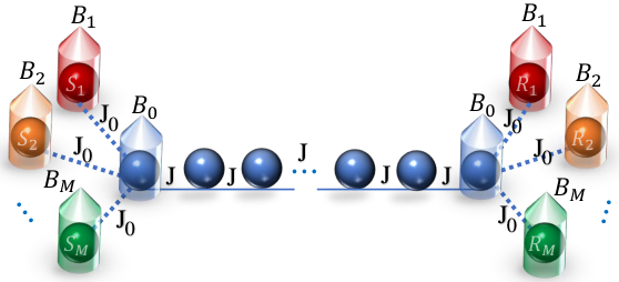
We consider sender-receiver pairs in a way that pair () communicate between the qubits (sender) and (receiver). All pairs share a common spin chain data-bus between their sender and receiver sites. A schematic of the system is given in Fig. 1. The goal is to establish simultaneous high-fidelity communication between any pair of while suppressing the crosstalk between with . The spin chain channel consists of spin- particles which interact via Hamiltonian
| (1) |
where are the Pauli operators acting on site , is the spin exchange coupling and is the magnetic field in the direction acting only on sites and . All senders (receivers) are coupled to the first (last) site of the channel. The interaction between the users’ qubits and the channel is given by
| (2) | |||||
| (4) |
where is the coupling between the users and the channel and is the magnetic field acting on the pair user (see Fig. 1). Without loss of generality, we assume that the sender initially sets its qubit in an arbitrary, possibly unknown, state
| (5) |
where and are the angles determining the quantum state on the surface of the Bloch sphere. The rest of the spins, including all receivers and the channel, are initialized in . Therefore, the state of the whole system becomes
| (6) |
where shows the state of the channel. Since this quantum state is not an eigenstate of the total Hamiltonian , it evolves as . At any time the state of the receiver sites are given by , where means tracing over all sites except .
To quantify the quality of transfer between the sender and receiver we define a fidelity matrix as (), where accounts for the input parameters of the senders. To get an input-independent quantity one can take the average of these fidelities over all possible initial states on the surface of the Bloch spheres for all users
| (7) |
where is the normalized Haar measure. For our Hamiltonian that conserves the total number of excitations, we provide a general form of in Appendix A. The diagonal term quantifies the average fidelity of the transmission between the sender-receiver and the off diagonal term with accounts for the crosstalk between the users and . Our goal is to maximize the transmission fidelities simultaneously and meanwhile keeping the crosstalk fidelities around (i.e. no crosstalk), through controlling the Hamiltonian parameters , and ’s. This goal can be pursue by maximizing the average of the transmission fidelities in time and, consequently, keeping the average of the crosstalks around 0.5. Our protocol can be understood in two steps. The first step is to induce an effective end-to-end transmission between the senders and the receivers, namely confining the excitations to the subspace and leaving the channel close to at all times, by either decreasing Wójcik et al. 2005; Venuti et al. 2006; Venuti et al. 2007; Paganelli et al. 2013; Bayat and Omar 2015 or increasing Lorenzo et al. 2013; Apollaro et al. 2015. The second step is to separate the communication between each of the pairs, by tuning ’s individually. In the following we, first, restrict ourselves to the case of two pairs, i.e. , and consider three different strategies to maximize with minimum crosstalk. Then, we extend the results to larger .
II.1 Strategy 1 ()
In the first scenario, inspired by Ref. Wójcik et al. 2005; Venuti et al. 2006; Venuti et al. 2007; Paganelli et al. 2013; Bayat and Omar 2015 for single user end-to-end communication, we put and consider . This choice of parameters creates an effective direct interaction between the sender subspace and the receiver ones . To suppress the crosstalk and block the flow of information between the two subspaces of and we apply external fields and to make them energetically off-resonant from each other. By sitting at the site one can see the information arrives from both senders. In Fig. 2(a) we plot the average transmission fidelity as function of time in a chain of when the parameters are tuned to , and . As the figure shows, the average transmission fidelity evolves and at a certain time , it peaks to a very high value. In practice, at the receivers need to decouple their qubits from the data-bus or equivalently swap the quantum state from the receiver site to their registers. However, if this decoupling procedure or performing the swap operator happens at a slightly different time then the fidelity may not be at its maximum. However, this error can largely be corrected. The fast oscillations in the average transmission fidelity are due to local magnetic field ’s and the slow dynamics following the envelope of the curve is due to the main Hamiltonian. If the decoupling procedure has a small time delay of then the error is mainly due to fast oscillation and a local rotation of the form on site largely compensates this time delay as it cancels the effect of local rotation by . Interestingly, as Fig. 2(a) shows, the crosstalks remain low and oscillate around resulting in negligible crosstalk between the two communicating parties. Apart from the average fidelity one may also consider the best/worst cases among all possible states which is discussed in details in Appendix B. In order to optimize the parameters, one can fix a time window, e.g. we choose , for the dynamics of the system and then find optimal values for all the Hamiltonian parameters (namely , and ) as well as the time at which all receivers should take their quantum states simultaneously. The corresponding transmission fidelities, for optimal parameters, are . In Fig. 2(b) we plot as well as as functions of . Remarkably, for all channels of length the fidelity remains above , while remains around showing negligible crosstalks. At the chosen time window, the optimal coupling is obtained as for all values of and its weakly depending on the length is consistent with the results of Ref. Bayat and Omar 2015. For the sake of completeness, the optimal time and the optimal local fields , for any given system size are reported in Figs. 2(c) and (d), respectively. The local magnetic fields are chosen from intervals with opposite signs to maximize their difference while keeping their amplitude small. The optimal values for the local fields are not monotonic for different system sizes making the behavior of slightly irregular too.
II.2 Strategy 2 ()
Our second strategy is adopted from Lorenzo et al. 2013; Apollaro et al. 2015 and is accomplished by applying a strong field on the ending sites of the channel and instead keep the couplings uniform, i.e. (see Fig. 1). To see the attainable fidelities for this strategy we plot and as functions of time in Fig. 3(a) for a chain of in which , , and . As the figure shows reaches very high values and peaks at . Remarkably, fluctuates around , showing very small crosstalks. Analogous to the previous strategy, one can optimize the time of the evolution as well as the Hamiltonian parameters within a chosen time window, here again . In Fig. 3(b) we report the maximum of the average transmission fidelity and the average crosstalk as functions of . This figure shows that while the transmission fidelities for both parties achieve above the crosstalks between them remain negligible. The optimal time for obtaining such quantities is plotted in Fig. 3(c). The reason that the optimal times oscillate with length is because the chosen time window allows for several peaks and their maximum changes as the length vary. The other optimal parameters such as and as well as , are presented in Figs. 3(d) and (e), respectively. The results show that by tuning one needs weak local magnetic fields ’s for obtaining high fidelity simultaneous transmission.
II.3 Strategy 3
The third scenario is a hybrid of both outlined strategies and the performance of the channel is investigated when both and are optimized. Again we fix the time window to and optimize the time and the parameters , , , and to maximize the average transmission fidelity and keeping the average crosstalk negligible. In TABLE 1 we report the maximum fidelity , the corresponding crosstalk , the optimal time as well as the optimized values of the Hamiltoninan parameters for different values of . Clearly, and are midway between the two previous strategies, namely becomes larger in comparison with the optimal values in strategy and becomes smaller than the case of strategy . A comparison between different strategies shows that, for long chains strategy is superior to the other ones in terms of fidelity, indicating that a hybrid optimization of both and outperforms the optimization of individual parameters.
| N | 5 | 10 | 15 | 20 | 25 | 30 | 35 | 40 |
|---|---|---|---|---|---|---|---|---|
III Multiple users
The proposed protocol with all the three strategies can be generalized to more than two users. No matter how many users we consider, one can always tune the parameters to keep the crosstalks negligible. To confirm this expectation, we study the performance of two strategies and in the case of three users. Our results show that in different spin chains, three users can simultaneously communicate with the average transmission fidelity more than while keeping the average crosstalk around within the time scale of . In TABLE 2 we report and , the optimal time and also corresponding optimal parameters for some system sizes by adopting the first and second strategies. The transmission fidelities remain steadily high and comparable with the case of two users. Interestingly the optimal coupling strength in the first strategy is obtained as for all considered chains which is very close to the case of users.
| N | 5 | 6 | 7 | 8 | 9 | 10 | 20 | |
|---|---|---|---|---|---|---|---|---|
| N | 5 | 6 | 7 | 8 | 9 | 10 | 20 | |
|---|---|---|---|---|---|---|---|---|
| 0.967 | ||||||||
| 450 | 472 | |||||||
IV Bi-localized eigenstates
The main reason behind the achievement of high transmission fidelities and low crosstalk is the emergence of bi-localized eigenstates whose excitations are mainly localized at sender and receiver sites. Since these bi-localized eigenstates are the only ones involving in the dynamics of the system, the channel mostly remains in the state . Consequently, effective end-to-end interaction is generated between the sender and receiver qubits. The emergence of bi-localized qubits is mainly due to the engineering of and and then, to minimize the crosstalk, further localizing the excitations between each pair is achieved by tuning ’s. See Appendix B for details.
V PERFORMANCE UNDER REALISTIC CONDITIONS
In the previous sections we have illustrated that multiple users can accomplish high-fidelity simultaneous communication with negligible crosstalk by tuning Hamiltonian parameters. However, acquiring this result is based on four ideal assumptions, namely: (i) the chain is initially prepared in the state ; (ii) the couplings are adjusted accurately to their specific values; (iii) the local magnetic fields can be tuned perfectly; and (iv) the system is isolated from its environment. In this section, we investigate imperfect scenarios in which these assumptions are relaxed. For the sake of brevity and without loss of generality, we focus on two-user communication considering only our first and second strategies. Since the third strategy is a hybrid of the first two, the impact of the imperfections will approximately be the average of the impacts on the first two strategies.
V.1 Thermal Initial State
In practice, thermal fluctuations may create excitation in the channel. To investigate the effect of finite temperatures, we consider the initial state of the channel to take the form of a thermal ensemble
| (8) |
where is temperature and is the Boltzmann constant. To see the impact of finite temperature , we compute the average fidelity , for which we provide a compact form in Appendix A. Fig. 4 shows the maximum of transmission fidelities in a chain of length for our first two strategies. As the figure shows, by increasing the temperature the fidelity first remains very high, showing a plateau at small temperatures, and then monotonically decreases to eventually reach the classical threshold of for transferring quantum information Bose 2003. The width of the plateau is determined by the energy gap of the finite system and is consistent with previous observations Bayat et al. 2015. Interestingly, Fig. 4 shows that while the strategy gives higher fidelity at low temperatures, in higher temperatures it is the strategy that gives better transmission quality. Therefore, depending on the temperature of the system one strategy may result in a higher fidelity than the other.
V.2 Random Coupling
The second assumption in our protocols is the homogeneity of the Hamiltonian and tunability of . However, the exchange couplings may not be as precise as we expect and random variations are inevitable during fabrication. For investigating the effect of such randomness on the quality of our protocols, we assume that the first terms of Eq. (1) and Eq. (2) are updated as and , respectively. Here, and are uniformly distributed random variables with zero means. We generate different random Hamiltonians, according to these distributions, for each values of and , and obtain the maximum average fidelity . By averaging over all these random realizations one gets as a parameter to quantify the quality of transfer. In Fig. 5(a), we depict the results for different values of as function of in a spin chain of length when strategy is adopted. The protocol shows very robust behavior, even for a strong disorder with strength . In Fig. 5(b) we plot the transmission fidelity as a function of in a chain of length when the strategy is adopted. In compare to the strategy 1, the fidelity is more susceptible to randomness and thus decays faster. Nonetheless, for even a strong disorder with strength the fidelity still remains above .
V.3 Inaccurate Local Magnetic Fields
The key point for the success of our protocol is to properly adjust the local magnetic fields, namely ’s and . The inaccuracy in tuning these fields may affect the obtainable fidelities. To investigate this effect, analogous to the previous section, we assume and , are random variables that vary around average values and , respectively. So, the coefficient of the second terms of Eq. (1) and Eq. (2) are considered to be and , respectively. Where and are uniformly distributed random variables with zero means. For each values of and we repeat the procedure for random realizations to get the average fidelity . In Fig. 6(a) the average transmission fidelity is plotted as a function of for a chain of length using our first strategy. The fidelity shows fairly stable behavior and remains almost steady around after a short decay. In Fig. 6(b) we plot the same quantity for our second strategy for various choices of . Again the fidelity has a stable behavior against disorder in magnetic field, even up to .
V.4 Dephasing
A central aspect of all quantum processes in a real-world scenario is dephasing. It destroys the coherent superposition of quantum states and results in a classical mixture. In a typical quantum state transfer protocol, the channel and users are not well isolated from the environment and might be disturbed by the effect of surrounding fluctuating magnetic or electric fields. This yields to random level fluctuations in the system and affects the fidelity of transmission. For fast and weak random field fluctuations, i.e. in the Markovian limit, the evolution of the system can be described by a quantum master equation as
| (9) |
where the first term in the right-hand side is the unitary evolution of the system and the second term is the dephasing which acts on all the qubits involved with the rate . The fidelities (with ) can be computed using the Eq. (15) in Appendix A. To see the destructive effect of dephasing, in Fig. 7(a), we plot the maximum average transmission fidelity as a function of in a chain of length with users for our first two strategies. Clearly, by increasing the strength of the noise the quality of transmission decreases for both strategies. Nonetheless, for the dephasing rate the fidelity remains above the classical threshold . To finalize our analysis, in Figs. 7(b) and (c), we depict the fidelity as a function of length for three values of , using strategy and respectively. The results show that the obtainable transmission fidelity only changes by the value of and not the system size . This is because the channel qubits are hardly populated and thus Lindbladian terms acting on channel qubits hardly change the state of the system. It is worth mentioning that the slight fluctuations in the maximum values of the average transmission fidelity is because of the dependency of on the system size .
VI Experimental proposal
The best physical platform to provide the XX Hamiltonian with the required controllability of our protocol is superconducting coupled qubits. Recently, they have been used for simulating non-equilibrium dynamics of many-body systems for single-user perfect state transfer Li et al. 2018, many-body localization Xu et al. 2018; Chiaro et al. 2019, spectrometry Roushan et al. 2017 and quantum random walks Yan et al. 2019. In such devices, the exchange coupling varies between MHz, the dephasing time is s (i.e. KHz) and the local energy splitting, equivalent to magnetic fields in our protocol, can be tuned up to MHz (namely ) Li et al. 2018; Xu et al. 2018; Chiaro et al. 2019; Roushan et al. 2017; Yan et al. 2019. Adopting our strategy 2, for a system of length and exchange coupling MHz, one can tune the energy splittings to be MHz (i.e. ), MHz (i.e. ) and MHz (i.e. ). These parameters result in for optimal time of s, in the absence of decoherence. Considering the dephasing rate the fidelity is estimated to be which is still above .
VII Conclusion
Spin chains provide fast and high-quality data buses for connecting different registers. However, in the absence of simultaneous communication between different sender-receiver pairs, the speed of computation will be ultimately limited by the waiting time required for the sequential use of the channel. In this article, we address this key issue by introducing a protocol for simultaneous quantum communication between multiple users sharing a common spin chain data bus. Our proposal, presented in three different strategies, is based on creating an effective end-to-end interaction between each senderreceiver pair and yields very high transmission fidelities. In each proposed strategy, different sets of local parameters are optimized so that each pair of users communicate through a different energy eigenstate of the system. Since the energy of each communication channel is off-resonance with the others, the crosstalk is negligible.While all the three strategies provide high transmission fidelities, the third strategy, which is a hybrid control of both the coupling and the magnetic field, outperforms the others. Moreover, increasing the number of users does not significantly change the transmission time, which means that the rate of communication is enhanced proportional to the number of users. Our protocol is shown to be stable against various imperfections and can also be realized in current superconducting quantum simulators.
VIII Acknowledgments
Discussions with Davit Aghamalyan, Kishor Bharti, and Marc-Antoine Lemonde are warmly acknowledged. A.B. acknowledges support from the National Key RD Program of China, Grant No. 2018YFA0306703.
Appendix A Average Fidelity Matrix for Excitation Conserving Hamiltonian
The key mathematical objects needed to analyze the performance of simultaneous multiple-users quantum communication are evaluated by integration over the Bloch sphere of all possible pure input states. To obtain a general form of these quantities, lets start by rewriting the Eq. (6) in the main text as
| (10) |
where the vectors (), and denote the state of the senders, channel and receivers, respectively. The coefficient is an abbreviation for and contains all the parameters which are inputted by the senders. Considering the evolved state of the overall system as , with the output state of each receiver can be obtained by tracing out the other qubits as
| (11) |
where and means tracing over all sites except the receiver . Substituting Eq. (11) in the fidelity () and taking the average over all possible initial states on the surface of the Bloch spheres for all users, results in
| (12) | |||||
| (13) | |||||
| (14) |
where the first and second summations contain all in which and , respectively. While the last summation includes all and that only in are different.
For the sake of completeness, we present the form of for a protocol with two users (i.e. ). In this case the vector belongs to . So, using Eq. (12) results in
| (15) | |||||
| (16) | |||||
| (17) |
Appendix B State dependency
So far, we have averaged the fidelities over all possible inputs. However, some may argue that it is better to know the performance of the protocol in the worst scenario, namely the minimum obtainable fidelity. Note that this minimum fidelity may only happen for very special cases in the Bloch sphere and thus it is always good to study both the minimum and average fidelities together. In order to investigate the fidelity for different states, in Fig. A1(a), we plot the transmission fidelity as a function of polar angles and (see Eq. (6) in the main text) in a chain of length by adopting strategy . Here, azimuthal angels and ate chosen as random numbers within the interval . The same quantity for strategy is plotted in Fig. A1(b). As one can see, in both strategies, takes its minimum when , i.e. the two states are in the southern hemisphere of the Bloch sphere. This is due to the special choice of the state of the channel in which all qubits are initialized in , namely at the north pole of the Bloch sphere. The figures clearly show that the fidelity is mostly very high and only in some special states it takes lower values. In providing these plots, the Hamiltonian parameters are adjusted on their optimal values.

Appendix C Relevant Eigenstates Localized at Boundaries
Making an effective end-to-end transmission between the senders and the receivers will be possible by either decreasing the coupling between users and the chain, i.e. choosing or applying a strong magnetic field on the end sites of the chain. In both cases, the excitations confine to the users’ sites and leave the channel almost unexcited at all times. Besides, by tuning the local magnetic fields , one can further localize the excitations between each pair to minimize the crosstalk. To investigate these issues we use the inverse participation ratio (IPR), that will be defined below, to quantify the degree of localization of each Hamiltonian’s eigenstate in different sites (e.g. see Ref. Lorenzo et al. 2013). Here, without loss of generality we restrict ourselves to the case of two users and particularly discuss the locality of eigenstates in qubit sites . Since XX Hamiltonian considered here commutes with the total spin in direction, and hence, conserves the number of excitations the dynamic of the overall system in the case of two users is restricted to evolve within the zero-, one- and two-excitation subspaces. Let () and with ( and ) denote the positions of the excitations in the one- and two-excitation subspaces, respectively. Moreover, consider and as the sets of the eigenvalues, in increasing order, and the corresponding eigenstates of () which in turn is the total Hamiltonian within the -excitation subspace. Since the type and the number of eigenstates of and are different, the IPR should be considered separately in each subspace. In one-excitation subspace the degree of localization of a given eigenstate can be calculated by defined as
| (18) |
When the eigenstate is highly localized, i.e. is nonzero for only one particular position state , Eq. (18) gets its minimum value, , and when the eigenstate is uniformly distributed on all sites, this quantity attains its maximum value, .
Likewise, for the eigenstates of , the is
| (19) |
Analogs to the previous case the minimum value of is equal to which indicates that the eigenstate is completely localized in a specific position state and it’s maximum value, , appears when excitations are distributed on all sites uniformly. In the following, we exploit the and to peruse the localization of the Hamiltonian’s eigenstates for the first and second strategies outlined in the main text.
The first strategy is based on weakly coupling the users to the chain (i.e. and ). The degree of localization for Hamiltonian’s eigenstates in one-excitation subspace is reported in Fig. A2(b) for a chain of length . Clearly, two couples of degenerate eigenstates are highly localized with . By considering the numerator of , i.e. plotted in Fig. A2(a) as a function of and , one can find that the excitations of these eigenstates are strongly localized on sites and . Analogs results can be obtained for eigenstates with two excitations. In Fig. A2(c) the localization’s degree is plotted as a function of . Strong localization take places for two eigenstates at position states and . Besides these two, there are four eigenstates with middle energies that show non-negotiable localization, i.e. . Our results show that these eigenstates have remarkable overlap only with and . Note that in producing Fig. A2, Hamiltonian’s parameters are set as , and .
Excitation confinement to the users’ qubits can be also established by applying magnetic field on the end sites of the chain (corresponding to the second strategy outlined in the main text).
This is shown in Fig A3(b) for eigenstates in one-excitation subspace in a chain of length .
In contrast to the previous case, the excitations are localized not only on users’ sites but also on the first and last sites of the chain (see Fig A3(a)).
Obviously, in the presence of two eigenstates corresponding to the lowest energy are extremely localized at the endest sites of the chain i.e. .
It should be emphasized that these eigenstates can never be populated because of the barriers made by local magnetic field .
The rest of the two couples eigenstates with are high-localized in users’ positions and .
In Fig. A3(c), the localization of is also considered.
Our results show that, while there are three eigenstates whit that completely overlap with three states , and , the others with remarkable localization (i.e. ) have superposition with the states belong to
.
Note that in Fig. A3 the parameters of the Hamiltonian are tuned as , , and .
References
- Bose (2003) S. Bose, Phys. Rev. Lett. 91, 207901 (2003).
- Bose (2007) S. Bose, Contemp. Phys. 48, 13 (2007).
- Nikolopoulos et al. (2014) G. M. Nikolopoulos, I. Jex, et al., Quantum state transfer and network engineering (Springer, 2014).
- Petrosyan et al. (2010) D. Petrosyan, G. M. Nikolopoulos, and P. Lambropoulos, Phys. Rev. A 81, 042307 (2010).
- Yang et al. (2010) S. Yang, A. Bayat, and S. Bose, Phys. Rev. A 82, 022336 (2010).
- Eisert et al. (2015) J. Eisert, M. Friesdorf, and C. Gogolin, Nat. Phys. 11, 124 (2015).
- Lewis-Swan et al. (2019) R. Lewis-Swan, A. Safavi-Naini, A. Kaufman, and A. Rey, Nat. Rev. Phys. 1, 627 (2019).
- Christandl et al. (2004) M. Christandl, N. Datta, A. Ekert, and A. J. Landahl, Phys. Rev. Lett. 92, 187902 (2004).
- Christandl et al. (2005) M. Christandl, N. Datta, T. C. Dorlas, A. Ekert, A. Kay, and A. J. Landahl, Phys. Rev. A 71, 032312 (2005).
- Di Franco et al. (2008) C. Di Franco, M. Paternostro, and M. Kim, Phys. Rev. Lett. 101, 230502 (2008).
- Kay (2006) A. Kay, Phys. Rev. A 73, 032306 (2006).
- Apollaro et al. (2012) T. Apollaro, L. Banchi, A. Cuccoli, R. Vaia, and P. Verrucchi, Phys. Rev. A 85, 052319 (2012).
- Banchi et al. (2011) L. Banchi, A. Bayat, P. Verrucchi, and S. Bose, Phys. Rev. Lett. 106, 140501 (2011).
- Yao et al. (2011) N. Y. Yao, L. Jiang, A. V. Gorshkov, Z.-X. Gong, A. Zhai, L.-M. Duan, and M. D. Lukin, Phys. Rev. Lett. 106, 040505 (2011).
- Burgarth and Bose (2005a) D. Burgarth and S. Bose, Phys. Rev. A 71, 052315 (2005a).
- Burgarth and Bose (2005b) D. Burgarth and S. Bose, New J. Phys. 7, 135 (2005b).
- Bayat (2014) A. Bayat, Phys. Rev. A 89, 062302 (2014).
- Qin et al. (2013) W. Qin, C. Wang, and G. L. Long, Phys. Rev. A 87, 012339 (2013).
- Chancellor and Haas (2012) N. Chancellor and S. Haas, New J. Phys. 14, 095025 (2012).
- Farooq et al. (2015) U. Farooq, A. Bayat, S. Mancini, and S. Bose, Phys. Rev. B 91, 134303 (2015).
- Mohiyaddin et al. (2016) F. A. Mohiyaddin, R. Kalra, A. Laucht, R. Rahman, G. Klimeck, and A. Morello, Phys. Rev. B 94, 045314 (2016).
- Huang et al. (2018) B.-H. Huang, Y.-H. Kang, Y.-H. Chen, Z.-C. Shi, J. Song, and Y. Xia, Phys. Rev. A 97, 012333 (2018).
- Baksic et al. (2016) A. Baksic, H. Ribeiro, and A. A. Clerk, Phys. Rev. Lett. 116, 230503 (2016).
- Caneva et al. (2009) T. Caneva, M. Murphy, T. Calarco, R. Fazio, S. Montangero, V. Giovannetti, and G. E. Santoro, Phys. Rev. Lett. 103, 240501 (2009).
- Porotti et al. (2019) R. Porotti, D. Tamascelli, M. Restelli, and E. Prati, Commun. Phys. 2, 61 (2019).
- Pemberton-Ross and Kay (2011) P. J. Pemberton-Ross and A. Kay, Phys. Rev. Lett. 106, 020503 (2011).
- Karimipour et al. (2012) V. Karimipour, M. S. Rad, and M. Asoudeh, Phys. Rev. A 85, 010302 (2012).
- Qin et al. (2015) W. Qin, C. Wang, and X. Zhang, Phys. Rev. A 91, 042303 (2015).
- Pouyandeh et al. (2014) S. Pouyandeh, F. Shahbazi, and A. Bayat, Phys. Rev. A 90, 012337 (2014).
- Bayat and Omar (2015) A. Bayat and Y. Omar, New J. Phys. 17, 103041 (2015).
- Burgarth et al. (2007) D. Burgarth, V. Giovannetti, and S. Bose, Phys. Rev. A 75, 062327 (2007).
- Yang et al. (2011) S. Yang, A. Bayat, and S. Bose, Phys. Rev. A 84, 020302 (2011).
- Wójcik et al. (2005) A. Wójcik, T. Łuczak, P. Kurzyński, A. Grudka, T. Gdala, and M. Bednarska, Phys. Rev. A 72, 034303 (2005).
- Venuti et al. (2006) L. C. Venuti, C. D. E. Boschi, and M. Roncaglia, Phys. Rev. Lett. 96, 247206 (2006).
- Venuti et al. (2007) L. C. Venuti, S. Giampaolo, F. Illuminati, and P. Zanardi, Phys. Rev. A 76, 052328 (2007).
- Paganelli et al. (2013) S. Paganelli, S. Lorenzo, T. J. Apollaro, F. Plastina, and G. L. Giorgi, Phys. Rev. A 87, 062309 (2013).
- Lemonde et al. (2019) M.-A. Lemonde, V. Peano, D. Angelakis, et al., New J. Phys. 21, 113030 (2019).
- Lemonde et al. (2018) M.-A. Lemonde, S. Meesala, A. Sipahigil, M. Schuetz, M. Lukin, M. Loncar, and P. Rabl, Phys. Rev. Lett. 120, 213603 (2018).
- (39) W. J. Chetcuti, C. Sanavio, S. Lorenzo, and T. J. Apollaro, New J. Phys. 22, 033030 (2020).
- Lorenzo et al. (2013) S. Lorenzo, T. Apollaro, A. Sindona, and F. Plastina, Phys. Rev. A 87, 042313 (2013).
- Apollaro et al. (2015) T. Apollaro, S. Lorenzo, A. Sindona, S. Paganelli, G. Giorgi, and F. Plastina, Phys. Scr. 2015, 014036 (2015).
- Bayat et al. (2015) A. Bayat, S. Bose, Phys. Rev. A 81, 012304 (2015).
- Bellec et al. (2012) M. Bellec, G. M. Nikolopoulos, and S. Tzortzakis, Opt. Lett. 37, 4504 (2012).
- Perez-Leija et al. (2013) A. Perez-Leija, R. Keil, A. Kay, H. Moya-Cessa, S. Nolte, L.-C. Kwek, B. M. Rodríguez-Lara, A. Szameit, and D. N. Christodoulides, Phys. Rev. A 87, 012309 (2013).
- Rao et al. (2014) K. R. K. Rao, T. S. Mahesh, and A. Kumar, Phys. Rev. A 90, 012306 (2014).
- Fukuhara et al. (2013) T. Fukuhara, A. Kantian, M. Endres, M. Cheneau, P. Schauß, S. Hild, D. Bellem, U. Schollwöck, T. Giamarchi, C. Gross, et al., Nat. Phys. 9, 235 (2013).
- Li et al. (2018) X. Li, Y. Ma, J. Han, T. Chen, Y. Xu, W. Cai, H. Wang, Y. Song, Z.-Y. Xue, Z.-q. Yin, et al., Phys. Rev. Appl. 10, 054009 (2018).
- Wang et al. (2011) Z.-M. Wang, C. A. Bishop, Y.-J. Gu, and B. Shao, Phys. Rev. A 84, 022345 (2011).
- Xu et al. (2018) K. Xu, J.-J. Chen, Y. Zeng, Y.-R. Zhang, C. Song, W. Liu, Q. Guo, P. Zhang, D. Xu, H. Deng, et al., Phys. Rev. Lett. 120, 050507 (2018).
- Chiaro et al. (2019) B. Chiaro, C. Neill, A. Bohrdt, M. Filippone, F. Arute, K. Arya, R. Babbush, D. Bacon, J. Bardin, R. Barends, et al., arXiv:1910.06024.
- Roushan et al. (2017) P. Roushan, C. Neill, J. Tangpanitanon, V. Bastidas, A. Megrant, R. Barends, Y. Chen, Z. Chen, B. Chiaro, A. Dunsworth, et al., Science 358, 1175 (2017).
- Yan et al. (2019) Z. Yan, Y.-R. Zhang, M. Gong, Y. Wu, Y. Zheng, S. Li, C. Wang, F. Liang, J. Lin, Y. Xu, et al., Science 364, 753 (2019).