Production of the (predicted) $K^{*}(4307)$ in $B$ decays

In the last years, the $B$-factories have become an unexpected and crucial source of experimental data useful for the understanding of the properties, as well as the discovery, of mesons whose nature seems to challenge the traditional quark model; specially those mesons/baryons with hidden or explicit charm quantum numbers. For instance, the states $D^{*}_{s0}(2317)$ and $D^{*}_{s1}(2460)$, observed for the first time in $e^{+}e^{-}$ collisions Aubert:2003fg; Besson:2003cp, were also found in the study of $B\to\bar{D}D_{s}\pi$ and $B\to\bar{D}D^{*}_{s}\pi$ Krokovny:2003zq, with the particles $D_{s}\pi$ ($D^{*}_{s}\pi$) being originated from the decay $D^{*}_{s0}(2317)\to D_{s}\pi$ [$D^{*}_{s1}(2460)\to D^{*}_{s}\pi$]. Such studies were crucial for confirming the quantum numbers of $D^{*}_{s0}(2317)$ and ruling out the possible spin 0 assignment for $D^{*}_{s1}(2460)$. The quantum numbers $J^{PC}=1^{++}$ of $X(3872)$ were indeed confirmed by the LHCb collaboration in the study of the decay $B^{+}\to J/\psi\pi^{+}\pi^{-}K^{+}$, followed by $J/\psi\to\mu^{+}\mu^{-}$, where $X(3872)$ was found in the $\pi^{+}\pi^{-}J/\psi$ invariant mass distribution Aaij:2013zoa. The same decay process, as well as the decays $B^{+}\to J/\psi\pi^{+}\pi^{0}K^{0}$ and $B^{-}\to J/\psi\pi^{-}\pi^{0}K^{0}$, were previously investigated by the Belle Choi:2003ue; Adachi:2008te; Choi:2011fc and BaBar collaborations Aubert:2004ns; Aubert:2004zr in the context of searching for $X(3872)$ and a possible charged partner. Along the same line, the study of the decay $B\to K\pi^{\pm}\psi^{\prime}$ lead to the claim by the Belle collaboration of the existence of a state with a minimal tetraquark configuration, $Z^{\pm}(4430)$, in the $\pi^{\pm}\psi^{\prime}$ invariant mass distribution Choi:2007wga; Chilikin:2013tch. Such state has also been claimed by the LHCb collaboration, which arrived to the conclusion that a highly significant $Z^{-}(4430)\to\psi^{\prime}\pi^{-}$ is needed to describe the decay $B^{0}\to\psi^{\prime}\pi^{-}K^{+}$ Aaij:2014jqa. The experimental observation of baryons with a minimal content of five quarks has also come from the decay of a baryon with bottom quantum number. Particularly, charmonium pentaquark states were claimed by the LHCb collaboration in the $J/\psi p$ invariant mass of the decay process $\Lambda^{0}_{b}\to J/\psi K^{-}p$ Aaij:2015tga; Aaij:2019vzc.

Interestingly, all the above mentioned states share a property: the meson states can be interpreted as tetraquarks or as states obtained from the dynamics involved in two-meson systems, while the baryon states can be understood as pentaquarks or as states originated from meson-baryon systems (for some recent reviews on these topics see, for example, Refs. Chen:2016qju; Lebed:2016hpi; Esposito:2016noz; Hosaka:2016pey; Guo:2017jvc; Olsen:2017bmm). With the amount of data collected from $B$ decays during the past years, it is natural to ask whether there could be signals for other kind of exotic states, like those formed by the interaction of three hadrons, thus, a minimal configuration of six quarks in case of mesons and of seven in case of baryons. In the recent years, formation of three-body bound states/resonances with hidden or explicit charmed has been claimed SanchezSanchez:2017xtl; Ma:2017ery; MartinezTorres:2018zbl; Valderrama:2018sap; Ren:2018pcd; Di:2019jsx; Ren:2019umd; Wu:2019vsy; Huang:2019qmw, however, an experimental investigation of these states seems still not being in the agenda of the facilities around the world. Particularly interesting is the exotic $K^{*}$ vector meson found in Refs. Ma:2017ery; Ren:2018pcd, a state with hidden charm, a mass around 4300 MeV, but still narrow, with a width of around 18 MeV Ren:2018pcd. As shown in Ref. Ren:2018pcd, such state arises from the dynamics involved in the $KD\bar{D}^{*}$ system when the interaction of the $D\bar{D}^{*}$ subsystem generates the $X(3872)$ in isospin 0 and the $Z_{c}(3900)$ in isospin 1. The $K^{*}(4307)$, with a dominant $KZ_{c}(3900)$ component in its wave function, can naturally decay to a final state formed by $KJ/\psi\pi$, with the $J/\psi$ and $\pi$ coming from the decay of $Z_{c}(3900)$. In this way, an experimental reconstruction of the $J/\psi\pi K$ invariant mass could confirm the existence of such an excited $K^{*}$ state, where its narrow width should help in its identification. And the fact that information on this invariant mass could be obtained from the existing experimental data on $B^{\pm}\to J/\psi\pi^{\pm}\pi^{0}K^{0}$ or $B^{+}\to J/\psi\pi^{+}\pi^{-}K^{+}$ is especially motivating.

Conducting such experimental research could even open a whole new era on the hunting for exotic states, since the last excited state of a $K$/ $K^{*}$ observed experimentally according to the Particle Data Group is a Kaon whose mass is around 3100 MeV Tanabashi:2018oca. There is then a vast energy region in which the formation of exotic $K/K^{*}$ states has been totally unexplored. Having this in mind, in this work, we determine the branching ratio for the processes $B^{+}\to J/\psi\pi^{0}\pi^{+}K^{0}$, through $B^{+}\to\pi^{0(+)}K^{*+(0)}(4307)\to\pi^{0(+)}K^{0}Z^{+(0)}_{c}(3900)\to\pi^{0(+)}K^{0}J/\psi\pi^{+(0)}$, and $B^{+}\to J/\psi\pi^{+}\pi^{-}K^{+}$, through $B^{+}\to\pi^{+}K^{*0}(4307)\to\pi^{+}K^{+}Z^{-}_{c}(3900)\to\pi^{+}K^{+}J/\psi\pi^{-}$, and reconstruct the $J/\psi\pi^{+(0)}K^{0}$ and $J/\psi\pi^{-}K^{+}$ invariant mass distributions with the purpose of studying the $K^{*}(4307)$ signal in them.

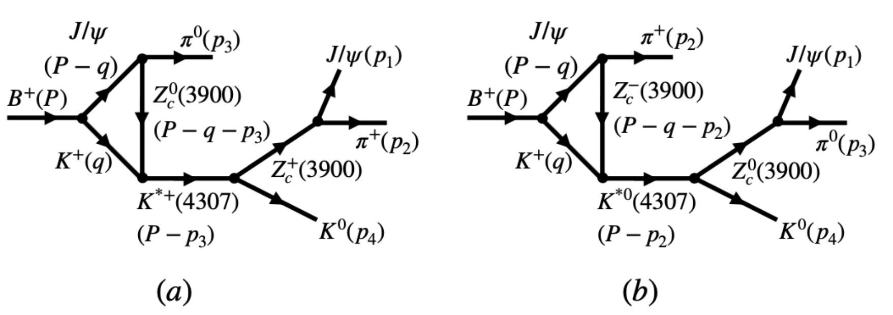
The decay process $B^{+}\to J/\psi\pi^{+}\pi^{0}K^{0}$ proceeding through $K^{*}(4307)$ formation can be visualized diagrammatically as shown in Fig. 1, where the interaction between a $K^{+}$ and a $Z^{0\,(-)}_{c}(3900)$ generates the $K^{*+\,(0)}(4307)$ Ren:2018pcd, which decays to $J/\psi\pi^{+\,(0)}K^{0}$. The nature of $Z_{c}(3900)$ is still under debate. Here, as done in Ref. Ren:2018pcd, we follow the model of Ref. Aceti:2014uea where the state is generated from the interaction between $D\bar{D}^{*}$ and $J/\psi\pi$ within coupled channels as a weakly bound state of the $D\bar{D}^{*}$ system, with a finite width from its decay to the $J/\psi\pi$ channel.

Due to the nature of $K^{*}(4307)$ and $Z_{c}(3900)$, the weak vertex $B^{+}\to J/\psi K^{+}$ is the most favored for forming $Z_{c}(3900)$ and $K^{*}(4307)$. At the quark level, it involves internal emission of a $W^{+}$ via $\bar{b}\to\bar{c}$ ($W^{+}\to c\bar{s})$ transitions, which are both Cabibbo favored (see Fig. 2).

Based on the quantum chromodynamics factorization approach for non-leptonic $B$-meson decays Beneke:2000ry, the amplitude related to the weak vertex shown in Fig. 2 can be written as

$\displaystyle t_{B^{+}\to J/\psi K^{+}}=\frac{G_{F}}{\sqrt{2}}V_{cb}V^{*}_{cs}a_{2}\langle J/\psi|(\bar{c}c)_{V}|0\rangle\langle K|(\bar{b}s)_{V}|B\rangle,$

(1)

where $G_{F}$ is the Fermi coupling constant, $V_{cb}$, $V^{*}_{cs}$ are elements of the Cabibbo-Kobayashi-Maskawa matrix, $a_{2}$ is an effective coupling constant, $\langle J/\psi|(\bar{c}c)_{V}|0\rangle$ is the factorized amplitude for the production of a $J/\psi$ via the vector current $\bar{c}\gamma_{\mu}c$ and $\langle K|(\bar{b}s)_{V}|B\rangle$ represents the transition matrix element $B^{+}\to K^{+}$. The amplitude $\langle J/\psi|(\bar{c}c)_{V}|0\rangle$ can be parametrized in terms of the decay constant $f_{J/\psi}$, the mass $m_{J/\psi}$ and the polarization vector $\epsilon_{J/\psi\,\mu}$ of the $J/\psi$ vector meson as Neubert:1997uc

$\displaystyle\langle J/\psi|(\bar{c}c)_{V}|0\rangle=\epsilon_{J/\psi\,\mu}m_{J/\psi}f_{J/\psi},$

(2)

while the transition matrix element $B^{+}(p)\to K^{+}(p^{\prime})$ can be written as Neubert:1997uc

$\displaystyle\langle K^{+}(p^{\prime})|(\bar{b}s)_{V}|B^{+}(p)\rangle=\left[(p+p^{\prime})_{\mu}-\frac{m^{2}_{B^{+}}-m^{2}_{K^{+}}}{Q^{2}}Q_{\mu}\right]F_{1}(Q^{2})+\frac{m^{2}_{B^{+}}-m^{2}_{K^{+}}}{Q^{2}}Q_{\mu}F_{0}(Q^{2}).$

(3)

In Eq. (3), $Q_{\mu}=(p-p^{\prime})_{\mu}$, $F_{1}(Q^{2})$ and $F_{0}(Q^{2})$ correspond to form factors, which satisfy the condition $F_{1}(0)=F_{0}(0)$ Neubert:1997uc, and $m_{B^{+}}$ ($m_{K^{+}}$) is the mass of the $B^{+}$ ($K^{+}$) meson. The $Q^{2}$ dependence of these form factors can be written as Deandrea:1993ma

$\displaystyle F_{i}(Q^{2})=\frac{F_{i}(0)}{1-Q^{2}/m^{2}_{P\,i}},$

(4)

with $i=0,1$, $m_{P\,i}$ being the mass of the lowest lying meson with the appropriate quantum numbers, i.e., $J^{P}=0^{+}$ for $F_{0}$ ($m_{P}=5890$ MeV) and $1^{-}$ for $F_{1}$ ($m_{P}=5430$ MeV), and

$\displaystyle F_{1}(0)=F_{0}(0)=0.49\pm 0.12.$

(5)

Using Eq. (1), we can determine the branching ratio for the process $B^{+}\to J/\psi K^{+}$ as

$\displaystyle\text{Br}(B^{+}\to J/\psi K^{+})=\frac{|\vec{p}_{\text{CM}}|}{8\pi\Gamma_{B^{+}}m^{2}_{B^{+}}}\sum_{\lambda}|t_{B^{+}\to J/\psi K^{+}}|^{2},$

(6)

where the symbol $\sum\limits_{\lambda}$ indicates sum over the polarizations of $J/\psi$, $|\vec{p}_{\text{CM}}|$ is the center of mass momentum of the $J/\psi K^{+}$ system, $\Gamma_{B^{+}}$ is the width of the $B^{+}$ meson and, from Eqs. (1) and (3)

	$\displaystyle\sum_{\lambda}|t_{B^{+}\to J/\psi K^{+}}|^{2}$	$\displaystyle=\frac{G^{2}_{F}}{2}|V_{cb}|^{2}|V_{cs}|^{2}|a_{2}|^{2}m^{2}_{J/\psi}f^{2}_{J/\psi}F^{2}_{1}(Q^{2})$
		$\displaystyle\quad\times\left[-(p+p^{\prime})^{2}+\frac{(m^{2}_{B^{+}}-m^{2}_{K^{+}})^{2}}{m^{2}_{J/\psi}}\right].$		(7)

Considering $a_{2}=0.21\pm 0.02$ Neubert:1997uc, $G_{F}=1.166\times 10^{-11}$ MeV^-2, $|V_{cs}|=0.977\pm 0.017$, $|V_{cb}|=(42.2\pm 0.8)\times 10^{-3}$, $m_{J/\psi}=3096.9\pm 0.006$ MeV, $\Gamma_{B^{+}}=(4.01839\pm 0.0098)\times 10^{-10}$ MeV Tanabashi:2018oca, and $f_{J/\psi}=405\pm 14$ MeV Neubert:1997uc, we get

$\displaystyle\text{Br}(B^{+}\to J/\psi K^{+})\simeq(0.83\pm 0.32)\times 10^{-3},$

(8)

which is compatible with the measured branching ratio of Tanabashi:2018oca

$\displaystyle\text{Br}(B^{+}\to J/\psi K^{+})_{\text{measured}}=(1.01\pm 0.028)\times 10^{-3}.$

(9)

Based on the above discussion, the dominant contribution from the weak vertex in the processes depicted in Fig. 1, can be written, for convenience, as

$\displaystyle t_{B^{+}\to J/\psi K^{+}}=C_{B^{+}\to J/\psi K^{+}}(P+q)\cdot\epsilon_{J/\psi}(P-q),$

(10)

where $P^{\mu}$ ($q^{\mu}$) is the four-momentum of the $B^{+}$ ($K^{+}$), and the coefficient $C_{B^{+}\to J/\psi K^{+}}$, which corresponds to $\frac{G_{F}}{\sqrt{2}}|V_{cb}||V_{cs}||a_{2}|m_{J/\psi}f_{J/\psi}F_{1}$ of Eq. (7), is fixed to reproduce the observed branching ratio, i.e., Eq. (9), to be more in agreement with the experimental finding,

$\displaystyle C_{B^{+}\to J/\psi K^{+}}=(7.16\pm 0.11)\times 10^{-8}.$

(11)

Since $Z_{c}(3900)$ and $K^{*}(4307)$ couple to $J/\psi\pi$ and $KZ_{c}(3900)$, respectively, in s-wave Aceti:2014uea; Ren:2018pcd, we can introduce the coupling constants $g_{Z_{c}\to J/\psi\pi}$ and $g_{K^{*}\to KZ_{c}}$ to describe the contribution from these vertices in Fig. 1. Such contribution can be expressed in terms of the contraction $\epsilon\cdot\epsilon^{\prime}$ between the polarization vectors of the particles involved, $Z_{c}(3900)$ and $J/\psi$ or $K^{*}(4307)$ and $Z_{c}(3900)$, and the corresponding coupling constant, obtained from Refs. Aceti:2014uea; Ren:2018pcd. In this way, using the Feynman rules, the amplitudes associated with the diagrams in Fig. 1 are given by

	$\displaystyle-it_{\mathcal{A}}$	$\displaystyle=C_{\mathcal{A}}\frac{1}{s_{3(\mathcal{A})}-m^{2}_{K^{*}(\mathcal{A})}+i\Gamma_{K^{*}(\mathcal{A})}m_{K^{*}(\mathcal{A})}}\frac{1}{s_{2(\mathcal{A})}-m^{2}_{Z_{\mathcal{A}}}+i\Gamma_{Z(\mathcal{A})}m_{Z(\mathcal{A})}}$
		$\displaystyle\quad\times\Bigg[F_{-}\Bigg\{P_{\sigma}-\frac{(P-p_{\mathcal{A}})_{\sigma}}{M^{2}_{Z(\mathcal{A})}}(P^{2}-p_{\mathcal{A}}\cdot P)\Bigg\}I^{(0\mathcal{A})}+\left\{F_{+}+\frac{F_{-}}{M^{2}_{Z(\mathcal{A})}}\left(P^{2}-p_{\mathcal{A}}\cdot P\right)\right\}I^{(1\mathcal{A})}_{\sigma}$
		$\displaystyle\quad\quad\quad+\frac{(P-p_{\mathcal{A}})_{\sigma}}{M^{2}_{Z(\mathcal{A})}}\times\left\{F_{+}p^{\mu}_{\mathcal{A}}-2\frac{P^{2}}{m^{2}_{J/\psi}}P^{\mu}\right\}I^{(1\mathcal{A})}_{\mu}+\Bigg\{\frac{P_{\sigma}}{m^{2}_{J/\psi}}+\frac{(P-p_{\mathcal{A}})_{\sigma}}{M^{2}_{Z(\mathcal{A})}}$
		$\displaystyle\quad\quad\quad\times\left(1+\frac{p_{\mathcal{A}}\cdot P}{m^{2}_{J/\psi}}\right)\Bigg\}I^{(2\mathcal{A})}-\frac{1}{M^{2}_{Z(\mathcal{A})}}\Bigg\{F_{+}p^{\mu}_{\mathcal{A}}-2\frac{P^{2}}{m^{2}_{J/\psi}}P^{\mu}\Bigg\}I^{(2\mathcal{A})}_{\sigma\mu}$
		$\displaystyle\quad\quad\quad+\frac{(P-p_{\mathcal{A}})_{\sigma}}{M^{2}_{Z(\mathcal{A})}}\frac{(-p^{\mu}_{\mathcal{A}}+2P^{\mu})}{m^{2}_{J/\psi}}I^{(3\mathcal{A})}_{\mu}-\Bigg\{\frac{1}{m^{2}_{J/\psi}}+\frac{1}{M^{2}_{Z(\mathcal{A})}}\left(1+\frac{p_{\mathcal{A}}\cdot P}{m^{2}_{J/\psi}}\right)\Bigg\}I^{(3\mathcal{A})}_{\sigma}$
		$\displaystyle\quad\quad\quad-\frac{1}{M^{2}_{Z(\mathcal{A})}m^{2}_{J/\psi}}\Bigg\{(P-p_{\mathcal{A}})_{\sigma}I^{(4\mathcal{A})}+(-p^{\mu}_{\mathcal{A}}+2P^{\mu})I^{(4\mathcal{A})}_{\sigma\mu}-I^{(5\mathcal{A})}_{\sigma}\Bigg\}\Bigg]$
		$\displaystyle\quad\times\left[-g^{\sigma\rho}+\frac{(P-p_{\mathcal{A}})^{\sigma}(P-p_{\mathcal{A}})^{\rho}}{m^{2}_{K^{*}(\mathcal{A})}}\right]\left[-g_{\rho\beta}+\frac{(p_{1}+p_{2})_{\rho}p_{2\beta}}{m^{2}_{Z(\mathcal{A})}}\right]\epsilon^{\beta}_{J/\psi}(p_{1}),$		(12)

where the subscript $\mathcal{A}$ refers to the diagrams $(a)$ and $(b)$ in Fig. 1, with $s_{3(\mathcal{A})}=s_{124}=(p_{1}+p_{2}+p_{4})^{2}$ [$s_{134}=(p_{1}+p_{3}+p_{4})^{2}$], $s_{2(\mathcal{A})}=s_{12}=(p_{1}+p_{2})^{2}$ [$s_{13}=(p_{1}+p_{3})^{2}$], $p_{\mathcal{A}}=p_{3}$ ($p_{2}$), $m_{Z(\mathcal{A})}=m_{Z^{+}_{c}}$ ($m_{Z^{0}_{c}}$), $M_{Z(\mathcal{A})}=m_{Z^{0}_{c}}$ ($m_{Z^{-}_{c}}$) is the mass of the $Z_{c}$ particle involved in the triangular loops, $m_{K^{*}(\mathcal{A})}=m_{K^{*+}(4307)}$ [$m_{K^{*0}(4307)}$], $\Gamma_{Z(\mathcal{A})}=\Gamma_{Z^{+}_{c}}$ ($\Gamma_{Z^{0}_{c}}$), $\Gamma_{K^{*}(\mathcal{A})}=\Gamma_{K^{*+}(4307)}$ [$\Gamma_{K^{*0}(4307)}$] for the diagram $(a)$ [$(b)$]. In Eq. (12),

$\displaystyle F_{\pm}=1\pm\frac{P^{2}}{m^{2}_{J/\psi}},$

(13)

and the constant $C_{\mathcal{A}}$ corresponds to a product of the coupling constants involved in the different vertices shown in Fig. 1. To be more exact,

$\displaystyle C_{a}=-C_{b}=\frac{\sqrt{2}}{3}C_{B^{+}\to J/\psi K^{+}}g^{2}_{Z_{c}\to J/\psi\pi}g^{2}_{K^{*}\to KZ_{c}},$

(14)

where $g_{Z_{c}\to J/\psi\pi}$ is the coupling constant of $Z_{c}(3900)$ to the $J/\psi\pi$ system in isospin 1, and whose value is obtained from the model of Ref. Aceti:2014uea, and $g_{K^{*}\to KZ_{c}}$ represents the coupling of $K^{*}(4307)$ to a $KZ_{c}(3900)$ system in isospin $1/2$, which can be found from the model of Ref. Ren:2018pcd. The values used here are $g_{Z_{c}\to J/\psi\pi}=3715$ MeV and $g_{K^{*}\to KZ_{c}}=22143$ MeV Ren:2019umd. The phase convention $|\pi^{+}>=-|I=1,I_{3}=1\rangle$, $|K^{-}\rangle=-|I=1/2,I_{3}=-1/2\rangle$ has been used in our calculations.

In Eq. (12), $I^{(0\mathcal{A})}$, $I^{(1\mathcal{A})}_{\alpha}$, $I^{(2\mathcal{A})}_{\alpha\beta}$, $I^{(3\mathcal{A})}_{\alpha}$, $I^{(4\mathcal{A})}_{\alpha\beta}$ and $I^{(5\mathcal{A})}_{\alpha}$ are integrals defined as

	$\displaystyle I^{(0\mathcal{A})}$	$\displaystyle=\int\frac{d^{4}q}{(2\pi)^{4}}\frac{1}{\mathcal{D}(q,p_{\mathcal{A}})},\quad I^{(1\mathcal{A})}_{\alpha}=\int\frac{d^{4}q}{(2\pi)^{4}}\frac{q_{\alpha}}{\mathcal{D}(q,p_{\mathcal{A}})},\quad I^{(2\mathcal{A})}_{\alpha\beta}=\int\frac{d^{4}q}{(2\pi)^{4}}\frac{q_{\alpha}q_{\beta}}{\mathcal{D}(q,p_{\mathcal{A}})},$
	$\displaystyle I^{(3\mathcal{A})}_{\alpha}$	$\displaystyle=\int\frac{d^{4}q}{(2\pi)^{4}}\frac{q^{2}q_{\alpha}}{\mathcal{D}(q,p_{\mathcal{A}})},\quad I^{(4\mathcal{A})}_{\alpha\beta}=\int\frac{d^{4}q}{(2\pi)^{4}}\frac{q^{2}q_{\alpha}q_{\beta}}{\mathcal{D}(q,p_{\mathcal{A}})},\quad I^{(5\mathcal{A})}_{\alpha}=\int\frac{d^{4}q}{(2\pi)^{4}}\frac{q^{4}q_{\alpha}}{\mathcal{D}(q,p_{\mathcal{A}})},$		(15)

where

$\displaystyle\mathcal{D}(q,p_{\mathcal{A}})=[(P-q)^{2}-m^{2}_{J/\psi}+i\epsilon][q^{2}-m^{2}_{K^{+}}+i\epsilon][(P-p_{\mathcal{A}}-q)^{2}-M^{2}_{Z(\mathcal{A})}+i\epsilon].$

(16)

The integrals $I^{(2\mathcal{A})}$ and $I^{(4\mathcal{A})}$ in Eq. (12) correspond to the contraction of the metric tensor $g^{\alpha\beta}$ with the integrals $I^{(2\mathcal{A})}_{\alpha\beta}$ and $I^{(4\mathcal{A})}_{\alpha\beta}$ of Eq. (15), respectively. The integrals in Eq. (15) are regularized by using a cut-off of $\sim 700$ MeV for the center of mass momentum of the $K-Z_{c}$ system, which is compatible with the cut-off used in Ref. Ren:2018pcd to generate the $K^{*}(4307)$ from the $KD\bar{D}^{*}$ system. For more details on the calculation of the integrals in Eq. (15) we refer the reader to the Appendix A.

Using the amplitude in Eq. (12), the decay width $\Gamma$ for the process $B^{+}(P)\to J/\psi(p_{1})\pi^{+}(p_{2})\pi^{0}(p_{3})K^{0}(p_{4})$ can be obtained as

	$\displaystyle\Gamma$	$\displaystyle=\frac{1}{2m_{B^{+}}}\int\frac{d^{3}p_{1}}{(2\pi)^{3}2E_{1}(\vec{p}_{1})}\int\frac{d^{3}p_{2}}{(2\pi)^{3}2E_{2}(\vec{p}_{2})}\int\frac{d^{3}p_{3}}{(2\pi)^{3}2E_{3}(\vec{p}_{3})}\int\frac{d^{3}p_{4}}{(2\pi)^{3}2E_{4}(\vec{p}_{4})}$
		$\displaystyle\quad\quad\quad\quad\quad\times(2\pi)^{4}\delta^{(4)}(P-p_{1}-p_{2}-p_{3}-p_{4})\sum_{\lambda}|t_{a}+t_{b}|^{2}.$		(17)

Using the $\delta$-function of Eq. (17), and the relations

	$\displaystyle s_{124}$	$\displaystyle=(p_{1}+p_{2}+p_{4})^{2}=(P-p_{3})^{2}=m^{2}_{B^{+}}+m^{2}_{3}-2m_{B^{+}}E_{3},$
	$\displaystyle s_{134}$	$\displaystyle=(p_{1}+p_{3}+p_{4})^{2}=(P-p_{2})^{2}=m^{2}_{B^{+}}+m^{2}_{2}-2m_{B^{+}}E_{2},$		(18)

with $E_{2}=\sqrt{\vec{p}^{\,2}_{2}+m^{2}_{2}}$ ($E_{3}=\sqrt{\vec{p}^{\,2}_{3}+m^{2}_{3}}$) being the energy related to the particle with three-momentum $\vec{p}_{2}$ ($\vec{p}_{3}$) and mass $m_{2}$ ($m_{3}$) in the rest frame of the decaying particle, we can write Eq. (17) as

	$\displaystyle\Gamma$	$\displaystyle=\frac{1}{(2\pi)^{7}2^{6}m^{3}_{B^{+}}}\int\limits_{s^{\text{min}}_{124}}^{s^{\text{max}}_{124}}ds_{124}\int\limits_{s^{\text{min}}_{134}}^{s^{\text{max}}_{134}}ds_{134}\int\limits_{E^{\text{min}}_{1}}^{E^{\text{max}}_{1}}dE_{1}\int\limits_{0}^{2\pi}d\phi_{1}\int\limits_{-1}^{1}d\text{cos}\theta_{3}\int\limits_{0}^{2\pi}d\phi_{3}$
		$\displaystyle\quad\times\frac{|\vec{p}_{2}||\vec{p}_{3}|}{|\vec{p}_{2}+\vec{p}_{3}|}\Theta(1-\text{cos}^{2}\theta_{1})\Theta(m_{B^{+}}-E_{1}-E_{2}-E_{3})\sum_{\lambda}|t_{a}+t_{b}|^{2}.$		(19)

To arrive to Eq. (19) we have considered, without lost of generality, that particle 2 is along the $z$-axis, and we integrate on the solid angle of particles 1 and 3. The value $\text{cos}\theta_{1}$, with $\theta_{1}$ being the angle between the vectors $\vec{p}_{1}$ and $\vec{p}_{2}+\vec{p}_{3}$, is fixed by the $\delta$-function of Eq. (17),

$\displaystyle\text{cos}\theta_{1}=\frac{(m_{B^{+}}-E_{1}-E_{2}-E_{3})^{2}-\vec{p}^{\,2}_{1}-m^{2}_{4}-(\vec{p}_{2}+\vec{p}_{3})^{2}}{2|\vec{p}_{1}||\vec{p}_{2}+\vec{p}_{3}|}.$

(20)

The related Heaviside $\Theta$-function in Eq. (19) guaranties that $|\text{cos}\theta_{1}|\leqslant 1$, as it should be. In this way, if $(\theta_{23},\phi_{23})$ are the polar and azimutal angles, respectively, that the vector $\vec{p}_{2}+\vec{p}_{3}$ forms with the axes we can obtained $\vec{p}_{1}$ as

$\displaystyle\vec{p}_{1}=R_{z}(\phi_{23})R_{y}(\theta_{23})|\vec{p}_{1}|\left(\begin{array}[]{c}\text{sin}\theta_{1}\text{cos}\phi_{1}\\ \text{sin}\theta_{1}\text{sin}\phi_{1}\\ \text{cos}\theta_{1}\end{array}\right),$

where $\text{sin}\theta_{1}=+\sqrt{1-\text{cos}^{2}\theta_{1}}$, $|\vec{p}_{1}|=\sqrt{E^{2}_{1}-m^{2}_{1}}$, $R_{y}$ and $Rz$ represent rotation matrices around the $y$ and $z$ axis, respectively,

$\displaystyle R_{y}(\theta_{23})=\left(\begin{array}[]{ccc}\text{cos}\theta_{23}&0&\text{sin}\theta_{23}\\ 0&1&0\\ -\text{sin}\theta_{23}&0&\text{cos}\theta_{23}\end{array}\right),\quad R_{z}(\phi_{23})=\left(\begin{array}[]{ccc}\text{cos}\phi_{23}&-\text{sin}\phi_{23}&0\\ \text{sin}\phi_{23}&\text{cos}\phi_{23}&0\\ 0&0&1\end{array}\right).$

The angles $\theta_{23}$ and $\phi_{23}$ can be obtained in terms of the components $x$, $y$ and $z$ of the vectors $\vec{p}_{2}$ and $\vec{p}_{3}$, which are given by

$\displaystyle\vec{p}_{2}=|\vec{p}_{2}|\left(\begin{array}[]{c}0\\ 0\\ 1\end{array}\right),\quad\vec{p}_{3}=|\vec{p}_{3}|\left(\begin{array}[]{c}\text{sin}\theta_{3}\text{cos}\phi_{3}\\ \text{sin}\theta_{3}\text{sin}\phi_{3}\\ \text{cos}\theta_{3}\end{array}\right),$

as

	$\displaystyle\text{cos}\theta_{23}=\frac{p_{2z}+p_{3z}}{|\vec{p}_{2}+\vec{p}_{3}|},$	$\displaystyle\quad\text{sin}\theta_{23}=+\sqrt{1-\text{cos}^{2}\theta_{23}},$		(36)
	$\displaystyle\text{cos}\phi_{23}=\frac{p_{2x}+p_{3x}}{|\vec{p}_{2}+\vec{p}_{3}|\text{sin}\theta_{23}},$	$\displaystyle\quad\text{sin}\phi_{23}=\frac{p_{2y}+p_{3y}}{|\vec{p}_{2}+\vec{p}_{3}|\text{sin}\theta_{23}}.$		(37)

Note that $|\vec{p}_{2}|=\sqrt{E^{2}_{2}-m^{2}_{2}}$ and $|\vec{p}_{3}|=\sqrt{E^{2}_{3}-m^{2}_{3}}$ are related to the invariant masses $s_{134}$ and $s_{124}$ through Eq. (18). The momentum $\vec{p}_{4}$ can be obtained as $\vec{p}_{4}=-\vec{p}_{1}-\vec{p}_{2}-\vec{p}_{3}$. In this way, the last ingredient to determine Eq. (17) is the limits of the integrals, which are

	$\displaystyle s^{\text{min}}_{124}$	$\displaystyle=(m_{1}+m_{2}+m_{4})^{2},\quad s^{\text{max}}_{124}=(m_{B^{+}}-m_{3})^{2},$		(38)
	$\displaystyle s^{\text{min}}_{134}$	$\displaystyle=(m_{1}+m_{3}+m_{4})^{2},\quad s^{\text{max}}_{134}=(m_{B^{+}}-m_{2})^{2},$		(39)
	$\displaystyle E^{\text{min}}_{1}$	$\displaystyle=m_{1},\quad E^{\text{max}}_{1}=\frac{m^{2}_{B^{+}}+m^{2}_{1}-s^{\text{min}}_{234}}{2m_{B^{+}}},\quad s^{\text{min}}_{234}=(m_{2}+m_{3}+m_{4})^{2}.$		(40)

From Eq. (19), we can determine the corresponding $J/\psi\pi K$ invariant mass distribution as

	$\displaystyle\frac{d\Gamma}{ds_{124}}$	$\displaystyle=\frac{1}{(2\pi)^{7}2^{6}m^{3}_{B^{+}}}\int\limits_{s^{\text{min}}_{134}}^{s^{\text{max}}_{134}}ds_{134}\int\limits_{E^{\text{min}}_{1}}^{E^{\text{max}}_{1}}dE_{1}\int\limits_{0}^{2\pi}d\phi_{1}\int\limits_{-1}^{1}d\text{cos}\theta_{3}\int\limits_{0}^{2\pi}d\phi_{3}$
		$\displaystyle\quad\times\frac{|\vec{p}_{2}||\vec{p}_{3}|}{|\vec{p}_{2}+\vec{p}_{3}|}\Theta(1-\text{cos}^{2}\theta_{1})\Theta(m_{B^{+}}-E_{1}-E_{2}-E_{3})\sum_{\lambda}|t_{a}+t_{b}|^{2},$		(41)
	$\displaystyle\frac{d\Gamma}{ds_{134}}$	$\displaystyle=\frac{1}{(2\pi)^{7}2^{6}m^{3}_{B^{+}}}\int\limits_{s^{\text{min}}_{124}}^{s^{\text{max}}_{124}}ds_{124}\int\limits_{E^{\text{min}}_{1}}^{E^{\text{max}}_{1}}dE_{1}\int\limits_{0}^{2\pi}d\phi_{1}\int\limits_{-1}^{1}d\text{cos}\theta_{3}\int\limits_{0}^{2\pi}d\phi_{3}$
		$\displaystyle\quad\times\frac{|\vec{p}_{2}||\vec{p}_{3}|}{|\vec{p}_{2}+\vec{p}_{3}|}\Theta(1-\text{cos}^{2}\theta_{1})\Theta(m_{B^{+}}-E_{1}-E_{2}-E_{3})\sum_{\lambda}|t_{a}+t_{b}|^{2}.$		(42)

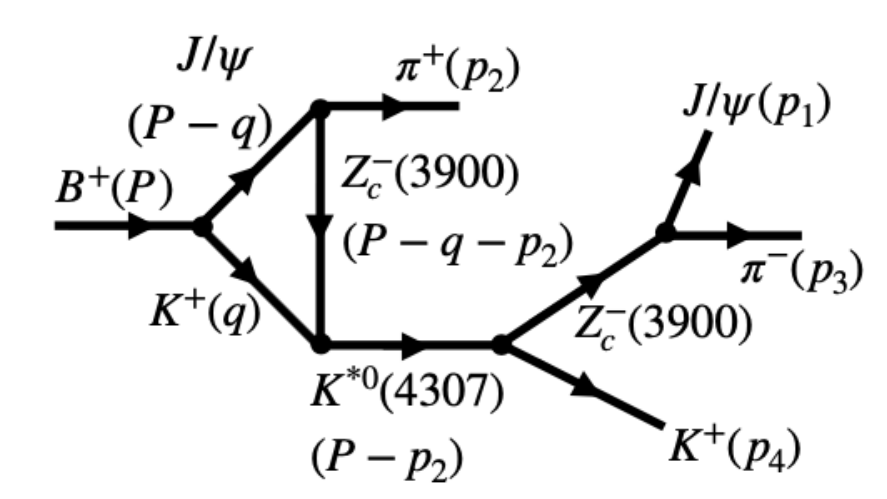
As we mentioned in the introduction, the decay $B^{+}\to J/\psi\pi^{+}\pi^{-}K^{+}$ has been used for the experimental investigation of the properties of $X(3872)$. In this reaction, the reconstruction of the $J/\psi\pi^{-}K^{+}$ invariant mass distribution, can also serve to investigate the properties of $K^{*}(4307)$. For the process $B^{+}\to J/\psi\pi^{+}\pi^{-}K^{+}$, as can be seen in Fig. 3, the formation of $K^{*}(4307)$ is completely analogous to the one shown in Fig. 1(b), with the exception that the vertices $K^{*0}(4307)\to Z^{0}_{c}(3900)K^{0}\to J/\psi\pi^{0}K^{0}$ should be replaced by $K^{*0}(4307)\to Z^{-}_{c}(3900)K^{+}\to J/\psi\pi^{-}K^{+}$. This makes that the product of the coupling constants $g_{K^{*0}(4307)\to Z^{0}_{c}(3900)}g_{K^{0}Z^{0}_{c}\to J/\psi\pi^{0}}$ appearing in the amplitude related to the diagram in Fig. 1(b) should be substituted by $g_{K^{*0}(4307)\to K^{+}Z^{-}_{c}(3900)}g_{Z^{-}_{c}\to J/\psi\pi^{-}}$, which, by using the corresponding Clebsch-Gordan coefficients, is $\sqrt{2}$ times bigger than the former product. In this way, the calculation of the decay width for $B^{+}\to J/\psi\pi^{+}\pi^{-}K^{+}$ and the determination of the $J/\psi\pi^{-}K^{+}$ invariant mass distribution is completely analogous to the one for the reaction $B^{+}\to J/\psi\pi^{+}\pi^{0}K^{0}$, but we have now contribution from only one Feynman diagram instead of two (see Fig. 3) and the couplings, as explained above, are different.