Milky Way Satellite Census. II. Galaxy–Halo Connection Constraints Including the Impact of the Large Magellanic Cloud Astropy (Astropy Collaboration et al. 2013), ChainConsumer (Hinton 2016), emcee (Foreman-Mackey et al. 2013), Healpy (healpy.readthedocs.io), Pandas (McKinney 2010), Scikit-Learn (Pedregosa et al. 2011), IPython (Pérez & Granger 2007), Jupyter (jupyter.org), Matplotlib (Hunter 2007), NumPy (van der Walt et al. 2011), SciPy (Jones et al. 2001), Seaborn (seaborn.pydata.org).
Abstract
The population of Milky Way (MW) satellites contains the faintest known galaxies and thus provides essential insight into galaxy formation and dark matter microphysics. Here we combine a model of the galaxy–halo connection with newly derived observational selection functions based on searches for satellites in photometric surveys over nearly the entire high Galactic latitude sky. In particular, we use cosmological zoom-in simulations of MW-like halos that include realistic Large Magellanic Cloud (LMC) analogs to fit the position-dependent MW satellite luminosity function. We report decisive evidence for the statistical impact of the LMC on the MW satellite population due to an estimated observed LMC-associated satellites, consistent with the number of LMC satellites inferred from Gaia proper-motion measurements, confirming the predictions of cold dark matter models for the existence of satellites within satellite halos. Moreover, we infer that the LMC fell into the MW within the last at high confidence. Based on our detailed full-sky modeling, we find that the faintest observed satellites inhabit halos with peak virial masses below at confidence, and we place the first robust constraints on the fraction of halos that host galaxies in this regime. We predict that the faintest detectable satellites occupy halos with peak virial masses above , highlighting the potential for powerful galaxy formation and dark matter constraints from future dwarf galaxy searches.
DES-2019-0491 \reportnumFERMILAB-PUB-19-606-AE
I Introduction
The sample of confirmed and candidate Milky Way (MW) satellite galaxies has more than doubled in the last years. Modern imaging surveys have driven these discoveries; in particular, following the successes of the Sloan Digital Sky Survey (SDSS) in the early s (Willman et al. 2005a; Willman et al. 2005b; Belokurov et al. 2006; Belokurov et al. 2007; Belokurov et al. 2008; Belokurov et al. 2009; Belokurov et al. 2010; Grillmair 2006; Grillmair 2009; Sakamoto & Hasegawa 2006; Zucker et al. 2006; Irwin et al. 2007; Walsh et al. 2007), the Dark Energy Survey (DES) and the Panoramic Survey Telescope and Rapid Response System Pan-STARRS1 (PS1) have discovered and three new satellite galaxy candidates, respectively (Bechtol et al. 2015; Drlica-Wagner et al. 2015; Kim & Jerjen 2015; Koposov et al. 2015; Laevens et al. 2015a; Laevens et al. 2015b; Luque et al. 2016). These systems are identified as arcminute-scale overdensities of individually resolved stars, and many have already been spectroscopically confirmed. Meanwhile, other surveys with the Dark Energy Camera and VST ATLAS have recently discovered several additional satellites (Martin et al. 2015; Drlica-Wagner et al. 2016; Torrealba et al. 2016a; Torrealba et al. 2016b; Torrealba et al. 2018; Koposov et al. 2018; Mau et al. 2020).
Nonetheless, the current census of MW satellites is likely highly incomplete, particularly for faint systems in the outer regions of the MW halo. This is evidenced by the detection of three new ultrafaint satellites in the first of Hyper Suprime-Cam Strategic Survey Program (HSC-SSP) imaging data (Homma et al. 2016; Homma et al. 2018; Homma et al. 2019) and by the discovery of Antlia II, the lowest surface brightness galaxy currently known, using RR Lyrae member stars identified in Gaia DR2 (Torrealba et al. 2019). In the near future, the Legacy Survey of Space and Time (LSST) conducted from the Vera C. Rubin Observatory will be able to detect satellites over the entire southern sky down to a surface brightness of (Ivezić et al. 2008; Tollerud et al. 2008; Hargis et al. 2014; Nadler et al. 2019b).
Interpreting the cosmological and astrophysical implications of these discoveries requires a detailed understanding of the observational selection effects for each survey under consideration. In a companion paper (Drlica-Wagner et al. 2020, hereafter 36), we derive observational selection functions for DES and PS1 based on searches for simulated satellites in each dataset. These selection functions encode the probability that satellites in either survey are detectable as a function of their absolute magnitude, heliocentric distance, physical size, and position on the sky. They incorporate realistic photometric error models, selection masks that exclude highly reddened regions near the Galactic disk, and the influence of local stellar density on satellite detectability. Detection sensitivity is linked to sky position because various surveys have imaged different parts of the sky at varying depths, and accurately modeling this effect is crucial in order to disentangle anisotropy in the underlying MW satellite system from selection effects.
In this paper, we combine the observational selection functions derived in 36 with a detailed model of the galaxy–halo connection and high-resolution cosmological zoom-in simulations of MW-mass host halos to infer the position-dependent MW satellite luminosity function. Although several empirical models have recently been used to study subsets of the MW satellite population (Jethwa et al. 2018; Kim et al. 2018; Newton et al. 2018; Nadler et al. 2019b), this is the first analysis that is directly based on imaging data over more than ; indeed, our analysis covers of the high Galactic latitude sky. Moreover, our galaxy–halo connection model allows us to marginalize over astrophysical uncertainties in our fit to the observed DES and PS1 satellite populations. We quantify the impact of the largest MW satellite, the Large Magellanic Cloud (LMC), and its associated satellites on the observed DES and PS1 satellite populations. We find that the satellites accreted with a realistic LMC analog—defined in terms of its mass, heliocentric distance, and infall time—are essential to fit the DES and PS1 luminosity functions simultaneously; this finding constitutes a remarkable confirmation of hierarchical structure formation. We predict that () of the known satellites observed by DES (PS1) fell into the MW with the LMC, consistent with the number of LMC-associated satellites inferred from Gaia proper-motion measurements (Kallivayalil et al. 2018; Patel et al. 2020).
Our analysis constrains the properties of the lowest-mass halos that host observed satellites, which we infer to have peak virial masses below at confidence. This finding, along with constraints on the faint-end slope of the luminosity function, can be used to inform feedback prescriptions in hydrodynamic simulations (Sawala et al. 2016b; Fitts et al. 2018; Simpson et al. 2018; Munshi et al. 2019; Wheeler et al. 2019). Constraints on the minimum halo mass also hold broad implications for the microphysical properties of dark matter (e.g., Drlica-Wagner et al. 2019; Nadler et al. 2019a). Crucially, our model can be extended to explore the degeneracies between baryonic physics and deviations from the cold dark matter (CDM) paradigm.
This paper is organized as follows. We first provide an overview of our framework in Section II. We then describe the simulations (Section III), galaxy–halo connection model (Section IV), observational selection functions (Section V), and statistical framework (Section VI) used in our analysis. We present our results in Section VII, focusing on the observed DES and PS1 satellite populations (§VII.1), the impact of the LMC system (§VII.2), the total MW satellite population (§VII.3), galaxy–halo connection model constraints (§VII.4), the properties of halos that host the faintest observed satellites (§VII.5), and the implications of our findings for dark matter microphysics (§VII.6). We discuss the main theoretical uncertainties in our analysis in Section VIII, and we conclude in Section IX. Appendices provide additional details on our galaxy–halo connection model (Appendix A) and statistical framework (Appendix B), the robustness of our results to observational systematics (Appendix C) and resolution effects (Appendix D), and the observed DES and PS1 satellite populations (Appendix E).
Throughout, we use the term “galaxy–halo connection model” to refer to a model that describes how the properties of galaxies, including luminosity and size, are related to the properties of halos, such as peak virial mass. Furthermore, “log” refers to the base- logarithm.
II Analysis Overview
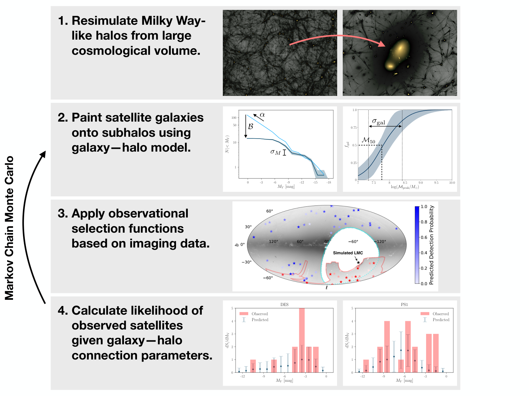
Using the observed population of MW satellites to constrain our galaxy–halo connection model requires the following ingredients (see Figure 1 for a visualization of each step).
- 1.
A model that predicts the underlying MW satellite population.
- 2.
An observational selection function that, convolved with the prediction in the previous step, yields a prediction for the observed satellite population.
- 3.
A model for the likelihood of producing the true MW satellite population given the prediction from the previous step.
The first step above can either be performed using either a hydrodynamic simulation, in which galaxy formation is modeled at the simulation level, or an empirical prescription for painting galaxies onto halos. We take the latter approach in this paper, which allows for a more flexible modeling framework, as well as the use of simulations that are closer approximations to the MW system. Indeed, our results may help to constrain feedback prescriptions in hydrodynamic simulations. Note that the assumed dark matter model (e.g., cold vs. warm dark matter or collisionless vs. interacting dark matter) affects the underlying satellite population and often manifests as a cutoff in the abundance of halos—and thus faint galaxies—below a halo mass threshold determined by the microphysical properties of dark matter.
The steps outlined above each rely on tools that have been developed in previous studies and in 36. Here we simply provide a brief description of each step, and we defer additional details to the Appendices.
III Simulations
III.1 General Description
Our model of the underlying MW satellite population is built on high-resolution dark matter–only zoom-in simulations of MW-mass host halos selected from the suite of hosts presented in Mao et al. 2015, which have virial masses between and .11 1 We define virial quantities according to the Bryan–Norman virial overdensity (Bryan & Norman 1998), with as appropriate for the cosmological parameters adopted in our zoom-in simulations: , , , and (Mao et al. 2015). The highest-resolution particles in these simulations have a mass of , and the softening length in the highest-resolution regions is .
Halo catalogs and merger trees were generated using the Rockstar halo finder and the consistent-trees merger code (Behroozi et al. 2013b; Behroozi et al. 2013c). Subhalos in these simulations are well resolved down to a present-day maximum circular velocity of (Mao et al. 2015). To be conservative, we only use subhalos with both and peak maximum circular velocity . In Appendix D, we show that these resolution thresholds are sufficient for modeling the satellite populations of interest here.
III.2 Host Halo and LMC Analog Selection
The MW might be atypical compared to the average halos of a similar mass (e.g., Boylan-Kolchin et al. 2010; Busha et al. 2011; Rodríguez-Puebla et al. 2013; Fielder et al. 2019); in particular, its satellite population is likely affected by the existence of the LMC system and the “satellites of satellites” that accreted with the LMC into the virial radius of the MW (Lynden-Bell 1976; D’Onghia & Lake 2008; Lu et al. 2016; Dooley et al. 2017). In addition, the detailed merger history of the MW—such as the early accretion of an LMC-mass galaxy inferred from Gaia data—might affect its faint satellite population (Bose et al. 2019).
Thus, we select MW-like host halos that each have an LMC analog with realistic internal and orbital properties; both of these hosts experience an early major merger similar to the Gaia-Enceladus accretion event (see Appendix A.3 for details). We define realistic LMC analogs as subhalos with
- 1.
present-day maximum circular velocity ,
- 2.
present-day heliocentric distance , and
- 3.
time of accretion onto the MW less than ago.
These criteria yield two MW-like host halos with virial masses of and , respectively. Both of these hosts were used in the less restrictive host halo set defined in Nadler et al. 2019b, and both have a Navarro–Frenk–White (NFW) concentration parameter that is consistent with constraints set using the combination of satellite and globular cluster dynamics measured by Gaia (Callingham et al. 2019; Watkins et al. 2019). The LMC analogs in these two simulations have present-day virial masses of and respectively, and both have peak virial masses of . These LMC analogs accreted onto their host halos and ago, respectively, and their orbital dynamics are consistent with LMC proper-motion measurements (e.g., Kallivayalil et al. 2013).
Our fiducial LMC analogs have masses that are consistent with LMC mass estimates based on stellar stream dynamics, satellite dynamics, and the orbital histories of both Magellanic Clouds (Besla 2015; Peñarrubia et al. 2016; Erkal & Belokurov 2019; Erkal et al. 2019).22 2 Although detailed exploration of Magellanic Cloud binary systems is beyond the scope of this work, we note that Shao et al. 2018 and Cautun et al. 2019a found that LMC analogs with SMC-like companions are typically more massive than isolated LMC analogs. However, different studies have adopted various definitions of “LMC mass,” and precision in the LMC mass definition (and particularly in the distinction between peak and present-day halo mass) is crucial going forward. We expect that our inference is most sensitive to the peak mass rather than the present-day mass of the LMC because peak mass correlates more directly with the expected abundance of LMC satellites, particularly for recent infall scenarios. Other probes of LMC mass are likely sensitive to these quantities in different ways, and some—including timing arguments (e.g., Peñarrubia et al. 2016) and orbit-rewinding to infer LMC satellite abundances (e.g., Patel et al. 2020)—might be most sensitive to the ratio of the LMC and MW halo masses.
Although the masses of our host halos are consistent with observational constraints for the MW (e.g., Busha et al. 2011; Bland-Hawthorn & Gerhard 2016; Patel et al. 2017), our simulations span a narrower range of host mass relative to the uncertainty on this quantity inferred from Gaia measurements. For example, Callingham et al. 2019 found that the MW host virial mass lies between and at the confidence level (also see Cautun et al. 2019b; Li et al. 2019b; Li et al. 2019a). Since subhalo abundance is proportional to host halo mass, predicted satellite abundances scale linearly with MW mass, modulo second-order changes in subhalo disruption due to variations in the mass accretion history of the central galaxy (Kelley et al. 2019; Samuel et al. 2020). Ideally, our analysis would be performed using MW-like host halos—all of which include realistic LMC analogs—that bracket the current range of allowed MW host mass; however, the availability of such MW-like systems is limited by the statistics of our simulations. Thus, we do not marginalize over the full range of allowed MW host masses in this work. We estimate the potential impact of this uncertainty in Appendix A.1.
IV Galaxy–Halo Connection Model
To associate satellite galaxies with subhalos in the simulations described above, we use a modified version of the model developed in Nadler et al. 2019b. This model parameterizes the relationship between satellite and subhalo properties and the effects of baryonic physics on subhalo populations in flexible ways, which allows us to marginalize over the relevant theoretical uncertainties. Additional model details and tests are presented in Appendix A.
IV.1 Satellite Luminosities
To associate satellite luminosities with subhalos, we follow Nadler et al. 2019b by employing an abundance-matching procedure that monotonically relates the absolute -band magnitude of satellites, , to the peak circular velocity of subhalos, .33 3 We perform abundance matching using to incorporate the effects of halo assembly bias and to mitigate the impact of subhalo tidal stripping (Reddick et al. 2013; Lehmann et al. 2017). This relation is constrained by the GAMA survey (Loveday et al. 2015; Geha et al. 2017) for bright systems () and is extrapolated into the regime of dim satellites by treating the faint-end slope of the satellite luminosity function, , and the lognormal scatter in luminosity at fixed , as free parameters. We assume that this scatter is lognormal and constant as a function of halo properties in our fiducial analysis; we explore a mass-dependent scatter model in Appendix A.2.
Our abundance-matching model is a simple, empirical prescription for assigning satellite luminosities that is not designed to capture the complexities of star formation in ultrafaint dwarf galaxies. For example, Bose et al. 2018 argued that star formation in systems dimmer than is effectively shut down by reionization, resulting in two distinct galaxy populations today. While our abundance-matching model is consistent with the current data, which are fit fairly well by a single power-law luminosity function (see 36), it will be valuable to investigate more detailed models of stellar mass growth and to compare against a wider range of observables, including the inferred star formation histories of MW satellites, in future work.
IV.2 Satellite Sizes
We assign physical sizes to satellites by extrapolating a modified version of the size–virial radius relation from Kravtsov 2013, which links a galaxy’s stellar 3D half-mass radius to its halo’s virial radius, into the faint satellite regime. In particular, we set the mean predicted size of each satellite at accretion according to
| (1) |
where and are free parameters, denotes the subhalo virial radius measured at accretion, and is a normalization constant. Following Nadler et al. 2019b, we equate the 3D half-mass radii predicted by Equation 1 to azimuthally averaged projected half-light radii; this conversion neglects mass-to-light weighting and projection effects. Nonetheless, this size relation yields reasonable mean sizes when compared to the observed population of classical and SDSS-discovered satellites (Nadler et al. 2019b).
We draw the size of each satellite from a lognormal distribution with a mean given by Equation 1 and a standard deviation of , which is a free parameter in our model. When fitting the observed satellite populations, we only compare predicted and mock satellites with in order to exclude likely star clusters from the analysis. We explore a more conservative cut of in Appendix C.2.
The size prescription described above assumes that satellite sizes are fixed after accretion onto the MW. However, post-infall effects such as tidal stripping and tidal heating can shrink or enlarge satellites depending on their orbital histories (Peñarrubia et al. 2009; Errani et al. 2015; Fattahi et al. 2018). In Appendix A.4, we show that our key results are not sensitive to these effects using a simple model for satellite size evolution due to tidal stripping.
IV.3 Subhalo Disruption Due to Baryonic Effects
To incorporate the effects of baryonic physics—and particularly the tidal influence of the Galactic disk—on our simulated subhalo populations, we apply a random forest algorithm trained on hydrodynamic simulations to predict the probability that each subhalo will be disrupted in a hydrodynamic resimulation based on its orbital and internal properties (Garrison-Kimmel et al. 2017b; Nadler et al. 2018). We model the strength of this disruption effect using the free parameter , which is defined such that corresponds to fiducial hydrodynamic predictions (Nadler et al. 2018) and larger (smaller) values of correspond to more effective (less effective) subhalo disruption. For each subhalo, we set
| (2) |
where is the fiducial disruption probability returned by the machine-learning algorithm in Nadler et al. 2018.
IV.4 Galaxy Formation Efficiency
The stochastic, nonlinear nature of galaxy formation in low-mass halos likely leads to a smoothly varying fraction of occupied halos, rather than a sharp cutoff in the efficiency of galaxy formation (Sawala et al. 2016b; Fitts et al. 2018; Munshi et al. 2019; Wheeler et al. 2019). Thus, in our fiducial model, we parameterize the fraction of halos that host galaxies of any mass, referred to as the galaxy occupation fraction, following Graus et al. 2019,
| (3) |
where is the largest virial mass a subhalo ever attains, which typically occurs before infall into the MW; is the peak halo mass at which of halos host galaxies of any mass; and is the width of the galaxy occupation fraction. In our fiducial model, and are free parameters. Note that in the limit , this reduces to a model in which all halos with host a galaxy.
Although our analysis does not constrain , Equation 3 is a simple, physically motivated form of the occupation fraction that will be interesting to explore in future work. Note that we parameterize the occupation fraction in terms of peak halo mass (rather than, e.g., ) because is more easily interpretable and connects directly to constraints on alternative dark matter models (e.g., Nadler et al. 2019a).
IV.5 Orphan Satellites
Because we model faint galaxies that can potentially inhabit subhalos near the resolution limit of our simulations, it is important to account for artificially disrupted subhalos that might host “orphan” satellites (Guo et al. 2011, and see Bose et al. 2019 for a recent example of the importance of orphans in satellite modeling). To model orphans, we follow the prescription in Nadler et al. 2019b, which identifies disrupted subhalos in each simulation, interpolates their orbits to using a softened gravitational force law and a dynamical friction model, and accounts for tidal stripping with a mass-loss model calibrated on high-resolution test simulations. We parameterize the effective abundance of orphans by setting their disruption probabilities equal to
| (4) |
where is the final scale factor at which each subhalo enters the virial radius of the MW, and is a parameter that captures deviations from disruption probabilities in hydrodynamic simulations, which are well fit by (Nadler et al. 2019b). Thus, larger (smaller) values of correspond to a greater (smaller) contribution from orphan satellites.
Following Nadler et al. 2019b, we include orphan satellites by fixing in our fiducial model. Thus, we effectively assume that subhalo disruption in dark matter–only simulations is a numerical artifact (van den Bosch & Ogiya 2018; van den Bosch et al. 2018) but that subhalo disruption in hydrodynamic simulations is a physical effect. We show that our results are largely insensitive to the value of in Appendix A.6.
V Observational Selection Functions
We employ the DES and PS1 survey selection functions derived in 36, which have been publicly distributed as machine-learning classifiers that predict satellite detection probability given absolute magnitude, ; heliocentric distance, ; azimuthally averaged projected half-light radius, ; and sky position.44 4 The DES Y3A2 and PS1 DR1 selection functions are publicly available at https://github.com/des-science/mw-sats. The predicted detection probabilities are derived from searches for simulated satellites in catalog-level DES and PS1 data, and they employ geometric cuts that restrict observable satellites to lie within the respective survey footprint and that mask regions where satellite detection is challenging due to interstellar extinction, bright nearby stars, and bright extragalactic objects.
We self-consistently apply these position-dependent detection criteria to our predicted satellite populations by matching the on-sky position of our LMC analogs to the true on-sky position of the LMC. In particular, we choose random observer locations from the halo center, and we perform appropriate rotations to our subhalo populations for each observer location to match the true LMC position. We apply the DES selection function for satellites within the overlap region of the two surveys, and we only count satellites within a fiducial heliocentric distance of .
VI Statistical Framework
To fit our galaxy–halo model to the DES and PS1 luminosity functions derived in 36, we generate predicted satellite populations given a set of galaxy–halo connection model parameters, , by performing mock DES-plus-PS1 surveys using the selection functions described above. For each host halo and each realization of our satellite model, we bin mock-observed satellites according to their absolute magnitude. We further split satellites in each absolute magnitude bin into high () and low () surface brightness samples to incorporate satellite size information in our fit.55 5 In particular, we calculate the effective surface brightness averaged within the half-light radius as , where is measured in units of . We list the DES and PS1 satellites used in this analysis in Table 3.
Next, we calculate the number of predicted satellites in each bin via
| (5) |
where indexes the satellites in bin , is the detection probability returned by the appropriate observational selection function, is the disruption probability due to baryonic effects (Equation 2), and is the galaxy occupation fraction (Equation 3). For objects that lie in the overlap region of the DES and PS1 footprints, we calculate using the DES selection function.
We note that detection probability mainly depends on surface brightness and present-day heliocentric distance (see 36), disruption probability mainly depends on orbital properties (Nadler et al. 2018), and galaxy occupation depends on according to Equation 3. Thus, our model for satellite detectability is coupled to our galaxy occupation fraction model, since surface brightness is directly linked to due to our abundance-matching assumption. Nonetheless, our results are largely unaffected if we exclude the galaxy occupation fraction from our model, confirming that can be interpreted as the probability that a halo hosts a satellite brighter than , corresponding to the faintest satellite in our observational sample.
We assume that satellites populate each bin in absolute magnitude–surface brightness parameter space according to an independent Poisson point process with a rate parameter that depends on absolute magnitude, surface brightness, and our galaxy–halo connection model parameters. Because our model yields noisy estimates of , we marginalize over its range of possible values in each bin, following Nadler et al. 2019b. The likelihood of observing the set of DES and PS1 satellites, and (specified by their absolute magnitudes and surface brightnesses), given a set of model parameters is then
| (6) |
where () is the observed number of DES (PS1) satellites in bin , and () is a vector of the number of mock DES (PS1) satellites in bin from several realizations of our model at fixed . These realizations include draws over host halos, observer locations, and our galaxy–halo connection model, which is stochastic at fixed . Note that steps 1–3 in Figure 1 generate mock satellite populations and , and step 4 compares these to the observed populations and . The explicit forms of and are given in Equation B1.
Finally, we use Bayes’s theorem to compute the posterior distribution over galaxy–halo connection model parameters,
| (7) |
where is our prior on the galaxy–halo connection model parameters (given in Appendix B.2), is the Bayesian evidence, and is given by Equation 6. To sample from this posterior, we run iterations of the Markov Chain Monte Carlo (MCMC) sampler emcee (Foreman-Mackey et al. 2013) to sample the eight free parameters using walkers. We discard a burn-in period of autocorrelation lengths, corresponding to steps, which leaves more than independent samples.
VII Results
We now present our results, focusing on the observed DES and PS1 satellite populations (§VII.1), the impact of the LMC system (§VII.2), the total MW satellite population (§VII.3), the galaxy–halo connection model constraints (§VII.4), the properties of the halos that host faint satellites (§VII.5), and the implications for dark matter microphysics (§VII.6).
VII.1 Observed Satellite Populations
Figure 2 shows the and confidence intervals for the observed DES and PS1 satellite luminosity functions given by draws from the posterior of our fiducial model, which is consistent with both datasets. We note that the DES and PS1 likelihoods individually yield consistent results.
Figure 3 shows the corresponding satellite size distributions drawn from our fiducial posterior. Our model is consistent with the sizes of both the observed DES and PS1 satellites. It very slightly overpredicts the sizes of observed DES systems; however, we reiterate that our size model does not allow for size reduction due to tidal stripping or size enlargement due to tidal heating, which affect satellites with close pericentric passages to the Galactic disk (e.g., Amorisco 2019). Our findings in Appendix A.4 suggest that the post-infall size evolution of satellites in subhalos with and does not significantly affect our inference.
Our fiducial model is consistent with the outer radial distributions of both DES and PS1 satellites, but it slightly underpredicts the number of satellites near the center of the MW (), particularly in PS1. We explore this minor discrepancy in Appendix A.3, where we show that our galaxy–halo connection model constraints and inferred total MW satellite population are largely unaffected if the radial distribution is forced to match the data.
VII.2 The Impact of the LMC
To assess the impact of the LMC and its satellites on the MW satellite population, we test the following models in addition to our fiducial model, which includes a realistic, recently accreted LMC system by construction.
- 1.
No LMC: a model with four host halos that have the same mean concentration as our fiducial hosts but no LMC analog.
- 2.
Misplaced LMC: a model with our fiducial host halos in which subhalo positions are reflected, effectively placing the DES footprint in the northern hemisphere.
- 3.
Early LMC Infall: a model with two host halos that have the same mean concentration as our fiducial hosts with LMC analogs that pass our LMC and heliocentric distance cuts but fall into the MW and ago, respectively.
For each alternative LMC scenario listed above, we refit the observed DES and PS1 satellite populations, sampling over the same eight parameters used in our fiducial analysis.
Our fiducial model is favored over the No LMC, Misplaced LMC, and Early LMC Infall scenarios with Bayes factors of , , and , respectively. In addition, both host halos in the Early LMC Infall case are individually disfavored with Bayes factors of . Thus, we find decisive statistical evidence for the impact of the LMC on the MW satellite population, particularly within and near the DES footprint. Moreover, we infer that the LMC system fell into the MW within the last at high confidence. We also note that, in our fiducial host with more massive MW and LMC halos, the LMC reaches pericenter near the second-to-last simulation snapshot (i.e., ago). Performing our analysis using the final snapshot for this host noticeably degrades the fit due to the dispersal and disruption of LMC satellites during the LMC’s pericentric passage. Thus, we use the second-to-last snapshot for this host in our fiducial analysis, and we remark that satellite abundances can potentially constrain the number of allowed pericentric passages for the LMC.
The alternative LMC scenarios defined above are strongly disfavored relative to our fiducial model because they cannot produce a sufficient number of dim satellites in the DES footprint without overpredicting the number of observed PS1 satellites. This is a direct consequence of the spatial overdensity of subhalos near the LMC analogs in our fiducial simulations; in particular, the projected density of resolved subhalos within of the LMC on the sky is enhanced by relative to the density on a random patch of sky.
To quantify the number of satellites in our fiducial model that are associated with the LMC, we explore the following definitions of LMC-associated subhalos.
- 1.
Fiducial definition. A subhalo is associated with the LMC if it is within the virial radius of the LMC halo at the time of LMC infall into the MW.
- 2.
Gravitationally influenced definition. A subhalo is associated with the LMC if it has ever passed within the virial radius of the LMC halo.
Here LMC infall is defined as the snapshot at which the center of the LMC halo crosses within the MW virial radius. Note that nearly all systems that satisfy our strict definition are bound to the LMC at the time of LMC infall.
Under the fiducial (gravitationally influenced) definitions above, we predict that () total LMC-associated subhalos (above our cuts of and ) exist within the virial radius of the MW today, where the confidence interval is estimated by drawing from our fiducial posterior. We predict that () of these subhalos form galaxies with and (in agreement with an earlier estimate by Jethwa et al. 2018), and that () of these satellites survive tidal disruption due to the Galactic disk. Of these surviving LMC-associated satellites, we predict that () are currently observed by DES and that () are currently observed by PS1.
Our statistical probe of LMC satellite association is remarkably consistent with the number of observed LMC satellites inferred from Gaia proper-motion measurements, which indicate that four galaxies in or near the DES footprint—excluding the Small Magellanic Cloud (SMC)—are associated with the LMC, and that two satellites in or near the PS1 footprint are potentially associated with the LMC (Kallivayalil et al. 2018; Patel et al. 2020).66 6 A recent analysis based on Gaia proper-motion measurements and hydrodynamic simulations suggests that two bright satellites in or near DES, Fornax and Carina, may also be LMC-associated (Pardy et al. 2020; however, see Patel et al. 2020). In addition, the orbital dynamics of our predicted LMC satellites are consistent with Gaia proper-motion measurements for these likely LMC-associated systems. These predictions are also consistent with other empirical models (Deason et al. 2015; Jethwa et al. 2016; Dooley et al. 2017; Sales et al. 2017; Kallivayalil et al. 2018; Erkal & Belokurov 2019; Zhang et al. 2019) and with hydrodynamic simulations of isolated LMC analogs (Jahn et al. 2019).
In Appendix D, we show that the properties of our LMC-like systems are not significantly affected by the realizations of small-scale power in our fiducial simulations. However, we caution that the number of predicted LMC satellites observed by DES and PS1 depends on the particular properties of our two LMC analogs. Thus, exploring the robustness of these results using a suite of zoom-in simulations selected to contain realistic LMC systems with a range of internal and orbital properties is an important avenue for future work.

VII.3 The Total MW Satellite Population
Figure 4 shows the total MW satellite luminosity function and surface brightness distribution resulting from our fit to the DES and PS1 satellite populations. We infer that a total of satellites with and exist within the virial radius of the MW, where uncertainties correspond to confidence intervals calculated by sampling from our fiducial posterior. Thus, we predict that satellites remain undiscovered in a standard CDM scenario, roughly one-fourth of which are associated with the LMC. This is larger than the fraction of satellites that have ever fallen into the MW that are associated with the LMC because our fiducial LMC analogs accreted recently, making their satellites less likely to be disrupted. Our prediction for the total number of MW satellites is consistent with several recent studies (Jethwa et al. 2018; Kim et al. 2018; Newton et al. 2018; Nadler et al. 2019b), and it is lower than the empirical estimate in 36, which was recognized to be inflated due to the assumption of an isotropic satellite distribution. This prediction will be tested by upcoming deep imaging surveys; indeed, HSC-SSP has already started to probe this population of distant, low surface brightness MW satellites by discovering three new ultrafaint satellite candidates in of imaging data (Homma et al. 2016; Homma et al. 2018; Homma et al. 2019).
To estimate whether our predictions are consistent with HSC-SSP observations, we draw realizations of the MW satellite population from our fiducial posterior and calculate the number of systems within the DES or PS1 footprints that would not be observed by the appropriate survey. We then estimate the number of these systems currently observed by an HSC-like survey covering that detects all satellites (i.e., systems with and ) down to a surface brightness of and out to a heliocentric distance of , assuming an isotropic satellite distribution at high Galactic latitudes and accounting for subhalo disruption. There are six known satellites in the HSC footprint, but two of the six (Sextans and Leo IV) are detected at high significance in PS1 by at least one of the search algorithms in 36. We find that our mock HSC survey detects satellites, which is in slight tension with the number of systems detected by HSC (four, after discounting Sextans and Leo IV).
| Parameter | Physical Interpretation | Confidence Interval |
|---|---|---|
| Faint-end Slope | Power-law slope of satellite luminosity function | |
| Luminosity scatter | Scatter in luminosity at fixed | |
| occupation mass | Mass at which of halos host galaxies | |
| Baryonic effects | Strength of subhalo disruption due to baryons | |
| Occupation scatter | Scatter in galaxy occupation fraction | |
| Size amplitude | Amplitude of galaxy–halo size relation | |
| Size scatter | Scatter in half-light radius at fixed halo size | |
| Size power-law index | Power-law index of galaxy–halo size relation | |
Note. — Asterisks mark prior-driven constraints.
Figure 4 illustrates several predictions from hydrodynamic simulations of isolated and satellite dwarf galaxies. Our results are largely consistent with the luminosity function of bright MW satellites in hydrodynamic simulations of the Local Group using the Feedback In Realistic Environments (FIRE) feedback prescription, down to the FIRE resolution limit of (Garrison-Kimmel et al. 2019). Note that these FIRE simulations do not include LMC or SMC analogs, which accounts for the discrepancy with both our predictions and the observed luminosity function at . Interestingly, other recent hydrodynamic simulations indicate that different star formation prescriptions significantly impact the amplitude and faint-end slope of the luminosity function for satellites of isolated LMC-like halos (Munshi et al. 2019). Thus, our constraints on the faint-end slope, which are driven by satellites with (corresponding to stellar mass ), can be used to inform subgrid star formation prescriptions.
VII.4 Galaxy–Halo Connection Model Constraints
The posterior distribution for our fiducial model is shown in Figure 5, and the corresponding galaxy–halo connection model constraints are listed in Table 1. Note that we obtain statistically consistent results when fitting the DES and PS1 satellite populations with either of our two fiducial simulations individually in terms of both the Bayesian evidence and the galaxy–halo connection model constraints. In particular, no parameter constraints shift by more than relative to the fiducial values reported below when the fit is performed using either simulation individually. We now discuss each constraint in detail.
- 1.
The inferred faint-end slope of the satellite luminosity function is steeper than that reported in a previous study based on classical and SDSS satellites (Nadler et al. 2019b). Our constraint is consistent with the faint-end slope derived from higher-luminosity field galaxies in the GAMA survey (Loveday et al. 2015; Wright et al. 2017), even though it is based on a sample that extends nearly fainter than that used in GAMA. We note that is the most sensitive parameter in our analysis to modeling assumptions and details of the observed satellite population.
- 2.
The scatter in luminosity at fixed is constrained to at confidence, which may inform hydrodynamic feedback prescriptions that predict a steep increase in luminosity scatter at low masses (e.g., see Wechsler & Tinker 2018). Our lack of a lower limit on is consistent with previous studies of faint galaxy samples (e.g., Lehmann et al. 2017). Meanwhile, large values of are not allowed because too many low- satellites upscatter to observable luminosities, resulting in overpredicted luminosity functions. To confirm that this upper limit is robust, we calculate Bayes factors by drawing samples from the posterior in bins of , finding that () is disfavored relative to with a Bayes factor of ().77 7 We provide details on our Bayes factor calculations in Appendix B.3. These upper limits are comparable to the scatter typically inferred from abundance-matching analyses of brighter systems () and smaller than that from hydrodynamic simulations of dwarf galaxies (e.g., Rey et al. 2019); however, we caution that our constraint might be impacted by the use of only two independent realizations of the MW satellite population. In addition, it is potentially misleading to compare global constraints on scatter to those derived from the MW alone. Both of these caveats are important to explore in future work.
- 3.
The peak mass at which of halos host galaxies is inferred to be less than at confidence. Note that this summary statistic depends on the lower limit of our prior on , since the posterior flattens near its lower limit, which is chosen based on the resolution of our simulations. Thus, we also calculate Bayes factors by drawing from the posterior in bins of to confirm that this summary statistic is robust. We find that () is disfavored relative to arbitrarily low values of with a Bayes factor of (). The current data are not able to place a lower limit on , which would correspond to the detection of a cutoff in galaxy formation.
- 4.
Our posterior is consistent with , corresponding to our fiducial baryonic disruption model. Although a large spread in disruption strength is allowed by the data, extremely efficient () and inefficient () subhalo disruption relative to hydrodynamic simulations is strongly disfavored. These constraints widen when our lognormal prior on is relaxed; however, zero subhalo disruption (corresponding to ) is robustly ruled out.
- 5.
The scatter in the galaxy occupation fraction is consistent with zero, which makes sense given our lack of a lower limit on . Models with large scatter in the occupation fraction (), corresponding to extremely stochastic galaxy formation, are disfavored relative to a step function occupation fraction at confidence. Note that the slope of the posterior is driven by the lower limit of our prior; as this limit decreases, the posterior flattens.
- 6.
The amplitude of the galaxy–halo size relation, defined as the typical size of a satellite in a halo with at accretion, is constrained to lie between and at confidence. For larger values of , satellites are too large to be detected with high probability, and the DES and PS1 luminosity functions are underpredicted; for smaller values of , many predicted satellites do not pass our cut, and the luminosity functions are underpredicted.
- 7.
The scatter in the galaxy–halo size relation is constrained to lie between and at confidence. For larger values of , faint satellites upscatter to large sizes too frequently, which results in underpredicted luminosity functions. Our confidence lower limit on of is consistent with the value estimated in Kravtsov 2013. Lower values of lead to slightly too many predicted DES and PS1 satellites; however, our results are consistent with at confidence.
- 8.
The power-law index of the galaxy–halo size relation is constrained to lie between and at confidence. For shallower power-law slopes, satellite sizes do not change appreciably as a function of halo size, which results in a worse joint fit to the observed absolute magnitude and surface brightness distribution. We note that the posterior widens when our Gaussian prior on is relaxed.
VII.5 Properties of Halos that Host the Faintest Satellites
We now explore the properties of the lowest-mass halos inferred to host MW satellites. The left panel of Figure 6 shows the galaxy occupation fraction derived from our statistical inference, where uncertainties are estimated by drawing from our fiducial posterior. By sampling from our fiducial posterior, we infer that halos with a peak virial mass below and peak circular velocity below host at least one of the faintest observed satellites. To convert these into maximally conservative upper limits, we account for the uncertainty in MW host halo mass using the procedure described in Appendix A.1, which yields limits on the minimum halo mass and peak circular velocity of and at confidence. Furthermore, we predict that the faintest observed satellite inhabits a halo with , on average.88 8 The faintest observed satellite in our analysis, Cetus II, is detected by DES with (Drlica-Wagner et al. 2015; Table 3).
These results improve upon the minimum halo mass constraint derived from classical and SDSS satellites (Nadler et al. 2019b) by a factor of , and they are consistent with the constraints reported in Jethwa et al. 2018. Moreover, these upper limits are not in significant tension with the expected atomic cooling limit of , contrary to recent studies based on the radial MW satellite distribution (e.g., Graus et al. 2019) and consistent with the findings in Bose et al. 2019.
We caution that the median galaxy occupation fraction shown in Figure 6 is driven by the assumed functional form in Equation 3 and is therefore arbitrary. Although the functional form in Equation 3 is consistent with results from hydrodynamic simulations for , this particular functional form is not required to fit the DES and PS1 luminosity functions. Rather, we have evidence that above a peak virial mass of . To verify that the assumed form of the galaxy occupation fraction does not impact our constraints, we also test a binned model in which we fit for and a corresponding occupation mass. We find that the resulting and occupation constraints are consistent with those inferred from our fiducial analysis.
A wide range of galaxy occupation fractions have been reported in hydrodynamic simulations, with some placing as high as (Sawala et al. 2016b; Fitts et al. 2018). However, recent hydrodynamic simulations run at higher resolution result in efficient galaxy formation in significantly lower-mass halos, and some claim that all halos down to the resolution limit consistently host star particles (Wheeler et al. 2019). In addition, simulations of galaxy formation at early pre-reionization epochs show that stellar systems form in halos with masses as low as (e.g., see Fig. 13 in Côté et al. 2018 for a compilation of recent simulation results). Most recently, high-resolution simulations of high-redshift galaxy formation that include the effects of spatially and temporally inhomogeneous reionization find (Katz et al. 2020).
Our galaxy occupation fraction constraint implies that models with are in significant tension with the observed MW satellite population, as long as MW satellite formation is representative of galaxy formation at this halo mass scale, on average. This assumption may not be true if the reionization history of the MW’s Lagrangian volume differs from the average reionization history of an MW-mass halo hosting dwarf galaxies of the masses considered here (however, see Alvarez et al. 2009; Busha et al. 2010). Note that analyses based on H I surveys of Local Group dwarfs indicate a suppression mass scale similar to our constraint (Tollerud & Peek 2018).
Due to our abundance-matching assumption, the lowest-mass halos in our model host the faintest galaxies, on average. Thus, our constraints on the masses of these halos are conservative, since the most massive halos in our simulations are forced to host more easily observable satellites at fixed distance and size, modulo baryonic disruption effects and abundance-matching scatter. In other words, our abundance-matching model yields a testable prediction: the faintest galaxies should inhabit the halos with the lowest pre-infall virial masses. We expect this correlation to be weakened by post-infall effects, including tidal stripping, but we can nevertheless infer the present-day joint distribution of halo mass and satellite luminosity or stellar mass. We illustrate this stellar mass–halo mass (SMHM) relation in the right panel of Figure 6. Our inferred SMHM relation is generally consistent with recent results (e.g., Jethwa et al. 2018). Like the faint-end slope of the luminosity function, the SMHM relation can be used to discriminate between different subgrid models of star formation and stellar feedback (Munshi et al. 2019). As in previous studies, we find that the SMHM relation in the ultrafaint regime falls off more steeply than extrapolations of abundance-matching relations derived using higher-mass field galaxies (Behroozi et al. 2013a). Interestingly, Agertz et al. 2020 found that full on-the-fly radiative transfer is necessary to match the steepness and normalization of our inferred SMHM relation for a fixed hydrodynamic feedback prescription.
Ultimately, our predictions must be confronted with the dynamical mass function of observed satellites, measurements of which will improve significantly in the era of upcoming spectroscopic facilities and giant segmented mirror telescopes (Simon et al. 2019). A preliminary comparison of our joint predicted distribution of luminosity and with the measured stellar velocity dispersions of DES and PS1 satellites suggests that our model is consistent with the inferred central densities of low-luminosity satellites (). Although there is a systematic discrepancy between observed and predicted values of for brighter systems (the “too big to fail” problem), our simple comparison does not account for the conversion from line-of-sight velocity dispersion measured within observed half-light radii to or the tidal effects of the Galactic disk on the density profiles of surviving subhalos. Moreover, the systems for which predicted densities are higher than those inferred observationally are susceptible to baryonic feedback processes that core the inner regions of halos (Di Cintio et al. 2014), and this effect has been shown to alleviate the too big to fail problem (Brooks et al. 2013; Sawala et al. 2016a; Wetzel et al. 2016; Lovell et al. 2017; Garrison-Kimmel et al. 2019).
Finally, we explore the properties of the halos inferred to host the faintest potentially detectable galaxies. In particular, we calculate the minimum peak halo mass necessary for halos to contain a stellar population of at least , chosen to represent the approximate threshold for which it would be possible to observationally confirm a stellar system as a dark matter--dominated dwarf galaxy.99 9 For many MW satellites, this will likely require spectroscopy with giant segmented mirror telescopes (Simon et al. 2019). By populating a higher-resolution version of one of our fiducial simulations and sampling from the posterior of our abundance-matching relation, we find that systems at the observational threshold occupy halos with at confidence. To detect even lower-mass halos, gravitational probes of dark matter that are independent of baryonic content, e.g. gravitational lensing or stellar streams, must be employed.
VII.6 Implications for Dark Matter Microphysics
Many deviations from CDM lead to a cutoff in the abundance of low-mass halos. Several authors have used MW satellite abundances to constrain a free-streaming cutoff induced by warm dark matter (e.g., Macciò & Fontanot 2010; Kennedy et al. 2014; Lovell et al. 2014; Jethwa et al. 2018). Nadler et al. 2019a showed that similar constraints apply to other dark matter models, resulting in limits on the velocity-independent scattering cross section between dark matter and baryons. Our statistical detection of halos with peak virial masses below therefore translates directly into constraints on various microphysical properties of dark matter.
Nadler et al. 2019a found that the minimum halo mass inferred in this fashion is comparable to the limit on the half-mode mass , which corresponds to the scale at which the matter power spectrum is suppressed by a critical amount relative to CDM due to dark matter free streaming or interactions. Performing a statistical inference in which the half-mode mass is varied will constrain it to lie below our upper limit on , since the abundance of halos at and above the half-mode mass is reduced relative to CDM.
Thus, for a simple and conservative estimate of the dark matter constraints resulting from our analysis, we set the upper limit on equal to our upper limit on the minimum halo mass, i.e., , which corresponds to a lower limit on the half-mode scale of . Using the relations in Nadler et al. 2019a with the cosmological parameters and corresponding to the simulations used in our analysis (see Section III.1), this yields a lower limit of on the mass of thermal relic warm dark matter and an upper limit of on the velocity-independent dark matter–baryon scattering cross section for a dark matter particle mass, both at confidence. We leave a detailed investigation of dark matter constraints to future work.
VIII Theoretical Uncertainties
We aim to present a thorough galaxy–halo connection model that allows us to marginalize over the most important theoretical uncertainties when modeling the MW satellite population. Nonetheless, our modeling choices necessarily affect the predicted number of detected low-mass halos and thus our upper limit on the minimum halo mass, . In this section, we briefly discuss the main uncertainties in this analysis and their impact on our constraint.
To do so, we consider the upper limit on as a function of modeling assumptions, starting with the most conservative model possible and adding one assumption at a time. We illustrate the results of this exercise in Figure 7 for upper limits calculated as follows.
- 1.
Minimal CDM. Assuming a maximally massive MW halo given Gaia constraints (i.e., a virial mass of ; Callingham et al. 2019; Cautun et al. 2019b; Li et al. 2019b; Li et al. 2019a), count the subhalos within the virial radius of the MW in order of decreasing until the number of kinematically confirmed DES and PS1 satellites is matched, and set the lowest corresponding value of equal to the upper limit on .
- 2.
MW Host Mass. Repeat the previous step with the MW host mass fixed to its average value in our two fiducial simulations (i.e., an average virial mass of ).
- 3.
Subhalo Disruption. Repeat the previous step many times with the subhalo number weighted by disruption probability, sampling from our fiducial posterior, to calculate an upper limit on at confidence.
- 4.
Satellites (confirmed). Repeat the previous step including the observational detection probabilities for mock satellites in the DES and PS1 footprints by drawing satellite properties from our fiducial posterior.
- 5.
Satellites (unconfirmed). Repeat the previous step including the unconfirmed candidate satellites detected by DES and PS1 in the observed tally.
This yields for models (i)–(v), respectively. Note that models (i)–(iii) are extremely conservative, since subhalos are counted in order of decreasing ; however, these models do not reproduce the observed position-dependent MW satellite luminosity function or radial distribution. Model (iv) yields the conservative limit presented in Appendix C.1, and model (v) yields our fiducial constraint, uncorrected for MW host halo mass. Although we have not explicitly considered artificial subhalo disruption in this list of theoretical uncertainties (e.g., van den Bosch & Ogiya 2018; van den Bosch et al. 2018), our fiducial orphan satellite model effectively assumes that subhalo disruption in dark matter–only simulations is entirely artificial, which is a conservative choice.
Figure 7 shows that both fitting the satellite luminosity function and including the population of faint, kinematically unconfirmed satellite galaxies in our fit yield significant increases in constraining power. We emphasize that our galaxy–halo connection model is conservative from the perspective of upper limits on the minimum halo mass, since we assume that high-mass halos host the brightest observed satellite galaxies. Moreover, we marginalize over many uncertainties in the connection between low-mass halos and faint galaxies. Thus, the largest gain in constraining power likely results from our detailed use of observational selection functions, i.e., from the fact that some satellites are not detected in DES or PS1 data. Given our extensive validation of the DES and PS1 selection functions in 36, we are therefore confident in our minimum halo mass constraints.
IX Conclusions
We have presented the results of a forward-modeling framework for MW satellites applied to recent searches for satellites in photometric surveys over nearly the entire high Galactic latitude sky. Our analysis includes position-dependent observational selection effects that faithfully represent satellite searches in DES and PS1 imaging data, and our galaxy–halo connection model allows us to marginalize over theoretical uncertainties in the relationship between galaxy and halo properties, the effects of baryonic physics on subhalo populations, and the stochastic nature of galaxy formation in low-mass halos. By performing a Bayesian analysis of the observed DES and PS1 satellite populations, we find decisive statistical evidence for the following.
- 1.
The LMC impacts the observed MW satellite population, contributing () LMC-associated satellites to the DES (PS1) satellite populations.
- 2.
The LMC fell into the MW within the last .
- 3.
The faintest satellites currently known occupy halos with peak virial masses less than .
- 4.
The faintest detectable satellites (i.e., dark matter–dominated systems with ) occupy halos with peak virial masses greater than .
These results have broad implications for galaxy formation and dark matter physics. For example, comparing our inferred luminosity function and galaxy occupation fraction to predictions from hydrodynamic simulations will help break degeneracies among subgrid star formation and feedback models. Meanwhile, extending our model to study the evolution of the luminosity function will shed light on high-redshift faint galaxy populations (e.g., Boylan-Kolchin et al. 2015; Weisz & Boylan-Kolchin 2017) and the MW’s local reionization history (e.g., Busha et al. 2010; Lunnan et al. 2012; Katz et al. 2020).
Finally, our statistical detection of low-mass halos translates directly into constraints on a suite of dark matter properties, including warmth in thermal production scenarios, initial velocity distribution in nonthermal production scenarios, self-interaction cross section, interaction strength with the Standard Model, formation redshift, stability, and quantum mechanical behavior on astrophysical scales. Exploring the interplay between galaxy formation physics and alterations to the standard CDM paradigm will be crucial in order to extract these signals from upcoming observations of ultrafaint galaxies, and forward-modeling approaches like the one developed here will drive these studies forward.
References
- Adams et al. (2009) Adams, R. P., Murray, I., & MacKay, D. J. C. 2009, in Proceedings of the 26th Annual International Conference on Machine Learning, ICML ’09 (New York, NY, USA: Association for Computing Machinery), 9–16
- Agertz et al. (2020) Agertz, O., Pontzen, A., Read, J. I., et al. 2020, MNRAS, 491, 1656
- Alvarez et al. (2009) Alvarez, M. A., Busha, M., Abel, T., & Wechsler, R. H. 2009, ApJ, 703, L167
- Amorisco (2019) Amorisco, N. C. 2019, MNRAS, 489, L22
- Astropy Collaboration et al. (2013) Astropy Collaboration, Robitaille, T. P., Tollerud, E. J., et al. 2013, A&A, 558, A33
- Bechtol et al. (2015) Bechtol, K., Drlica-Wagner, A., Balbinot, E., et al. 2015, ApJ, 807, 50
- Behroozi et al. (2013a) Behroozi, P. S., Wechsler, R. H., & Conroy, C. 2013a, ApJ, 770, 57
- Behroozi et al. (2013b) Behroozi, P. S., Wechsler, R. H., & Wu, H.-Y. 2013b, ApJ, 762, 109
- Behroozi et al. (2013c) Behroozi, P. S., Wechsler, R. H., Wu, H.-Y., et al. 2013c, ApJ, 763, 18
- Belokurov et al. (2006) Belokurov, V., Zucker, D. B., Evans, N. W., et al. 2006, ApJ, 647, L111
- Belokurov et al. (2007) Belokurov, V., Zucker, D. B., Evans, N. W., et al. 2007, ApJ, 654, 897
- Belokurov et al. (2008) Belokurov, V., Walker, M. G., Evans, N. W., et al. 2008, ApJ, 686, L83
- Belokurov et al. (2009) Belokurov, V., Walker, M. G., Evans, N. W., et al. 2009, MNRAS, 397, 1748
- Belokurov et al. (2010) Belokurov, V., Walker, M. G., Evans, N. W., et al. 2010, ApJ, 712, L103
- Besla (2015) Besla, G. 2015, arXiv e-prints, arXiv:1511.03346
- Bland-Hawthorn & Gerhard (2016) Bland-Hawthorn, J. & Gerhard, O. 2016, ARA&A, 54, 529
- Bose et al. (2019) Bose, S., Deason, A. J., Belokurov, V., & Frenk, C. S. 2019, arXiv e-prints, arXiv:1909.04039
- Bose et al. (2018) Bose, S., Deason, A. J., & Frenk, C. S. 2018, ApJ, 863, 123
- Boylan-Kolchin et al. (2010) Boylan-Kolchin, M., Springel, V., White, S. D. M., & Jenkins, A. 2010, MNRAS, 406, 896
- Boylan-Kolchin et al. (2015) Boylan-Kolchin, M., Weisz, D. R., Johnson, B. D., et al. 2015, MNRAS, 453, 1503
- Brooks et al. (2013) Brooks, A. M., Kuhlen, M., Zolotov, A., & Hooper, D. 2013, ApJ, 765, 22
- Bryan & Norman (1998) Bryan, G. L. & Norman, M. L. 1998, ApJ, 495, 80
- Busha et al. (2010) Busha, M. T., Alvarez, M. A., Wechsler, R. H., Abel, T., & Strigari, L. E. 2010, ApJ, 710, 408
- Busha et al. (2011) Busha, M. T., Marshall, P. J., Wechsler, R. H., Klypin, A., & Primack, J. 2011, ApJ, 743, 40
- Callingham et al. (2019) Callingham, T. M., Cautun, M., Deason, A. J., et al. 2019, MNRAS, 484, 5453
- Cautun et al. (2019a) Cautun, M., Deason, A. J., Frenk, C. S., & McAlpine, S. 2019a, MNRAS, 483, 2185
- Cautun et al. (2019b) Cautun, M., Benitez-Llambay, A., Deason, A. J., et al. 2019b, arXiv e-prints, arXiv:1911.04557
- Côté et al. (2018) Côté, B., Silvia, D. W., O’Shea, B. W., Smith, B., & Wise, J. H. 2018, ApJ, 859, 67
- Deason et al. (2015) Deason, A. J., Wetzel, A. R., Garrison-Kimmel, S., & Belokurov, V. 2015, MNRAS, 453, 3568
- Di Cintio et al. (2014) Di Cintio, A., Brook, C. B., Macciò, A. V., et al. 2014, MNRAS, 437, 415
- D’Onghia & Lake (2008) D’Onghia, E. & Lake, G. 2008, ApJ, 686, L61
- Dooley et al. (2017) Dooley, G. A., Peter, A. H. G., Carlin, J. L., et al. 2017, MNRAS, 472, 1060
- Drlica-Wagner et al. (2015) Drlica-Wagner, A., Bechtol, K., Rykoff, E. S., et al. 2015, ApJ, 813, 109
- Drlica-Wagner et al. (2016) Drlica-Wagner, A., Bechtol, K., Allam, S., et al. 2016, ApJ, 833, L5
- Drlica-Wagner et al. (2019) Drlica-Wagner, A., Mao, Y.-Y., Adhikari, S., et al. 2019, arXiv e-prints, arXiv:1902.01055
- Drlica-Wagner et al. (2020) Drlica-Wagner, A., Bechtol, K., Mau, S., et al. 2020, ApJ, 893, 47
- Erkal & Belokurov (2019) Erkal, D. & Belokurov, V. A. 2019, arXiv e-prints, arXiv:1907.09484
- Erkal et al. (2019) Erkal, D., Belokurov, V., Laporte, C. F. P., et al. 2019, MNRAS, 487, 2685
- Errani et al. (2015) Errani, R., Penarrubia, J., & Tormen, G. 2015, MNRAS, 449, L46
- Fattahi et al. (2018) Fattahi, A., Navarro, J. F., Frenk, C. S., et al. 2018, MNRAS, 476, 3816
- Fielder et al. (2019) Fielder, C. E., Mao, Y.-Y., Newman, J. A., Zentner, A. R., & Licquia, T. C. 2019, MNRAS, 486, 4545
- Fitts et al. (2018) Fitts, A., Boylan-Kolchin, M., Bullock, J. S., et al. 2018, MNRAS, 479, 319
- Flaxman et al. (2015) Flaxman, S., Wilson, A., Neill, D., Nickisch, H., & Smola, A. 2015, in Proceedings of Machine Learning Research, Vol. 37, Proceedings of the 32nd International Conference on Machine Learning, ed. F. Bach & D. Blei (Lille, France: PMLR), 607
- Foreman-Mackey et al. (2013) Foreman-Mackey, D., Hogg, D. W., Lang, D., & Goodman, J. 2013, PASP, 125, 306
- Garrison-Kimmel et al. (2017a) Garrison-Kimmel, S., Bullock, J. S., Boylan-Kolchin, M., & Bardwell, E. 2017a, MNRAS, 464, 3108
- Garrison-Kimmel et al. (2017b) Garrison-Kimmel, S., Wetzel, A., Bullock, J. S., et al. 2017b, MNRAS, 471, 1709
- Garrison-Kimmel et al. (2019) Garrison-Kimmel, S., Hopkins, P. F., Wetzel, A., et al. 2019, MNRAS, 487, 1380
- Geha et al. (2017) Geha, M., Wechsler, R. H., Mao, Y.-Y., et al. 2017, ApJ, 847, 4
- Graus et al. (2019) Graus, A. S., Bullock, J. S., Kelley, T., et al. 2019, MNRAS, 488, 4585
- Grillmair (2006) Grillmair, C. J. 2006, ApJ, 645, L37
- Grillmair (2009) Grillmair, C. J. 2009, ApJ, 693, 1118
- Guo et al. (2011) Guo, Q., White, S., Boylan-Kolchin, M., et al. 2011, MNRAS, 413, 101
- Hargis et al. (2014) Hargis, J. R., Willman, B., & Peter, A. H. G. 2014, ApJ, 795, L13
- Hinton (2016) Hinton, S. R. 2016, JOSS, 1, 00045
- Homma et al. (2016) Homma, D., Chiba, M., Okamoto, S., et al. 2016, ApJ, 832, 21
- Homma et al. (2018) Homma, D., Chiba, M., Okamoto, S., et al. 2018, PASJ, 70, S18
- Homma et al. (2019) Homma, D., Chiba, M., Komiyama, Y., et al. 2019, PASJ, 71, 94
- Hunter (2007) Hunter, J. D. 2007, CSE, 9, 90
- Irwin et al. (2007) Irwin, M. J., Belokurov, V., Evans, N. W., et al. 2007, ApJ, 656, L13
- Ivezić et al. (2008) Ivezić, Ž., Kahn, S. M., Tyson, J. A., et al. 2008, ApJ, 873, 111
- Jahn et al. (2019) Jahn, E. D., Sales, L. V., Wetzel, A., et al. 2019, MNRAS, 489, 5348
- Jethwa et al. (2016) Jethwa, P., Erkal, D., & Belokurov, V. 2016, MNRAS, 461, 2212
- Jethwa et al. (2018) Jethwa, P., Erkal, D., & Belokurov, V. 2018, MNRAS, 473, 2060
- Jiang et al. (2019) Jiang, F., Dekel, A., Kneller, O., et al. 2019, MNRAS, 488, 4801
- John & Hensman (2018) John, S. T. & Hensman, J. 2018, arXiv e-prints, arXiv:1804.01016
- Jones et al. (2001) Jones, E., Oliphant, T., Peterson, P., et al. 2001, SciPy: Open Source Scientific Tools for Python, (Online; scipy.org)
- Kallivayalil et al. (2013) Kallivayalil, N., van der Marel, R. P., Besla, G., Anderson, J., & Alcock, C. 2013, ApJ, 764, 161
- Kallivayalil et al. (2018) Kallivayalil, N., Sales, L. V., Zivick, P., et al. 2018, ApJ, 867, 19
- Katz et al. (2020) Katz, H., Ramsoy, M., Rosdahl, J., et al. 2020, MNRAS
- Kelley et al. (2019) Kelley, T., Bullock, J. S., Garrison-Kimmel, S., et al. 2019, MNRAS, 487, 4409
- Kennedy et al. (2014) Kennedy, R., Frenk, C., Cole, S., & Benson, A. 2014, MNRAS, 442, 2487
- Kim & Jerjen (2015) Kim, D. & Jerjen, H. 2015, ApJ, 808, L39
- Kim et al. (2018) Kim, S. Y., Peter, A. H. G., & Hargis, J. R. 2018, Phys. Rev. Lett., 121, 211302
- Koposov et al. (2015) Koposov, S. E., Belokurov, V., Torrealba, G., & Evans, N. W. 2015, ApJ, 805, 130
- Koposov et al. (2018) Koposov, S. E., Walker, M. G., Belokurov, V., et al. 2018, MNRAS, 479, 5343
- Kravtsov (2013) Kravtsov, A. V. 2013, ApJ, 764, L31
- Laevens et al. (2015a) Laevens, B. P. M., Martin, N. F., Ibata, R. A., et al. 2015a, ApJ, 802, L18
- Laevens et al. (2015b) Laevens, B. P. M., Martin, N. F., Bernard, E. J., et al. 2015b, ApJ, 813, 44
- Lehmann et al. (2017) Lehmann, B. V., Mao, Y.-Y., Becker, M. R., Skillman, S. W., & Wechsler, R. H. 2017, ApJ, 834, 37
- Li et al. (2019a) Li, Z.-Z., Qian, Y.-Z., Han, J., et al. 2019a, arXiv e-prints, arXiv:1912.02086
- Li et al. (2019b) Li, Z.-Z., Qian, Y.-Z., Han, J., Wang, W., & Jing, Y. P. 2019b, ApJ, 886, 69
- Loveday et al. (2015) Loveday, J., Norberg, P., Baldry, I. K., et al. 2015, MNRAS, 451, 1540
- Lovell et al. (2014) Lovell, M. R., Frenk, C. S., Eke, V. R., et al. 2014, MNRAS, 439, 300
- Lovell et al. (2017) Lovell, M. R., Gonzalez-Perez, V., Bose, S., et al. 2017, MNRAS, 468, 2836
- Lu et al. (2016) Lu, Y., Benson, A., Mao, Y.-Y., et al. 2016, ApJ, 830, 59
- Lunnan et al. (2012) Lunnan, R., Vogelsberger, M., Frebel, A., et al. 2012, ApJ, 746, 109
- Luque et al. (2016) Luque, E., Queiroz, A., Santiago, B., et al. 2016, MNRAS, 458, 603
- Lynden-Bell (1976) Lynden-Bell, D. 1976, MNRAS, 174, 695
- Macciò & Fontanot (2010) Macciò, A. V. & Fontanot, F. 2010, MNRAS, 404, L16
- Mao et al. (2015) Mao, Y.-Y., Williamson, M., & Wechsler, R. H. 2015, ApJ, 810, 21
- Martin et al. (2015) Martin, N. F., Nidever, D. L., Besla, G., et al. 2015, ApJ, 804, L5
- Mau et al. (2020) Mau, S., Cerny, W., Pace, A. B., et al. 2020, ApJ, 890, 136
- McKinney (2010) McKinney, W. 2010, in Proceedings of the 9th Python in Science Conference, ed. S. van der Walt & J. Millman, 56
- Munshi et al. (2019) Munshi, F., Brooks, A. M., Christensen, C., et al. 2019, ApJ, 874, 40
- Murray (2007) Murray, I. 2007, PhD thesis, Gatsby Computational Neuroscience Unit, University College London
- Nadler et al. (2019a) Nadler, E. O., Gluscevic, V., Boddy, K. K., & Wechsler, R. H. 2019a, ApJ, 878, L32
- Nadler et al. (2019b) Nadler, E. O., Mao, Y.-Y., Green, G. M., & Wechsler, R. H. 2019b, ApJ, 873, 34
- Nadler et al. (2018) Nadler, E. O., Mao, Y.-Y., Wechsler, R. H., Garrison-Kimmel, S., & Wetzel, A. 2018, ApJ, 859, 129
- Newton et al. (2018) Newton, O., Cautun, M., Jenkins, A., Frenk, C. S., & Helly, J. C. 2018, MNRAS, 479, 2853
- Pardy et al. (2020) Pardy, S. A., D’Onghia, E., Navarro, J. F., et al. 2020, MNRAS, 492, 1543
- Patel et al. (2017) Patel, E., Besla, G., & Mandel, K. 2017, MNRAS, 468, 3428
- Patel et al. (2020) Patel, E., Kallivayalil, N., Garavito-Camargo, N., et al. 2020, ApJ, arXiv:2001.01746
- Peñarrubia et al. (2016) Peñarrubia, J., Gómez, F. A., Besla, G., Erkal, D., & Ma, Y.-Z. 2016, MNRAS, 456, L54
- Peñarrubia et al. (2009) Peñarrubia, J., Navarro, J. F., McConnachie, A. W., & Martin, N. F. 2009, ApJ, 698, 222
- Pedregosa et al. (2011) Pedregosa, F., Varoquaux, G., Gramfort, A., et al. 2011, JMLR, 12, 2825–2830
- Pérez & Granger (2007) Pérez, F. & Granger, B. E. 2007, CSE, 9, 21
- Reddick et al. (2013) Reddick, R. M., Wechsler, R. H., Tinker, J. L., & Behroozi, P. S. 2013, ApJ, 771, 30
- Rey et al. (2019) Rey, M. P., Pontzen, A., Agertz, O., et al. 2019, ApJ, 886, L3
- Rodríguez-Puebla et al. (2013) Rodríguez-Puebla, A., Avila-Reese, V., & Drory, N. 2013, ApJ, 773, 172
- Sakamoto & Hasegawa (2006) Sakamoto, T. & Hasegawa, T. 2006, ApJ, 653, L29
- Sales et al. (2017) Sales, L. V., Navarro, J. F., Kallivayalil, N., & Frenk, C. S. 2017, MNRAS, 465, 1879
- Samuel et al. (2020) Samuel, J., Wetzel, A., Tollerud, E., et al. 2020, MNRAS, 491, 1471
- Sawala et al. (2016a) Sawala, T., Frenk, C. S., Fattahi, A., et al. 2016a, MNRAS, 457, 1931
- Sawala et al. (2016b) Sawala, T., Frenk, C. S., Fattahi, A., et al. 2016b, MNRAS, 456, 85
- Shao et al. (2018) Shao, S., Cautun, M., Deason, A. J., Frenk, C. S., & Theuns, T. 2018, MNRAS, 479, 284
- Simon et al. (2019) Simon, J., Bechtol, K., Drlica-Wagner, A., et al. 2019, BAAS, 51, 409
- Simpson et al. (2018) Simpson, C. M., Grand, R. J. J., Gómez, F. A., et al. 2018, MNRAS, 478, 548
- Tollerud et al. (2008) Tollerud, E. J., Bullock, J. S., Strigari, L. E., & Willman, B. 2008, ApJ, 688, 277
- Tollerud & Peek (2018) Tollerud, E. J. & Peek, J. E. G. 2018, ApJ, 857, 45
- Torrealba et al. (2016a) Torrealba, G., Koposov, S. E., Belokurov, V., & Irwin, M. 2016a, MNRAS, 459, 2370
- Torrealba et al. (2016b) Torrealba, G., Koposov, S. E., Belokurov, V., et al. 2016b, MNRAS, 463, 712
- Torrealba et al. (2018) Torrealba, G., Belokurov, V., Koposov, S. E., et al. 2018, MNRAS, 475, 5085
- Torrealba et al. (2019) Torrealba, G., Belokurov, V., Koposov, S. E., et al. 2019, MNRAS, 488, 2743
- van den Bosch & Ogiya (2018) van den Bosch, F. C. & Ogiya, G. 2018, MNRAS, 475, 4066
- van den Bosch et al. (2018) van den Bosch, F. C., Ogiya, G., Hahn, O., & Burkert, A. 2018, MNRAS, 474, 3043
- van der Walt et al. (2011) van der Walt, S., Colbert, S. C., & Varoquaux, G. 2011, CSE, 13, 22
- Walsh et al. (2007) Walsh, S. M., Jerjen, H., & Willman, B. 2007, ApJ, 662, L83
- Watkins et al. (2019) Watkins, L. L., van der Marel, R. P., Sohn, S. T., & Evans, N. W. 2019, ApJ, 873, 118
- Wechsler & Tinker (2018) Wechsler, R. H. & Tinker, J. L. 2018, ARA&A, 56, 435
- Weisz & Boylan-Kolchin (2017) Weisz, D. R. & Boylan-Kolchin, M. 2017, MNRAS, 469, L83
- Wetzel et al. (2016) Wetzel, A. R., Hopkins, P. F., Kim, J.-h., et al. 2016, ApJ, 827, L23
- Wheeler et al. (2019) Wheeler, C., Hopkins, P. F., Pace, A. B., et al. 2019, MNRAS, 490, 4447
- Willman et al. (2005a) Willman, B., Blanton, M. R., West, A. A., et al. 2005a, AJ, 129, 2692
- Willman et al. (2005b) Willman, B., Dalcanton, J. J., Martinez-Delgado, D., et al. 2005b, ApJ, 626, L85
- Wright et al. (2017) Wright, A. H., Robotham, A. S. G., Driver, S. P., et al. 2017, MNRAS, 470, 283
- Zhang et al. (2019) Zhang, D., Luo, Y., & Kang, X. 2019, MNRAS, 486, 2440
- Zucker et al. (2006) Zucker, D. B., Belokurov, V., Evans, N. W., et al. 2006, ApJ, 650, L41
Appendix A Galaxy–Halo Connection Model Details
In this appendix, we examine several components of our galaxy–halo connection model to determine whether any of our assumptions significantly impact the results presented above.
A.1 MW Host Halo Mass
The analysis in this paper is restricted to two fiducial MW-like hosts with virial masses of and . However, we expect the uncertainty in the MW host halo mass, , to impact our constraints. Consider a toy model in which satellites brighter than a limiting magnitude must be predicted in order to match the observed luminosity function. In this toy model, the predicted number of satellites is given by
| (A1) |
where is the subhalo mass function, is the lowest halo mass populated by an observed satellite, and encapsulates the observational selection, subhalo disruption, and galaxy occupation effects that determine whether each halo hosts an observable satellite, all of which depend on galaxy–halo connection model parameters . Neglecting the dependence of the latter effects on host mass (which we expect to be subdominant compared to the overall rescaling of subhalo abundances), using the standard linear relationship between subhalo abundance and host mass, and assuming a standard subhalo mass function slope of (e.g., Mao et al. 2015), we have
| (A2) |
Thus, for a fixed observed satellite count , we expect our confidence level upper limit on to scale linearly with host mass. In addition, because the error on MW mass is independent of the error on , we expect these uncertainties to add in quadrature.
Given our fiducial minimum halo mass of derived for an average host mass of , we therefore expect () for a maximally high-mass (maximally low-mass) host halo given the current observational uncertainty on the MW virial mass of (Callingham et al. 2019; Cautun et al. 2019b; Li et al. 2019b; Li et al. 2019a). We expect the remaining galaxy–halo connection model parameters and associated errors to remain largely unchanged, although rerunning our analysis using additional simulations is required to confirm this hypothesis. We expect the inferred total satellite count to scale linearly with MW mass; thus, given our fiducial prediction of total MW satellites with and , we expect () such satellites for a maximally high-mass (maximally low-mass) host halo.
Above, we implicitly assumed that our galaxy–halo connection model is capable of adjusting the number of faint satellites, which make the largest contribution to , while simultaneously matching the bright end of the observed satellite luminosity functions. This assumption holds because we have fixed the abundance-matching prescription to the relation derived from GAMA data for while allowing the faint-end slope to vary. We note that the results of Newton et al. 2018 suggest that the inferred number of satellites within a fixed physical radius is independent of . We find that the total number of satellites inferred within the virial radius scales almost exactly linearly with , as expected from the linear scaling of subhalo abundance with host halo mass, and further confirming the consistency of the results among our two fiducial simulations. In addition, we find that is roughly independent of for our fiducial simulations.
A.2 Mass-dependent Scatter
Here we test a model where the abundance-matching scatter in luminosity at fixed , , depends on peak halo mass. Motivated by the model in Garrison-Kimmel et al. 2017a, we set
| (A3) |
where is a free parameter that captures the amplitude of the luminosity scatter, is a free parameter that captures its mass dependence, and is fixed. By rerunning our fit with as an additional ninth free parameter, we find that large values of are ruled out by the DES and PS1 satellite populations at high statistical significance, with at confidence. Large values of are disfavored because abundant, low-mass halos host satellites that upscatter to observable luminosities too often to match the observed DES and PS1 luminosity functions; however, the same caveats noted in §VII.4 for our constraint on apply to , so this upper limit should be interpreted with caution. Introducing mass-dependent scatter does not significantly affect our inferred upper bound on , implying that our fiducial minimum halo mass constraint does not depend on the details of our luminosity scatter model.
A.3 Radial Scaling
To account for potential biases in our radial subhalo distributions due to artificial disruption and halo finder incompleteness, we define the parameter by
| (A4) |
where is a satellite’s distance from the center of its host halo, which we equate to its galactocentric distance, and is the galactocentric distance of the corresponding subhalo.
In our main analysis, we take subhalo positions directly from the simulation data and therefore assume . However, as noted above, our fiducial model slightly underpredicts the observed radial distribution of satellites close to the center of the MW in the PS1 footprint. We plot the predicted DES and PS1 radial distributions for our fiducial model in Figure 8; to illustrate the effect of varying , we also show the confidence interval for our fiducial posterior evaluated with .
To test the impact of radial scaling, we refit the DES and PS1 satellite populations with as an additional ninth free parameter. As expected, decreasing reduces the tension between the predicted and observed inner radial distribution of PS1 satellites; however, doing so does not significantly affect the goodness of fit for the observed luminosity functions and size distributions. Moreover, our key constraints, including the upper limit on , and our conclusions regarding the impact of the LMC system are not affected. In particular, the Bayes factors in favor of our fiducial LMC model relative to the alternative LMC scenarios defined in §VII.2 are unchanged. We note that, since we have only fit to observed absolute magnitudes and surface brightnesses, the discrepancy with the observed radial distribution for might not persist for a fit that includes galactocentric distance; we comment on the technical difficulties associated with such a fit in Appendix B.4.
Bose et al. 2019 suggested that the Gaia-Enceladus accretion event, in which an LMC-mass galaxy merged with the MW – ago, might lead to a relative overabundance of ultrafaint satellites in the MW. Because of dynamical friction, this overabundance would be particularly evident in the innermost regions of the MW and might affect the observed radial satellite distribution. Interestingly, both host halos used in this work experience a Gaia-Enceladus-like accretion event, following the definition in Bose et al. 2019 of a massive () halo merging with the MW halo between and . Given that we still predict an underabundance of observed satellites in the inner regions of both fiducial host halos, the Gaia-Enceladus-like events they experience do not seem to be sufficient to ease the tension with the observed radial distribution. Nonetheless, exploring the relationship between the mass accretion history of the MW and the present-day radial distribution of observed ultrafaint satellites in detail is an interesting avenue for future work.
A.4 Tidal Stripping
Following Nadler et al. 2019b, we test a model for the evolution of satellite sizes by changing the mean sizes predicted by Equation 1 to
| (A5) |
where denotes the satellite half-light radius at , is the half-light radius at accretion predicted by Equation 1, () is the maximum circular velocity of a subhalo today (at accretion), and is a parameter that controls the strength of size reduction due to tidal stripping. We set in our fiducial analysis, meaning that satellite sizes are fixed based on halo sizes at accretion. However, tidal stripping after infall can shrink satellite sizes; for example, Peñarrubia et al. 2009 found that describes the results of high-resolution simulations well.
In Figure 9, we illustrate predicted size distributions for our fiducial posterior evaluated with ; a large value of was chosen to test an extreme dependence of satellite sizes on tidal stripping. We find that even this extreme model does not impact the observed satellite size distributions, indicating that our results are robust to assumptions about tidal stripping. Our simulations lack the spatial resolution to test whether the Peñarrubia et al. 2009 prescription holds in detail and alters observed satellite size distributions, but this—along with an exploration of size enlargement due to tidal heating—is an interesting avenue for future work.
A.5 Concentration-dependent Satellite Sizes
Jiang et al. 2019 found that galaxy sizes in two hydrodynamic simulations follow a size relation similar to that in Kravtsov 2013, with an additional dependence on halo concentration. In particular, the size relation
| (A6) |
with , , , , and halo concentration measured as a function of redshift, fits the hydrodynamic simulation results in Jiang et al. 2019 with a residual scatter of . This relation implies that more concentrated halos host less extended stellar systems at a fixed virial radius in these simulations.
To test whether a concentration-dependent size model is favored by the DES and PS1 data, we refit these satellite populations with as an additional ninth free parameter. Because the concentration of subhalos after infall into the MW is difficult to measure accurately in our simulations, we measure the concentration at the time of accretion when implementing Equation A6. We find that our galaxy–halo connection model constraints are largely unchanged in this case, although the upper limits on () and (1.7) are more stringent than in our fiducial model. We find that the amplitude of the size relation is degenerate with , and our analysis does not place an upper limit on in this case. Here itself is constrained to lie between and at confidence. The predicted luminosity functions and size distributions are nearly identical to those from our fiducial analysis (we illustrate the size distribution for our fiducial posterior evaluated with in Figure 9).
A.6 Orphan Satellite Contribution
To test the importance of orphan satellites, we refit the DES and PS1 satellite populations with , which adds zero orphans to our fiducial subhalo populations and effectively assumes that there is no artificial subhalo disruption in our simulations. Our constraints are virtually unaffected by this extreme variation in . In particular, the confidence upper limit on increases by less than to , and the rest of our galaxy–halo connection model constraints are also not significantly affected. The total number of MW satellites with and decreases to , as expected from the absence of an orphan satellite population. Thus, of the systems in our best-fit model are orphan satellites; these satellites might be associated with heavily stripped or disrupting subhalos.
| Free Parameter | Prior Distribution | Motivation |
|---|---|---|
| Faint-end Slope | Jeffreys prior for | |
| Luminosity scatter | Conservative upper limit (Garrison-Kimmel et al. 2017a; Lehmann et al. 2017) | |
| occupation mass | Lower limit corresponds to simulation resolution limit (Mao et al. 2015) | |
| Baryonic effects | Hydrodynamic simulations (Nadler et al. 2018; Nadler et al. 2019b) | |
| Occupation scatter | Hydrodynamic simulations (Fitts et al. 2018; Graus et al. 2019) | |
| Size amplitude | Empirical galaxy–halo size relation (Kravtsov 2013) | |
| Size scatter | Empirical galaxy–halo size relation (Kravtsov 2013) | |
| Size power-law index | Empirical galaxy–halo size relation (Kravtsov 2013) | |
Note. — Here denotes a normal distribution with mean and standard deviation .
Appendix B Statistical Framework Details
Next, we provide additional details on our statistical framework, and we discuss several caveats.
B.1 Poisson Process Likelihood
The Poisson point process likelihood in our statistical comparison to observed satellites is implemented as follows. Suppose we observe real satellites and mock satellites in an absolute magnitude bin , where runs over all model realizations, including different host halos, and draws from our stochastic galaxy–halo connection model. The likelihood of observing these satellites given our model realizations, which enters Equation 6, is then
| (B1) |
where the dependence on galaxy–halo connection model parameters is implicit, and we assumed (i) a flat prior on for , and (ii) that and all are drawn from the same Poisson distribution with rate parameter . Note that our method yields noninteger numbers of mock satellites by counting each system as objects according to Equation 5, so we have replaced factorials in the Poisson likelihood with appropriate gamma functions. Our results are unaffected if we enforce integer satellite counts by performing a binary mock observation of each predicted satellite according to its detection probability.
B.2 Priors
We list the prior distributions used in our fiducial analysis in Table 2, several of which are informed by previous work. The prior on the faint-end slope is a noninformative Jeffreys prior (Jethwa et al. 2018). The upper limit on the luminosity scatter is chosen to be very conservative; for example, Lehmann et al. 2017 found that abundance-matching scatter at the luminosity scale of the brightest systems used in our analysis is less than . For , we set the lower limit of the prior based on the resolution limit of our simulations, which is a maximally conservative choice from the perspective of the inferred upper limit on this quantity. In particular, while we can decrease the lower limit of this prior because the posterior is flat below due to the limited sensitivity of the DES and PS1 satellite searches, doing so would artificially decrease the inferred confidence upper limit.1010 10 However, as noted in §VII.4, our reported Bayes factors are independent of this choice. Priors for and are set based on studies that identify the preferred values of these parameters, and priors for , , and are chosen to be uniform with conservative upper bounds.
B.3 Bayes Factor Calculation
To calculate Bayes factors, we estimate the Bayesian evidence using the bounded harmonic mean method described in Nadler et al. 2019b. In particular, for a given posterior, we select samples of galaxy–halo connection model parameters within a fixed Mahalanobis distance of a point in a high-density region of the posterior. We then average the inverse of the posterior probabilities for these samples, and we normalize by the volume of the sampled region. We repeat this procedure for high-density regions that contain – of the total number of MCMC samples, and we average over these percentiles to obtain the mean Bayesian evidence.
B.4 Caveats and Future Work
In this work, we fit to observed MW satellites in an observable parameter space that consists of absolute magnitude and two large surface brightness bins. However, it would be more constraining to perform our inference in a higher-dimensional space that includes galactocentric distance. There are two main difficulties inherent in our statistical modeling.
- 1.
We have binned observed and modeled satellites assuming that the unknown Poisson process rate in each bin is independent from the rate in other bins. This assumption is unphysical, as the rate should vary smoothly in observable parameter space.
- 2.
As the number of bins increases, the number of satellites per bin decreases, which causes the uncertainty in the rate parameter to increase and our model to become increasingly unconstrained. This is a particularly challenging problem as we move to higher-dimensional parameter spaces, since the number of bins increases rapidly with dimensionality.
To address these issues, it is possible to connect rates in nearby regions of parameter space in an unbinned fashion using a correlated prior. This is equivalent to imposing that our galaxy–halo model should produce satellite abundances that vary smoothly as a function of observable quantities. We now lay out the mathematical formalism necessary for introducing this prior.
Our model of the distribution of satellites in observable space is an inhomogeneous Poisson process, where the number of “events” in any region of observable space is given by a Poisson distribution with rate , where is referred to as the “rate function.” Given a rate function , the likelihood of observing events at a set of points is
| (B2) |
where we suppressed the dependence of the rate on our galaxy–halo connection model parameters . In our case, the “events” are the locations of detected satellites in an observable parameter space. Note that in this formulation, there is no binning in .
Calculating this likelihood exactly is challenging because, in order to compare observed and modeled satellite populations, we must integrate over the unknown rate function ,
| (B3) |
Here, both the numerator and denominator contain functional integrals over the rate; these integrals are performed over an infinite-dimensional space consisting of the rate at each point in observable parameter space. Further, this rate is a stochastic function in our galaxy–halo connection model due to satellite luminosity and size scatter. This makes our model an inhomogeneous Poisson process with a stochastic rate function, which is known as a “Cox process.” The prior on the rate function, , must admit only positive rates; one possible choice is to treat the logarithm of the rate as a Gaussian process. Models involving Cox processes are often termed “doubly intractable” due to the presence of intractable integrals over the rate function (Murray 2007).
There are, however, several approaches to make Cox processes tractable. As noted above, we bin satellites in absolute magnitude and split the sample into two large surface brightness bins, so that our likelihood is over the number of counts in each bin, rather than the locations of the points. This is equivalent to assuming that the rate function is constant in each bin and leads to the likelihood
| (B4) |
where is the rate in bin , is the volume of bin , and is the number of events in bin . Binning turns the functional integral over in Equation B3 into a finite-dimensional integral over the value of in each bin. Choosing Cartesian bins in observable parameter space then renders the problem tractable (Flaxman et al. 2015). There also exist approaches that avoid binning the observable space (Adams et al. 2009; John & Hensman 2018), which we intend to explore in future work.
| Name | |||
|---|---|---|---|
| (mag) | (kpc) | (pc) | |
| DES | |||
| Fornax | -13.46 | 147 | 707 |
| Sculptor | -10.82 | 84 | 223 |
| Reticulum II | -3.88 | 30 | 31 |
| Eridanus IIaaEridanus II is not included because it lies outside our fiducial heliocentric distance cut. | -7.21 | 380 | 158 |
| Tucana II | -3.8 | 58 | 165 |
| Grus II∗ | -3.9 | 53 | 92 |
| Horologium I | -3.55 | 79 | 31 |
| Tucana III∗ | -2.4 | 25 | 44 |
| Tucana IV | -3.5 | 48 | 128 |
| Phoenix II | -3.30 | 83 | 21 |
| Horologium II∗ | -2.6 | 78 | 33 |
| Tucana V∗ | -1.6 | 55 | 16 |
| Pictor I∗ | -3.45 | 114 | 18 |
| Columba I∗ | -4.2 | 183 | 98 |
| Cetus II∗ | 0.02 | 30 | 17 |
| Grus I∗ | -3.47 | 120 | 21 |
| Reticulum III∗ | -3.31 | 92 | 64 |
| PS1 | |||
| Leo I | -11.78 | 254 | 226 |
| Leo II | -9.74 | 233 | 165 |
| Draco | -8.71 | 76 | 180 |
| Ursa Minor | -9.03 | 76 | 272 |
| Sextans | -8.72 | 86 | 345 |
| Canes Venatici I | -8.8 | 218 | 338 |
| Boötes I | -6.02 | 66 | 160 |
| Ursa Major II | -4.25 | 32 | 85 |
| Coma Berenices | -4.38 | 44 | 57 |
| Sagittarius II | -5.2 | 69 | 32 |
| Willman 1 | -2.53 | 38 | 20 |
| Canes Venatici II | -5.17 | 160 | 55 |
| Segue 1 | -1.30 | 23 | 20 |
| Segue 2∗ | -1.86 | 35 | 34 |
| Crater II | -8.2 | 117 | 1066 |
| Draco II∗ | -0.8 | 22 | 17 |
| Triangulum II∗ | -1.60 | 30 | 13 |
| Hercules | -5.83 | 132 | 120 |
| Cetus IIbbCetus II is detected in both PS1 and DES; in our analysis, we only count this system in the observed DES population. | 0.02 | 30 | 17 |
Note. — Properties of confirmed and candidate DES and PS1 satellites used in our analysis, listed in order of detection significance (36). Asterisks mark kinematically unconfirmed systems.
Appendix C Robustness to Observational Systematics
We now present a set of tests in order to verify the robustness of our key results to various observational systematics.
C.1 Kinematically Unconfirmed Satellites
To assess possible systematic uncertainties associated with the observed set of DES and PS1 satellites presented in 36, we rerun the entire analysis using only satellites that have are confirmed to exhibit dark matter–dominated internal kinematics. The candidate satellites excluded from this reanalysis are indicated in Table 3. As shown in Figure 10, our galaxy–halo connection model constraints are largely unaffected by refitting the DES and PS1 satellite populations under the conservative assumption that all unconfirmed systems are star clusters. Most importantly, the upper limit on only increases by , to at confidence, and the minimum halo mass increases to , similar to the minimum halo mass inferred from classical and SDSS satellites in Nadler et al. 2019b. In addition, the total predicted number of MW satellites decreases by to . These shifts are expected, since unconfirmed satellite candidates constitute many of the faintest systems in our fiducial sample. Thus, we conclude that our key constraints and predictions are not highly sensitive to the nature of kinematically unconfirmed satellite candidates.
C.2 Satellite Size Criterion
Next, we test whether a more conservative satellite size criterion impacts our results. For this test, we self-consistently exclude all observed and predicted satellites with from our statistical inference, rather than the cut used in our fiducial analysis. Our key constraints are not significantly affected; for example, the confidence level upper limit on increases slightly, to . The upper limit on the amplitude of the galaxy–halo size relation, which was in our fiducial analysis, increases to , as we might expect from excluding small satellites in the fit.
C.3 Biases in Measured Satellite Properties
Finally, we test whether systematic offsets in measured satellite properties could affect our conclusions. In particular, we assume that every measured DES and PS1 satellite absolute magnitude is offset from the fiducial value listed in Table 3 by , which is similar to the width of the absolute magnitude bins used in our fiducial analysis. We rerun the entire analysis with these shifted magnitudes, and we repeat this procedure for . In both cases, we still obtain a good joint fit to the DES and PS1 luminosity functions. As expected, the inferred faint-end slope is steeper (shallower) than that obtained from our fiducial analysis for (); however, the total predicted number of MW satellites with and and our confidence upper limit on are not significantly affected in either case.
Appendix D Resolution and Sample Variance
To assess the impact of resolution effects on our fiducial simulations and results, we compare the subhalo maximum circular velocity function, radial distribution, and size distribution from one of our fiducial host halos (excluding LMC satellites) to those from a higher-resolution resimulation of the same host. In particular, we resimulate this halo with a high-resolution particle mass and an minimum softening length. We find that the distributions of all relevant subhalo properties are not significantly affected above the resolution limit of our fiducial simulations. Moreover, by rerunning our analysis, we find that none of our galaxy–halo connection model constraints are significantly affected when using a higher-resolution simulation.
We also assess the impact of sample variance on our fiducial subhalo and satellite populations, since the final positions of LMC satellites might be sensitive to the realizations of small-scale density fluctuations in our fiducial simulations. In particular, we resimulate both of our fiducial host halos at standard resolution with different random seeds for small-scale phases in the matter power spectrum below . We find that the properties of the MW host halo and LMC halo are not significantly affected in these resimulations, and that the resulting subhalo populations are nearly identical in terms of their distributions of , , halo size at accretion, and present-day heliocentric distance, implying that our results are robust to sample variance in the phases of the matter power spectrum on small scales.
Appendix E Observed Satellite Data Vectors
The confirmed and candidate DES and PS1 satellites that pass the detection criteria defined in 36 are listed in Table 3. Note that, although Kim 2 (DES) and Laevens 1 (PS1) formally pass these detection criteria, we do not include these systems in our analysis or Table 3 because they are suspected to be star clusters (36).
