VLT/XShooter spectroscopy of Lyman Break Analogs: Direct method O/H abundances and nitrogen enhancementsJournal: ApJ
Abstract
We used VLT/XShooter to target a sample of nearby analogs of Lyman Break Galaxies (LBGs). These Lyman Break Analogs (LBAs) are similar to the LBGs in many of their physical properties. We determine electron temperatures using the weak [O iii]4363 emission line, and determine the oxygen abundance (O/H) using the direct and strong line methods. We show that the direct and strong line abundances are consistent with established relations within 0.2 dex. The analogs have nitrogen-to-oxygen ratios (N/O) and ionization parameters () that are, on average, offset with respect to typical local galaxies but similar to galaxies at and other analogs. The N/O and excesses correlate with the offsets observed in the strong line ratios, again similar to . The star formation rate surface densities are consistent with the high electron density and ionization, indicating that the interstellar medium (ISM) pressure is set by feedback from the starbursts. For a given O/H, the apparent N/O excess arises due to the offset in O/H with respect to the local mass-metallicity relation. This can be explained by recent inflow of relatively metal-poor gas which lowers O/H while leaving N/O unchanged. The difficulties in determining even basic ISM parameters in these nearby analogs illustrates some of the challenges we face at much higher redshifts, where similar rest-frame optical diagnostics for large samples of galaxies can be accessed with JWST.
Keywords:
(ISM:) HII regions – Galaxies – Galaxies: abundances – Galaxies: starburstI Introduction
Many of today’s most actively pursued open questions in galaxy evolution focus on the period between cosmic ‘dawn’ and cosmic ‘noon’. A complete picture of how galaxy evolution proceeded within this period must include answers as to how galaxies received and recycled their gas, formed their stellar populations, and how the ionizing radiation from the first galaxies reionized the universe. While new observatories have begun to address these questions by directly targeting the most distant galaxies, a complementary path is to study similar processes occurring in the more nearby universe using so-called ‘analogs’ in the hope of gaining insight into the processes occurring at less accessible wavelengths, resolutions or redshifts. One such class of objects are the Lyman Break Analogs (LBAs) first studied by Heckman et al. 2005 and Hoopes et al. 2007. The LBA project was designed to find and study relatively nearby starburst galaxies that share typical characteristics of Lyman Break Galaxies (LBGs) at high redshift. A crossmatch of the Sloan Digital Sky Survey (SDSS) with the GALEX UV imaging survey (Martin et al. 2005) was used to select luminous ( L⊙) and compact ( L⊙ kpc-2) star-forming galaxies at having similar rest-frame far-UV properties as typical (i.e. ) LBGs. These simple criteria select galaxies with relatively high SFRs that are furthermore relatively compact and experiencing modest extinction by dust similar to the high redshift LBGs. The sample of LBAs from SDSS-GALEX was significant because previous surveys lacked the depth and coverage in the UV to find significant numbers of such galaxies, making comparisons between local and distant galaxies less direct (Meurer et al. 1999, e.g.).
Several useful samples of local analogs have been constructed in recent years. Examples include galaxies having high equivalent width Ly selected to be good local analogs of Ly emitters (LAEs) at high redshift (Östlin et al. 2014, e.g., the Ly Reference Sample (LARS);), high equivalent width H sources selected to be local analogs of H emitters (HAEs) at (Shim & Chary 2013), the Green Pea (GP) galaxies selected on the basis of strong optical emission lines that also span the properties of LAEs, HAEs and LBGs at high redshift (Cardamone et al. 2009; Lofthouse, Houghton & Kaviraj 2017), high [O iii]5007/[O ii]3727 ratio sources that are good candidate Lyman continuum leakers (Nakajima & Ouchi 2014; Schaerer et al. 2016, e.g.), and galaxies selected based on their offsets in the BPT diagram designed to match higher redshift samples (Bian et al. 2016; Cowie, Barger & Songaila 2016, e.g.). It is important to mention that there is typically significant overlap between all these samples and the UV-selected LBAs studied here (Cardamone et al. 2009; Amorín et al. 2012; Östlin et al. 2014, e.g.).
The sample of LBAs share numerous other physical characteristics of star-forming galaxies at high redshift. The sizes, morphologies and gas kinematics of LBAs have been compared in detail with those of star-forming galaxies at , finding general good agreement in the main parameter distributions (Overzier et al. 2008; Overzier et al. 2010; Gonçalves et al. 2010). Although the triggers of star formation are likely to be different for the low and high redshift starbursts, at least the distributions of star formation, dust and gas appear to be comparable. The star formation in LBAs is dominated by luminous clumpy emission (Overzier et al. 2008; Overzier et al. 2009; Overzier et al. 2010) that resembles that seen in the clumpy galaxies at intermediate redshifts (Elmegreen et al. 2013; Garland et al. 2015, e.g.). Some LBAs have luminous unresolved super-star clusters that are structurally similar to those seen in (lensed) sources at (Bradley et al. 2012; Bouwens et al. 2017, e.g.). Although a small subset of LBAs also appear to host low-luminosity, obscured AGN at their SNe-feedback dominated centers (Jia et al. 2011; Alexandroff et al. 2012), the radio and X-ray luminosities associated with these AGN are well below the current detection threshold in high redshift star-forming galaxies (Habouzit et al. 2017; Latif et al. 2018, e.g.). These structural and energetic similarities further indicate that LBAs may be good local laboratories for probing the extreme physical conditions expected to govern the interstellar medium of young galaxies at high redshifts.
LBAs were important for testing the so-called –IRX relation for dust-correcting UV-based star formation rate measurements of star-forming galaxies (Meurer et al. 1999; Salim & Boquien 2018). Because LBAs are more similar to LBGs compared to typical local starburst galaxies that are often either highly obscured or have SFRs orders of magnitudes lower compared to their high redshift counterparts, dust-correction methods that are based on this sample should be less biased than those based on other types of local populations (Overzier et al. 2011; Bouwens et al. 2012). For similar reasons, LBAs can be used to probe the conditions responsible for the emission of the far-infrared fine structure lines, molecular gas and dust continuum of ordinary galaxies on the main sequence at high redshifts (Overzier et al. 2011; Gonçalves et al. 2014; Contursi et al. 2017; Wu et al. 2019, e.g.).


Far-UV spectroscopic observations with the Cosmic Origins Spectograph (COS) on the Hubble Space Telescope (HST) revealed that LBAs typically have strong outflows with some extreme cases up to km s-1 (Heckman et al. 2011; Heckman et al. 2015; Heckman & Borthakur 2016; Borthakur et al. 2014). These outflows correlate strongly with the SFR per unit area (Heckman et al. 2015), as expected if the outflows are mainly driven by the momentum flux in compact starbursts. The LBA program also delivered a strong case of detection of Lyman continuum (LyC) photon escape (Borthakur et al. 2014), showing for the first time a strong connection between the SNe-driven outflows in compact starbursts and LyC escape. Overzier et al. 2009 showed that the extinction-corrected H was relatively weak compared to their far-UV and far-IR emission in some of the most compact LBAs, suggesting that ionizing radiation may be escaping (among several other explanations). Heckman et al. 2011 noted that besides the strong outflows and relative weakness of H, some LBAs have significant residual intensities in the cores of the saturated interstellar low-ionization absorption lines tracing the neutral gas, and that these sources also tend to show significant blue-shifted Ly in emission. All these properties can be explained by a simple model in which compact starbursts drive powerful winds that remove the neutral gas along certain lines of sight, allowing LyC and Ly photons to escape. In a follow-up study, Alexandroff et al. 2015 further found that objects either confirmed (Borthakur et al. 2014) or suspected (Heckman et al. 2011) of being LyC leakers based on the above-mentioned indicators, also have relatively weak [S ii]6717,6731 emission line doublets, indicating the presence of matter-bounded H ii regions, while other diagnostics proposed to be indicators for LyC escape, such as relatively weak dust-corrected H or the [O iii]5007/[O ii]3727 line flux ratio (Nakajima & Ouchi 2014, e.g.), did not correlate with the other tracers. The indirect indicators of LyC escape based on the study of LBAs have thus offered a number of empirical probes that may be used as proxies for the escape fractions of galaxies during the EoR for which LyC emission cannot be measured directly (Borthakur et al. 2014; Alexandroff et al. 2015).
Analysis of optical spectra from SDSS has shown that LBAs lie, on average, below the local stellar mass-metallicity relation (Hoopes et al. 2007; Overzier et al. 2010), and above the star-forming sequence in the ‘BPT’ diagram (Overzier et al. 2009; Bian et al. 2016; Kojima et al. 2017; Patrício et al. 2018, and this paper), again two important features that are analogous to those of typical star-forming galaxies at high redshift (Erb et al. 2006; Steidel et al. 2014, e.g.). Given that both LBAs and LBGs are presumed to be galaxies undergoing a phase of rapid build-up of their stellar populations from recent influx of relatively metal-poor gas, LBAs could perhaps also aid in answering a number of open questions related to the chemical enrichment history of early galaxies. However, a closely related problem that has played a central role in recent years is that star-forming galaxies at high redshift occupy different locations in the main optical diagnostic emission line diagrams (Liu et al. 2008; Overzier et al. 2009; Steidel et al. 2014; Bian et al. 2016; Bian et al. 2017; Bian et al. 2018, e.g.). Specifically, Steidel et al. 2014 showed that UV-selected galaxies at lie along a locus that is offset with respect to that of local star-forming galaxies in the [O iii]5007/H versus [N ii]6584/H “BPT” diagram (Baldwin et al. 1981). Given that the conditions in the interstellar medium in typical star-forming galaxies at local and high redshifts are likely very different, this is perhaps not so surprising. Possible explanations include contributions from AGN photoionization, shocks, different N/O ratios, higher ionization parameters and harder radiation fields.
Understanding the BPT offsets and possible evolution is important, because they involve the same optical emission line ratios that are being employed to determine the nebular gas abundances of star-forming galaxies as well as to identify AGN (Kewley et al. 2013; Hirschmann et al. 2017, e.g.). This is especially important at high redshifts where the strong optical emission lines are often the only viable way of determining these ISM abundances. Proper local analogs can therefore aid in these studies as well. Strong line metallicities have been compared against direct method values in gravitationally-lensed galaxies with oxygen auroral lines detected out to , showing that locally calibrated methods are reliable at high redshift within a dispersion of 0.2 dex (Patrício et al. 2018; Gburek et al. 2019, e.g.). Bian et al. 2016 selected a new set of local analogs from SDSS solely on the basis of their proximity to the locus of galaxies from Steidel et al. 2014 in the BPT diagram, showing that these objects have relatively high ionization parameters and electron densities that can only partly be explained by their increased (specific) star formation rates compared to typical star-forming galaxies. Bian et al. 2017 show that at low stellar masses these analogs lie dex below the local relation (MZR) when using metallicities based on the N2 or O3N2 diagnostics (Pettini & Pagel 2004), similar to samples at (Steidel et al. 2014; Sanders et al. 2015, e.g.). Bian et al. 2018 stacked the SDSS spectra of their analogs sample to measure direct oxygen abundances, finding that local strong line calibrations underestimate the abundances by dex, and providing updated calibrations. Various authors have found that the offsets are often related to an increased N/O abundance at high redshift compared to local galaxies at a fixed oxygen abundance (Masters et al. 2014; Shapley et al. 2015; Sanders et al. 2016a; Kojima et al. 2017, e.g.). This could be an effect of enhanced nitrogen production by WR stars, or, more likely, the consequence of rapid accretion of low metallicity gas which reduces O/H while leaving N/O unchanged (Köppen & Hensler 2005; Amorín et al. 2010; Amorín et al. 2012; Masters et al. 2016). The N/O–O/H relation appears constant with redshift, and harder ionizing spectra may be required at high redshift to fully explain the BPT offsets (Steidel et al. 2016; Strom et al. 2017; Strom et al. 2018; Shivaei et al. 2018). These harder spectra could be a result of the differences in star formation histories, and thus the chemical enrichment, between typical local and high redshift galaxies.
Andrews & Martini 2013 used large stacks of star-forming galaxies from the SDSS along the star-forming main sequence to compare the direct-method oxygen abundances with several calibrations derived from strong optical lines. They show that the MZR has a clear SFR-dependence, and that N/O correlates with O/H, star formation history and stellar mass. Brown et al. 2016 improved local strong-line methods for use at high redshift by quantifying the dependence on specific star formation history. Brown et al. 2014 tested the direct method using deep follow-up spectra obtained for four LBAs from the sample of Overzier et al. 2009, finding that the strong line method abundances are in agreement with those from the temperature sensitive method. Amorín et al. 2012 confirmed the low oxygen abundances but remarkably high nitrogen to oxygen ratios in three LBAs. Kojima et al. 2017 show that local analogs and galaxies with BPT offsets can be explained by excesses in either N/O or ionization parameter, or combinations thereof, while their data did not allow them to test for changes in hardness of the radiation.
In this Paper, we analyze the oxygen and nitrogen abundances of LBAs determined through the direct and strong line methods, and investigate the cause of offsets in ionization, O/H and N/O in the context of typical star-forming galaxies at . We use magnitudes in the AB system, a Chabrier initial mass function and the solar metallicity scale from Asplund et al. 2009 where 12 + log(O/H) and log(N/O). The cosmological parameters are set to , and km s-1 Mpc-1.
II Sample and observations
II.1 Sample selection
The targets studied as part of this paper were selected from a number of sources related to the LBA project, and by no means represent a complete sample. 17 targets (marked ‘LBA’ in Table 1) were selected from the original sample of Heckman et al. 2005 and studied in detail by Overzier et al. 2009. Ten new LBAs (marked ‘LBA2’ in Table 1) were taken from an extended sample of several hundred LBAs in the crossmatch between SDSS data release 7 (Abazajian et al. 2009, DR7;) and GALEX GR6. Of these ten targets, nine targets (marked ‘BPT’ in Table 1) were further selected based on having large BPT offsets and observability, while one target (marked ‘COS’ in Table 1) was selected because it has been observed with the HST/COS as part of a program to target LBAs having high far-UV fluxes within the COS aperture. Finally, three more targets (marked ‘S2-Deficit’ in Table 1) were selected on the basis of their relative weakness of the [SII]6717,6731 optical emission-lines. This was motivated by previous work on LBAs that showed that objects with abnormally low [SII] 6717,6731/H flux ratios compared to typical star-forming galaxies may have matter-bounded conditions in the ISM which can result in the escape of ionizing photons (Pellegrini et al. 2012, e.g.). This has inspired a new category of local analogs that have potentially large escape fractions (Alexandroff et al. 2015; Wang et al. 2019). All three ‘S2-Deficit’ objects satisfy the UV surface brightness criterion of LBAs, but one is of substantially lower FUV luminosity than LBAs, as defined by Heckman et al. 2005. This object is a known low metallicity blue compact dwarf (Izotov et al. 2007, e.g., it was part of Subsample 1 from).
Originally part of the LBA sample, two objects (001054 and 005439) were found to be Type 1 AGN based on broad Mg II lines detected in the UVB-arm of VLT/XShooter. These two objects are considered to be contaminants of the LBA sample as the emission from the unobscured nucleus likely dominates the far-UV flux detected by GALEX. These two sources were removed from the sample. Object 210358 had problems with the observations, as the on-slit dither positions were chosen to be too close to eachother leading to problems with the background subtraction. This object is not studied further as part of this paper.
Several objects from the Overzier et al. 2009 sample have been observed with deep spectroscopic data before. Amorín et al. 2012 observed three of the sources with the GTC-OSIRIS spectrograph (004054, 113303, 232539), while Brown et al. 2014 observed four sources with the LBT-MODS1 spectrograph (004054, 005527, 020356, 092600), one of which (004054) is in common with Amorín et al. 2012. These six unique sources include two LBAs not covered by our spectroscopy (092600 and 113303), and four that overlap with our data. Although these authors have already derived many of the parameters similar to the ones that we will derive here (i.e. stellar populations, densities, temperatures and abundances), we will use the stellar absorption and dust-corrected line fluxes as reported by these authors in order to compare their results with our own data. Fig. 1 shows the rest-frame UV properties of the VLT/XShooter sample compared to the local galaxy population. The location of the objects in the BPT diagram as measured from the VLT/XShooter spectra or given by the literature data is shown in Fig. 2.


II.2 Observations and data reduction
Spectra were taken using the X-Shooter spectrograph installed at UT2 (Kueyen) of the ESO Very Large Telescope (VLT) in Chile during two separate observing campaings. The first sample of 17 objects was observed in service mode during 2010 (Program ID 085.B-0784(A)), and a second sample of 13 objects was observed in visitor mode during March 2016 (Program ID 096.B-0192(A)). The target list and log of observations is given in Table 1. We used X-Shooter in slit-mode (11″ slit) to obtain simultaneous spectra from the - to -band using the UVB ( wide slit, ), VIS ( wide slit, ) and NIR (, ) arms. The exposure times for each object were s, s and s in nodding-on-slit mode, except for very extended objects that were observed in offset mode and received half the exposure time. The slits were centered on the brightest starburst regions but we note that the effective radii of most objects are comparable to the slit width. The seeing was estimated from the telluric standard star spectra taken each night at the same airmass as the science observations.
We used the ESO X-Shooter pipeline (Modigliani et al. 2010) and the EsoRex command-line recipes to reduce the data. The pipeline removes non-linear pixels, substracts the bias in the UVB and VIS arms and dark frames in the NIR arm. It then predicts the positions of arc-lines and order-edges on a format-check frame, determines the order positions and the two-dimensional wavelength solution to resample the orders, divides the raw frames by a master flat field, measures the instrument resolving power, computes the instrument flexures, the instrument response and the total system efficiency. The spectra are then flux calibrated using standard stars that were observed during each night. The pipeline combines the science frames and subtracts the sky background. One-dimentional spectra were extracted using the X-Shooter pipeline at the location of the continuum along the slit. The size of the apertures was set to the larger value of the seeing (FWHM) measured from the telluric standard in the UVB arm (averaged over all wavelengths) and the spatial extent of H in the VIS arm. The spectra extracted from each of the arms were joined, and small flux offsets were applied to the UVB and NIR spectra in order to correct for small flux normalization mismatches with overlapping wavelength ranges at either end of the VIS spectra. Although telluric standards were observed and reduced in the same way, ultimately the telluric absorption corrections were done using the ESO Molecfit tool (Kausch et al. 2015; Smette et al. 2015). Molecfit allows one to fit a model of the tropo- and strato-spheric telluric features directly to the science spectra and subtract this model from the data in order to remove the telluric features. Molecfit also updates the input error spectra that are produced by the ESO pipeline.

II.3 Measurement methods
The reduced, calibrated spectra are first corrected for foreground extinction assuming the Cardelli et al. 1989 extinction curve and reddening from Schlegel et al. 1998. Emission line fluxes are determined by fitting single Gaussians in the case of isolated lines or series of Gaussians in the case of groups of lines. In order to correct the main lines for underlying stellar continuum absorption we use the STARLIGHT code version 04 (Cid Fernandes et al. 2005; Cid Fernandes et al. 2011; Mateus et al. 2006; Asari et al. 2007). We mask all emission lines, as well as the locations of possible WR bumps (4600–4700 Å and 5700–5900 Å). We apply an additional mask around the locations where the UVB and VIS arm spectra were joined due to increased noise, and possible residual offsets that exist in this wavelength range. The spectra are interpolated on a regular grid of 1 Å bins. We run the code with 115 single stellar populations (SSPs) with a Chabrier 2003 initial mass function for 5 different metallicities up to solar metallicity and ages up to 13 Gyr with the Padova 1994 tracks from Bruzual & Charlot 2003. For objects with strong nebular continuum, we include a nebular continuum template. We use the Calzetti 2001 extinction curve with a single reddening parameter that is applied equally to all SSPs with in the range 0–4 mag. We fit the stellar kinematics allowing for a systematic shift of km s-1 and a stellar velocity dispersion of up to 500 km s-1. In order to obtain the best fits to the stellar continuum in the vicinity of the weakest, temperature-sensitive lines ([O iii]4363, [N ii]5755, and [O ii]7319,7330), we follow Andrews & Martini 2013 and limit the spectral range of the STARLIGHT fit to 400Å around these lines (200Å in either direction), which produced a good match to the observed continuum in all cases. For higher metallicity sources, in which [O iii]4363 is weak, there can be substantial contamination of [O iii]4363 from [Fe ii]4352.78 and [Fe ii]4359.34 (Andrews & Martini 2013; Curti et al. 2017, e.g.). We took this into account by including the possible presence of the [FeII] lines into our fits and fixing the widths of these weak lines to that of H. The line fluxes were measured after subtracting the best STARLIGHT model, and corrected for dust extinction based on the Balmer decrement and assuming a Cardelli et al. 1989 extinction curve. For [O ii]7319,7330 we were able to estimate the fraction of recombination excitation that contributes to the auroral line using Equation 2 from Liu et al. 2000 that uses the temperature, the H line flux and the ratio. In all cases in which [O iii]4363 was detected (thus allowing a direct estimate of the temperature and ), the recombination excitation fraction of the measured [O ii]7319,7330 line flux was at the 2–4% level. We did not correct for this small contribution. The errors on the emission line fluxes were obtained by performing a monte carlo simulation of the line fitting process using the error spectrum. For the analysis involving the weak [O iii]4363, [N ii]5755, and [O ii]7319,7330 lines we required a detection of at least 5. The continuum-subtracted spectra and the best-fit results in the spectral region around [O iii]4363, [N ii]5755 and [O ii]7319,7330 are shown in Fig. 3. The measurements used and derived in this paper are summarized in Tables 2, 4, and 5.


III Results
III.1 Electron density and temperature
The electron density () plays an important role in abundance measurements, since this parameter affects the fluxes of collisionally excited lines in star-forming regions. We determine based on the sulfur [S ii]6717,6731 and [O ii]3726,3729 line ratios following Sanders et al. 2016a. The results are shown in Fig. 4 and show good agreement between the two values. However, given the wider separation of the [S ii]6717,6731 doublet, in this paper we adopt the electron density based on [S ii]6717,6731. For two sources (040208 and 232539), the [S ii]6717,6731 ratio produced an unphysical density and in the analysis below we used their [O ii]3726,3729-based densities instead. For the LBAs with literature spectroscopic data, we were only able to calculate densities on the basis of [S ii]6717,6731, showing that they are in the same range as the other objects (green triangles drawn as lower limits on (O ii) in Fig. 4).
We measure electron temperatures, (O iii), through the ratio that probes conditions in the innermost high-excitation zone in the H ii region, which is relatively insensitive to the density. The relative proximity of the LBAs allow us to detect the faint [O iii]4363 line and hence determine RO3 (see the spectra in Fig. 3). However, the electron temperature decreases with increasing metallicity, making the auroral lines too weak to be measured, especially for the more massive systems. In addition, these higher metallicity sources also often show an increased strength of [Fe ii]4359.34, which needs to be deblended from [O iii]4363. We detected [O iii]4363 in 12 of the cases (S/N of [O iii]4363 larger than 5). The remaining sources in which [O iii]4363 was not detected were excluded from the parts of the analysis that require RO3. To estimate (O iii) we use the fitting function from Proxauf et al. 2014 that relates the temperature to RO3. The result is shown in Fig. 5, and indicates that the temperatures are in the range 9,000 to 13,000 K, with the exception of S01_2 which has 19,000 K. In order to derive total oxygen and nitrogen abundances, we also require the temperatures of the lower ionization states of O and N, (O ii) and (N ii). These can be estimated from the density-dependent and line ratios, respectively (Pérez-Montero 2017, see). Because these ratios depend on the usually weak auroral lines [O ii]7319,7330 and [N ii]5755, many studies rely on standard conversions between (O iii) and (O ii) (Garnett 1992; Proxauf et al. 2014; Pérez-Montero 2017, e.g.). Requiring at least a 5 detection in each of the temperature sensitive lines, we were able to measure (O iii) in 12, (O ii) in 22, and (N ii) in 4 sources. The results are compared in Fig. 6. The discrepancies between (N ii) and (O ii) are up to a factor of 2, i.e. much larger than the formal measurement errors, although there are only 4 sources with both determinations (left panel). The scatter between (O iii) and (O ii) is a few thousand K, and the points lie around the (O iii)–(O ii) relations typically assumed for an H ii region with an electron density of 100 cm-3 (middle panel). Last, we compare the observed (O ii) with that estimated from (O iii) and the electron density using Equation 14 from Pérez-Montero 2017. The right panel of Fig. 6 shows the difference between the two values as funcion of the (O ii) measured from RO2, with a full range of 2000 K. Because our abundances results below are quite sensitive to the correct value for (O ii), in this paper we will evaluate our results both using the RO2-based values and the values inferred from (O iii). For the literature LBAs, we always estimate (O ii) from (O iii) in the same way as done for our own spectra.


III.2 Direct and strong line oxygen abundance
Having determined electron densities and temperatures, we now use the formalism presented in Izotov et al. 2006 to estimate the ‘direct method’ oxygen abundance, under the assumption that the total oxygen abundance can be approximated by (see Eqns. 3 and 5 from Izotov et al. 2006). This calculation depends on the electron temperatures (O iii) and (O ii), as well as the electron density for which we will use that determined from the [S ii]6717,6731 doublet in Sect. III.1. For the determination of (O ii) we have two choices. In the right-hand panel of Fig. 6 we showed that the (O ii) estimated from RO2 and that inferred from (O iii) can show significant differences.
These different estimates for the same temperature can lead to significant differences in the derived oxygen abundances. In order to evaluate this effect, we show in Fig. 7 the difference one would obtain when choosing one or the other method. The figure plots O/H calculated using the RO2-based (O ii) and the RO3-based (O iii) versus the difference between O/H estimated using this method and that using (O ii) as inferred from (O iii) (using the electron density and the TO3-TO2 relation from Pérez-Montero 2017. The discrepancy in O/H can be up to 0.4 dex. In the analysis below, we will adopt the (O ii) values as inferred from (O iii). However, in all relevant plots, we also include a second set of symbols (open circles) that give the results for the case where (O ii) was estimated directly from RO2. While results on individual sources may vary, we show that our main conclusions are not affected by either choice. Further discussion of the possible sources of these discrepancies can be found in, e.g., Yates et al. 2019.
We find values of 12 + log(O/H) in the range 8.0–8.6 (with the exception of the extremely metal-poor object S01_2 which has 12 + log(O/H)7.4). These direct method abundances can be compared to the strong line methods typically employed for objects at high redshift or objects with relatively shallow spectra at low redshift. We first compare two common strong line methods based on the and ratios. Using the Pettini & Pagel 2004 calibrations, which relate these line ratios to abundances determined using the direct method applied to a local calibration data set, the oxygen abundances for N2 and O3N2 are in general agreement (Fig. 8). We find slightly higher abundances based on N2 than on O3N2. A similar result was found for galaxies from the MOSDEF survey by Sanders et al. 2015 (red line in Fig. 8), which appears to be a good fit to the LBAs as well. This offset between N2 and O3N2 for LBAs and Sanders et al. 2015 is about half the size of that found for KBSS galaxies by Steidel et al. 2014, especially at high metallicities. We also indicate the relation found for the local BPT offset analogs from Bian et al. 2018 (blue solid line). This relation was obtained by taking the best-fits between the direct method abundance and N2 and O3N2 given by Bian et al. 2018, and converting these back to abundances in the Pettini & Pagel 2004 calibration.
The comparison between the two strong line method abundance estimates shown in Fig. 8 does not necessarily tell us anything about the accuracy of these strong line methods. Having determined the direct method abundances for LBAs, we can now compare these to either strong line method results. The results are shown in Fig. 9, which compare with (left panel) and (right panel). The direct oxygen abundances do not appear to correlate very strongly with those based on O3N2 or N2, although the dynamic range in O/H of our sample is quite small making it difficult to look for such trends. Overall, however, the direct method abundances appear in general agreement with the strong line methods within an intrinsic scatter of 0.1–0.2 dex and a small systematic offset of at most 0.1 dex. These findings are very similar to those found at by Patrício et al. 2018. The LBAs lie close to the relations for typical SDSS galaxies and BPT offset analogs from Bian et al. 2018, which have a very similar range of abundances (7.812+log(O/H)direct8.4) as our sources (blue and red lines in Fig. 9).
In Hoopes et al. 2007 and Overzier et al. 2010 it was shown, based on strong line abundances, that LBAs lie below the local mass-metallicity relation of SDSS star-forming galaxies. We confirm this result using the direct method abundances in Fig. 10. At a given stellar mass, the LBAs for which direct method abundances could be determined are offset toward lower oxygen abundances compared to the local mass-metallicity relation (MZR). We compare the LBAs with the direct method abundances for stacked SDSS galaxies by Andrews & Martini 2013. The offset of the LBAs toward lower oxygen abundance is similar to the offsets observed for the SDSS stacks for high specific SFR objects (e.g., dashed black line in Fig. 10).

III.3 Ionization parameter

The ionization state of the gas can be quantified by the ionization parameter , the ratio of the hydrogen ionizing photon rate at the surface of a plane-parallel slab and the density of hydrogen, also expressed as the dimensionless ionization parameter , the ratio of the ionizing photon and hydrogen densities. We follow Kojima et al. 2017 in determining the ionization parameter using the ionization-sensitive ratio. Although depends both on and the oxygen abundance (Kewley & Dopita 2002), we can use our direct method estimate of the oxygen abundance to break this degeneracy. We calculate (and hence log(U)) using Eq. 13 from Kobulnicky & Kewley 2004 based on the Kewley & Dopita 2002 photoionization model grids. In Fig. 11 we show the relation between and log(U), finding that LBAs lie a small distance (0–0.1 dex) below the relation determined by Strom et al. 2018 based on photoionization modeling of KBSS galaxies at (red line). Strom et al. 2018 showed that the log(U) or in KBSS galaxies correlate well with , Ne3O2 and O3, but most strongly with .
In typical local star-forming galaxies, the ionization parameter is strongly anti-correlated with oxygen abundance. Kojima et al. 2017 provide a best-fit relation based on the direct-method oxygen abundances measured in the SDSS stacks from Andrews & Martini 2013. This relation is indicated in Fig. 12 along with the LBA data. Although the dynamic range of our sample of LBAs is too small to see whether they follow the same general trend, the majority of the LBAs lie above the local relation at a given oxygen abundance. This result is very similar to that obtained by Kojima et al. 2017 for a sample of star-forming galaxies at . They also noticed that this behavior is similar to that found for a sample of “green pea” galaxies (Amorín et al. 2012; Jaskot & Oey 2013). As pointed out above, these include the 3 objects from Amorín et al. 2012 that are also in our LBA sample. The implications of this average offset in the ionization parameter at a fixed O/H will be discussed in §3.6 and §3.7 below.


III.4 ISM pressure and feedback from massive stars
It is expected that the pressure in the interstellar medium (ISM) of starburst galaxies is set by the feedback from massive stars (Chevalier & Clegg 1985; Heckman et al. 1990). The electron density is then the result of the compression of the shocked medium from the rate of momentum-injection from stellar winds and supernovae. The latter can be approximated by the SFR surface density. In the left-hand panel of Fig. 13 we plot the electron density estimated from the [S ii]6717,6731 doublet against the SFR surface density. The SFR was estimated from H corrected for dust using the Balmer decrement, while the surface area was computed using the seeing-deconvolved half-light radius in the -band from SDSS. The two quantities are indeed correlated, confirming our hypothesis that the star formation feedback sets the pressure in the ISM in these compact starburst galaxies. With knowledge of both the electron density and the ionization parameter we can furthermore estimate the total hydrogen-ionizing photon rate surface density, . This is plotted in the right-hand panel of Fig. 13, again versus the SFR surface density. This ionizing photon rate surface density can be converted directly into a SFR surface density as well, assuming the standard relation between SFR and the ionizing photon rate of (Calzetti 2013, e.g.). These estimates for the SFR surface densities can be read from the top axis of Fig. 13, and they are of very similar order of magnitude as the more direct measure of SFR surface density shown on the vertical axis. The dotted line shows the one-to-one relation, indicating that most objects lie within a factor of a few or better from the expected values. This analysis confirms that the conditions in the ISM are directly related to the star formation activity in these compact starburst galaxies.
III.5 Nitrogen-to-oxygen abundance ratio
Nitrogen and oxygen have similar ionization potentials, making a good proxy of the nitrogen-to-oxygen abundance ratio, N/O. We use the electron temperatures derived in Sect. III.1 above together with the relations for N+/H+ and O+/H+ from Izotov et al. 2006 (Eqns. 3 and 6) to estimate N/O. Besides this direct method for N/O, there also exist convenient strong line methods for measuring N/O, such as N2O2[N ii]6584/[O ii]3727, which can be easily measured in optical (low redshift) or near-infrared (high redshift) spectra of moderate signal-to-noise. Besides N2O2, N/O also correlates well with other strong line ratios involving nitrogen, such as N2S2[N ii]6584/[S ii]6717,6731 and N2[N ii]6584/H (Pérez-Montero & Contini 2009; Kojima et al. 2017; Strom et al. 2017; Strom et al. 2018, e.g.).
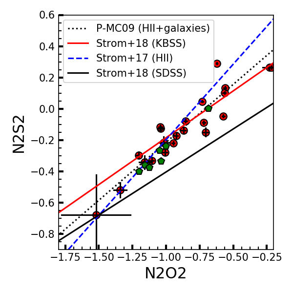
In Fig. 14 we first compare N2O2 with N2S2 with various relations from the literature. Strom et al. 2018 showed that KBSS galaxies at lie along a relation that is more similar to that found for local H ii regions (Pérez-Montero & Contini 2009; Strom et al. 2017) than typical star-forming galaxies from SDSS. LBAs occupy the region in between the relations for and H ii regions on one hand, and local SDSS galaxies on the other, with most LBAs being closer to the high redshift/local H ii lines. At a given N2O2, LBAs have higher N2S2 compared to typical SDSS galaxies. This behavior is very similar to that observed for local H ii regions and KBSS galaxies, and can be understood by the fact that LBAs and KBSS galaxies have star formation histories that are much simpler and more similar to H ii regions compared to typical SDSS star-forming galaxies (Sanders et al. 2016a; Kashino et al. 2017; Strom et al. 2018). Part of the [S ii] emission may arise from diffuse emission regions in between the H ii regions, lowering N2S2 in the case of more complex galaxies (Sanders et al. 2017).

In Fig. 15 we plot the strong line indicators for N/O (N2O2, N2S2, and N2) versus the direct N/O ratio. The majority of LBAs are concentrated in the region between and the solar value (horizontal dotted line). The smallest scatter is found for N2O2, which is not surprising because it is the most direct measure of N+/O+ among these three indicators. The LBAs lie along the relations found for KBSS galaxies and local H ii regions. The N2O2–N/O relation for H ii regions and galaxies from Pérez-Montero & Contini 2009 is known to be too steep, overestimating N/O for high N2O2 for both local H ii regions and high redshift galaxies (Strom et al. 2018). The relation between N/O and the strong line indicators found for the LBAs is more similar to the calibrations found for H ii regions and high redshift galaxies (Strom et al. 2017; Strom et al. 2018). Using only those objects in our sample for which the direct method N/O ratio is available, we fit the relation between N/O and N2O2, finding .


We will now determine whether the nitrogen-to-oxygen ratios of LBAs are in any way markedly different compared to either typical local or high redshift sources. In Fig. 16 we show the direct method nitrogen-to-oxygen ratio log(N/O)direct versus the stellar mass (left panel), and the direct method oxygen abundances. In both panels, we again give two sets of points, one calculated using T(O ii) as inferred from T(O iii) (filled circles) and the other using T(O ii) estimated from RO2 (open circles). In the left panel of Fig. 16, we are furthermore able to show a larger set of points by taking advantage of the best-fit relation between N/O and N2O2 determined for LBAs above (see left panel of Fig. 15). This allows us to include LBAs for which no direct-method N/O abundances could be measured. These estimates are indicate by the open squares. In the left-hand panel, it can be seen that the LBAs scatter around the typical N/O found for stacks of SDSS galaxies of a similar stellar mass (solid black line), which was also determined through the direct method by Andrews & Martini 2013. Kojima et al. 2017 find that their small sample of galaxies have N/O values comparable or smaller than this local relation, while Strom et al. 2017 find a somewhat lower N/O on average by dex for KBSS galaxies at compared to local SDSS galaxies with stellar masses in the range (red solid line in the left panel). However, in any case, these similar or somewhat lower values of N/O at fixed stellar mass are smaller than the typical downward offsets observed for LBAs in the O/H– relation (see Fig. 10). This implies that LBAs, and the samples from Kojima et al. 2017 and Strom et al. 2017, likely lie along a different N/O–O/H relation compared to typical local star-forming galaxies. We illustrate this in the right panel of Fig. 16, where we have indicated again the local sequence based on the SDSS stacks from Andrews & Martini 2013 as determined by Kojima et al. 2017 (solid black lines). The LBAs are, on average, offset toward higher N/O at fixed O/H.
The N/O excesses observed are of similar order of magnitude as those found for galaxies at by Kojima et al. 2017. The red dashed line in the right panel of Fig. 16 is the upper limit on the average N/O () for their sample, while the blue dashed line is the average N/O () they found for a sample of local galaxies selected to have similar (low) stellar masses and (high) star formation rates as their sample. Kojima et al. 2017 also noted that a stacked spectrum of the Steidel et al. 2016 sample of KBSS galaxies at falls close to their sample average (red dashed line), while green peas (which include several of the LBAs from our sample) span the range from no N/O excess to the average N/O for local, low mass, high star formation rate objects (blue dashed line). Our results for LBAs are in general agreement with those trends.
III.6 Origin of BPT offsets for Lyman Break Analogs
It has been known for some time that intensely star-forming galaxies at high redshift such as Lyman break galaxies, star-forming BzK galaxies, and distant red galaxies are often offset toward higher line ratios with respect to the mean SDSS star-forming population at low redshift in a standard BPT diagram (Teplitz et al. 2000; Shapley et al. 2005; Erb et al. 2006; Liu et al. 2008; Lehnert et al. 2009; Hayashi et al. 2009, e.g.). Such offsets were also found in some populations of low redshift galaxies, such as the “warm” infrared-luminous galaxies (Kewley et al. 2001) and Wolf–Rayet galaxies (Brinchmann et al. 2008a). These BPT offsets have been observed for LBAs as well (Hoopes et al. 2007; Overzier et al. 2008; Overzier et al. 2009, and Fig. 2 in this paper), further strengthening the conclusion that they are good local analogs of the high redshift star-forming population. Overzier et al. 2009 showed that the BPT displacement is in the sense of enhancements in one or both of [N ii]6584/H and [O iii]5007/H, and that the size of the perpendicular offset from the local star-forming ridge increases with both the luminosity of the brightest starburst clump and the electron density, indicating that higher star formation rate densities, interstellar densities and pressures, and ionization parameters may be related to the BPT offsets (Brinchmann et al. 2008b; Liu et al. 2008; Shirazi et al. 2014, e.g.).
In recent years, it has become feasible to address in more detail the physical origins of these BPT offsets, driven mainly by the wealth of near-infared spectroscopic data from new surveys of galaxies (Masters et al. 2014; Steidel et al. 2014; Shapley et al. 2015; Kashino et al. 2017, e.g.). Understanding how objects move through the BPT diagram, including the nature of the offsets, is extremely important, because the measurement of gas-phase abundances critically depends on the interpretation of ratios of the strong emission lines. This is particularly important at high redshift, where the temperature sensitive methods are often not available. There is therefore no guarantee that locally established calibrations are directly applicable. Various authors have found that high redshift objects display BPT offsets that are often larger than that can be explained by their increased ionization parameters and densities, and have shown that the BPT offset objects often have an increased N/O abundance and/or ionization parameter at high redshift compared to local galaxies for the same oxygen abundance (Masters et al. 2014; Shapley et al. 2015; Sanders et al. 2016a; Kojima et al. 2017, e.g.). Steidel et al. 2016, Strom et al. 2017 and Strom et al. 2018 showed that galaxies indeed have a higher N/O (at fixed excitation), and that N/O varies with O/H in a similar manner as observed for local H ii regions. Besides a higher N/O, they furthermore show the need for a harder ionizing spectrum at high redshift to fully explain the BPT offsets. These harder spectra could be a result of the differences in the star formation (and thus chemical enrichment) histories between typical local and high redshift galaxies.
In the previous sections, we have shown that at fixed O/H, LBAs have higher ionization parameters (Fig. 12) and higher N/O (Fig. 16, right panel) compared to typical local star-forming galaxies. Kojima et al. 2017 showed that galaxies at , as well as a small sample of local analogs consisting of LBAs, green peas and low mass/high SFR objects, display BPT offsets when either one of N/O or are increased, or both are increased. Positions along the BPT diagram are further modulated by the different O/H of the galaxies. The change in N/O (at fixed O/H) only affects the [N ii]6584/H ratio by an amount that directly corresponds to that change (a 0.3 dex increase in N/O gives a 0.3 dex change in [N ii]6584/H). The increase in is in the opposite direction as N/O, with some component along [O iii]5007/H that is roughly aligned along the star-forming ridge. At 12 + log(O/H)=8.10, a positive change of 0.3 dex in gives an increase in [O iii]5007/H of dex but a decrease in [N ii]6584/H of dex. Combined with the 0.3 dex increase in N/O, the total offset in the BPT diagram is toward higer values of both [O iii]5007/H and [N ii]6584/H, and in the direction observed for the galaxies studied.
In Fig. 17 we show again the location of LBAs in the BPT diagram, but with a color-coding determined by the offsets measured in N/O and relative to the local relations expectation given the O/H determined for each object through the direct method. The objects with the largest offsets in either parameter (or both) are expected to have the largest BPT offsets, which is indeed the case. The objects in our sample with the largest offsets lie around the average relation found by Steidel et al. 2014 for galaxies at . In the bottom right corner of the diagram, we find a number of massive and (likely) more metal-rich LBAs for which the [O iii]4363 flux could not be determined, and thus were not included in the analysis. We show the offsets measured perpendicularly from the local star-forming ridge as a function of the offsets in ionization parameter and N/O in Fig. 18. Objects with the largest perpendicular offsets (BPT⟂) indeed tend to have the largest offsets in (left panel) or log(N/O) (right panel) or both. From the analysis presented here, we thus conclude that the physical origin of the BPT offsets in LBAs are likely to be the same as those that explain the galaxies at and other types of local analogs thereof.

III.7 Possible origin of the excess N/O
As shown in Fig. 16, LBAs span a wide range of almost 1 dex in N/O values at a given O/H ratio. This wide scatter is similar to that observed for local H ii regions and the sample of KBSS galaxies at by Strom et al. 2018. These N/O values furthermore lie, on average, several tenths of dex above the typical N/O expected for local galaxies. This is similar to the trends observed for galaxies and other local analogs (Kojima et al. 2017; Strom et al. 2018, e.g.). What could be responsible for this N/O excess? The two most straightforward explanations are that N/O is increased either due to the presence of WR stars that enhance nitrogen on a time-scale that is shorter than the SNe enrichment (Hawley 2012, e.g.), or due to a decrease in O/H from the infall of a large quantity of low metallicity gas with the consequence that N/O appears spuriously high for the resulting O/H (Amorín et al. 2010; Masters et al. 2014, e.g.).
III.7.1 Evidence for WR stars
Galaxies with WR features often have enhanced N/O. Brinchmann et al. 2008a compared the average N/O between WR-enhanced galaxies and galaxies without WR features as a function of the equivalent width of H in order to control for difrerences that could arise due to secondary nitrogen production. In Fig. 19 we show the excess N/O as a function of the EW(H) for our sample. Brinchmann et al. 2008a found that the WR phase can be responsible for about dex excess N/O for objects with EW(H) below 100 Å, while above that the starbursts are typically younger than the phase where enrichment by WR winds occurs (thick solid line in Fig. 19). Several LBAs are known to have WR features. We have measured the strengths of the WR blue and red bumps in our sample, with two examples of objects with strong bumps shown in Fig. 20. In total we find 6 objects with clearly identifiable WR features (005527, 015028, 020356, 040208, BPT10 and HST03). These are marked in Fig. 19 with the large pentagons. Brown et al. 2014 also showed evidence for WR features in two additional LBAs (004054 and 092600). While some of the objects with the largest N/O excesses include objects with strong WR features in their spectra, the N/O excess is much larger than expected for WR galaxies. Furthermore, there appears to be no trend in Fig. 19 that relates the N/O excess with WR features or EW(H).


III.7.2 Evidence for infall of metal-poor gas
Besides nitrogen enhancement from WR stars, the rapid inflow of relatively metal-poor gas is an attractive alternative (or additional) scenario (Hwang et al. 2019, e.g.), especially given that most LBAs appear to be starbursts triggered by a recent interaction event (Overzier et al. 2008; Overzier et al. 2009). We showed that at a given stellar mass, LBAs have relatively low O/H with respect to the local MZR (Fig. 10), while they have normal N/O for their stellar mass (left panel of Fig. 16). They also have a lower O/H than expected based on their N/O (from the right panel of Fig. 16). This is exactly what would be expected for the accretion scenario. We can show this more clearly in Fig. 21, where we plot the offset in O/H with respect to the local MZR versus the offset in O/H with respect to the local average at a fixed N/O (from the right panel of Fig. 16). The good one-to-one correspondence between them implies that these offsets are one and the same, and related to the infall of a large quantity of metal-poor gas. In order to decrease O/H by 0.3 dex, the galaxy would need to accrete a quantity of metal poor gas equal to the mass of the ISM prior to the infall. On the secondary axes of Fig. 21 we have translated the offsets in O/H observed to the quantities of accreted metal-poor gas in units of the pre-infall gas mass. We have shown that the effect of the presence of WR stars on N/O is expected to be relatively limited, and furthermore is at odds with the normal N/O versus stellar mass relation (left panel of Fig. 16). We conclude that the recent gas accretion scenario can largely, or completely, explain the apparent N/O excesses observed.

IV Summary
In this paper, we analyzed VLT/XShooter spectra of a sample of LBAs to study the physical parameters of the interstellar medium in luminous UV-selected sources that share many properties with star-forming galaxies at high redshift. Our main findings are summarized as follows.
We estimated the electron densities and measured the electron temperatures T([OIII]) and T([OII]) for a subset of our sample, which allowed us to estimate direct oxygen abundances. The oxygen abundances of LBAs are in the range , confirming previous results based on strong-line methods that LBAs are, on average, offset from the local MZR (Fig. 10).
Comparing the direct method abundance estimates with those based on the O3N2 and N2 strong line ratios, we find general agreement within a scatter of 0.1–0.2 dex. This suggests that the strong line methods can be used for LBA-like galaxies at higher redshifts, as shown by other authors.
We determined the ionization parameter based on the index and the oxygen abundance, finding that LBAs have ionization parameters that are typically higher by up to 0.5 dex than typical star-forming galaxies of the same O/H (Fig. 12). We show that the SFR surface densities are correlated with the electron densities as expected for an ISM in which the pressure is regulated by the feedback from massive stars and supernovae. From the electron densities and the ionization parameter, we furthermore estimate the hydrogen-ionizing photon flux and show that it agrees remarkably well with the observed SFR surface density (Fig. 13).
We analyzed nitrogen abundance sensitive strong line ratios (N2O2, N2S2 and N2) and compare them with the N/O ratio determined through the temperature-sensitive method (Figs. 14 and 15). The LBAs tend to follow the same relations between these parameters found for both typical star-forming galaxies at as well as local H ii-regions (Strom et al. 2018, e.g.).
On avearge, LBAs lie on or close to the relation between N/O and stellar mass found for typical star-forming galaxies (left panel of Fig. 16), but above the typical N/O expected for galaxies at fixed O/H (right panel of Fig. 16).
We show that the offsets observed for LBAs in the BPT diagram are linked to the excesses in and/or N/O (Figs. 17 and 18). The relatively high ionization parameters, relatively low oxygen abundances, excess N/O and BPT offsets are of a similar order of magnitude as those observed by other authors for star-forming galaxies at as well as previously studied local analogs (Amorín et al. 2010; Brown et al. 2014; Masters et al. 2016; Sanders et al. 2016a; Steidel et al. 2014; Steidel et al. 2016; Strom et al. 2017; Kojima et al. 2017; Bian et al. 2018; Strom et al. 2018, e.g.).
Finally, we explore the origin of the N/O excess considering the two main scenarios proposed in the literature. We show that WR features observed in the spectra of some LBAs can explain at most a small fraction of the nitrogen enhancement (Figs. 19 and 20). The majority of the excess N/O, however, appears to be related to the recent inflow of large quantities of relatively metal-poor gas, which lowers O/H while leaving N/O unchanged. The relative decrease in O/H at fixed N/O is similar to the decrease in O/H at fixed stellar mass, and suggests that LBAs have experienced accretion of quantities of gas up to several times their original gas mass (Fig. 21). This is consistent with the conclusions of Amorín et al. 2010 based on strong line method abundances determinations for Green Pea galaxies and Lyman Break Analogs of Overzier et al. 2009.
The analysis performed in this paper highlights some of the difficulties of determining fundamental parameters such as ionization parameter, O/H, and N/O even in relatively nearby galaxies observed with 8-m telescopes. This illustrates some of the challenges we are faced with in determining these parameters and, more importantly, the physical processes that caused them, at much higher redshifts. This is important for upcoming observations with the James Webb Space Telescope which will give access to similar rest-frame optical emission line diagnostics for large samples of high redshift galaxies for the first time.
References
- Abazajian et al. (2009) Abazajian, K. N., Adelman-McCarthy, J. K., Agüeros, M. A., et al. 2009, ApJS, 182, 543
- Alexandroff et al. (2012) Alexandroff, R., Overzier, R. A., Paragi, Z., et al. 2012, MNRAS, 423, 1325
- Alexandroff et al. (2015) Alexandroff, R. M., Heckman, T. M., Borthakur, S., Overzier, R., & Leitherer, C. 2015, ApJ, 810, 104
- Amorín et al. (2010) Amorín, R. O., Pérez-Montero, E., & Vílchez, J. M. 2010, ApJ, 715, L128
- Amorín et al. (2012) Amorín, R., Pérez-Montero, E., Vílchez, J. M., & Papaderos, P. 2012, ApJ, 749, 185
- Andrews & Martini (2013) Andrews, B. H., & Martini, P. 2013, ApJ, 765, 140
- Asari et al. (2007) Asari N. V., et al., 2007, MNRAS, 381, 263
- Asplund et al. (2009) Asplund, M., Grevesse, N., Sauval, A. J., & Scott, P. 2009, ARA&A, 47, 481
- Baldwin et al. (1981) Baldwin, J. A., Phillips, M. M., & Terlevich, R. 1981, PASP, 93, 5
- Bian et al. (2016) Bian, F., Kewley, L. J., Dopita, M. A., & Juneau, S. 2016, ApJ, 822, 62
- Bian et al. (2017) Bian, F., Kewley, L. J., Dopita, M. A., & Blanc, G. A. 2017, ApJ, 834, 51
- Bian et al. (2018) Bian, F., Kewley, L. J., & Dopita, M. A. 2018, ApJ, 859, 175
- Blanton et al. (2001) Blanton, M. R., Dalcanton, J., Eisenstein, D., et al. 2001, AJ, 121, 2358
- Borthakur et al. (2014) Borthakur, S., Heckman, T. M., Leitherer, C., & Overzier, R. A. 2014, Science, 346, 216
- Bouwens et al. (2012) Bouwens, R. J., Illingworth, G. D., Oesch, P. A., et al. 2012, ApJ, 754, 83
- Bouwens et al. (2017) Bouwens, R. J., Illingworth, G. D., Oesch, P. A., et al. 2017, arXiv:1711.02090
- Bradley et al. (2012) Bradley, L. D., Bouwens, R. J., Zitrin, A., et al. 2012, ApJ, 747, 3
- Bradshaw et al. (2013) Bradshaw, E. J., Almaini, O., Hartley, W. G., et al. 2013, MNRAS, 433, 194
- Brinchmann et al. (2008a) Brinchmann, J., Kunth, D., & Durret, F. 2008a, A&A, 485, 657
- Brinchmann et al. (2008b) Brinchmann, J., Pettini, M., & Charlot, S. 2008b, MNRAS, 385, 769
- Brown et al. (2014) Brown, J. S., Croxall, K. V., & Pogge, R. W. 2014, ApJ, 792, 140
- Brown et al. (2016) Brown, J. S., Martini, P., & Andrews, B. H. 2016, MNRAS, 458, 1529
- Bruzual & Charlot (2003) Bruzual, G., & Charlot, S. 2003, MNRAS, 344, 1000
- Calzetti et al. (1994) Calzetti, D., Kinney, A. L., & Storchi-Bergmann, T. 1994, ApJ, 429, 582
- Calzetti (2001) Calzetti, D. 2001, PASP, 113, 1449
- Calzetti (2013) Calzetti, D. 2013, Secular Evolution of Galaxies, 419
- Cardamone et al. (2009) Cardamone, C., Schawinski, K., Sarzi, M., et al. 2009, MNRAS, 399, 1191
- Cardelli et al. (1989) Cardelli, J. A., Clayton, G. C., & Mathis, J. S. 1989, ApJ, 345, 245
- Chabrier (2003) Chabrier, G. 2003, PASP, 115, 763
- Chevalier & Clegg (1985) Chevalier, R. A., & Clegg, A. W. 1985, Nature, 317, 44
- Churchill & Vogt (2001) Churchill, C. W., & Vogt, S. S. 2001, AJ, 122, 679
- Cid Fernandes et al. (2005) Cid Fernandes R., Mateus A., Sodré L., Stasińska G., Gomes J. M., 2005, MNRAS, 358, 363
- Cid Fernandes et al. (2011) Cid Fernandes, R., Mateus, A., Sodré, L., Stasinska, G., & Gomes, J. M. 2011, Astrophysics Source Code Library, ascl:1108.006
- Conti (1991) Conti, P. S. 1991, ApJ, 377, 115
- Contursi et al. (2017) Contursi, A., Baker, A. J., Berta, S., et al. 2017, A&A, 606, A86
- Cowie, Barger & Songaila (2016) Cowie L. L., Barger A. J., Songaila A., 2016, ApJ, 817, 57
- Curti et al. (2017) Curti, M., Cresci, G., Mannucci, F., et al. 2017, MNRAS, 465, 1384
- Davé et al. (2011) Davé, R., Finlator, K., & Oppenheimer, B. D. 2011, MNRAS, 416, 1354
- Elmegreen et al. (2013) Elmegreen, B. G., Elmegreen, D. M., Sánchez Almeida, J., et al. 2013, ApJ, 774, 86
- Erb et al. (2006) Erb, D. K., Shapley, A. E., Pettini, M., et al. 2006, ApJ, 644, 813
- Fernandes et al. (2004) Fernandes, I. F., de Carvalho, R., Contini, T., & Gal, R. R. 2004, MNRAS, 355, 728
- Garland et al. (2015) Garland, C. A., Pisano, D. J., Mac Low, M.-M., et al. 2015, ApJ, 807, 134
- Garnett (1992) Garnett, D. R. 1992, AJ, 103, 1330
- Gburek et al. (2019) Gburek T., et al., 2019, ApJ, submitted (arXiv:1906.11849)
- Gonçalves et al. (2010) Gonçalves, T. S., Basu-Zych, A., Overzier, R., et al. 2010, ApJ, 724, 1373
- Gonçalves et al. (2014) Gonçalves, T. S., Basu-Zych, A., Overzier, R. A., Pérez, L., & Martin, D. C. 2014, MNRAS, 442, 1429
- Habouzit et al. (2017) Habouzit, M., Volonteri, M., & Dubois, Y. 2017, MNRAS, 468, 3935
- Hawley (2012) Hawley, S. A. 2012, PASP, 124, 21
- Hayashi et al. (2009) Hayashi, M., Motohara, K., Shimasaku, K., et al. 2009, ApJ, 691, 140
- Heckman et al. (1990) Heckman, T. M., Armus, L., & Miley, G. K. 1990, ApJS, 74, 833
- Heckman et al. (2005) Heckman, T. M., et al. 2005, ApJ, 619, L35
- Heckman et al. (2011) Heckman, T. M., Borthakur, S., Overzier, R., et al. 2011, ApJ, 730, 5
- Heckman et al. (2015) Heckman, T. M., Alexandroff, R. M., Borthakur, S., Overzier, R., & Leitherer, C. 2015, ApJ, 809, 147
- Heckman & Borthakur (2016) Heckman, T. M., & Borthakur, S. 2016, ApJ, 822, 9
- Hirschmann et al. (2017) Hirschmann M., Charlot S., Feltre A., Naab T., Choi E., Ostriker J. P., Somerville R. S., 2017, MNRAS, 472, 2468
- Hoopes et al. (2007) Hoopes, C., et al. 2007, Accepted for publication in the GALEX special issue of ApJS (astro-ph/0609415)
- Hwang et al. (2019) Hwang H.-C., et al., 2019, ApJ, 872, 144
- Izotov et al. (2006) Izotov, Y. I., Stasińska, G., Meynet, G., Guseva, N. G., & Thuan, T. X. 2006, A&A, 448, 955
- Izotov et al. (2007) Izotov, Y. I., Thuan, T. X., & Guseva, N. G. 2007, ApJ, 671, 1297
- Jaskot & Oey (2013) Jaskot, A. E., & Oey, M. S. 2013, ApJ, 766, 91
- Jia et al. (2011) Jia, J., Ptak, A., Heckman, T. M., et al. 2011, ApJ, 731, 55
- Kashino et al. (2017) Kashino, D., Silverman, J. D., Sanders, D., et al. 2017, ApJ, 835, 88
- Kauffmann et al. (2003) Kauffmann, G., Heckman, T. M., Tremonti, C., et al. 2003, MNRAS, 346, 1055
- Kausch et al. (2015) Kausch, W., Noll, S., Smette, A., et al. 2015, A&A, 576, A78
- Kewley et al. (2001) Kewley, L. J., Heisler, C. A., Dopita, M. A., & Lumsden, S. 2001, ApJS, 132, 37
- Kewley & Dopita (2002) Kewley, L. J., & Dopita, M. A. 2002, ApJS, 142, 35
- Kewley et al. (2006) Kewley, L. J., Groves, B., Kauffmann, G., & Heckman, T. 2006, MNRAS, 372, 961
- Kewley & Ellison (2008) Kewley, L. J., & Ellison, S. L. 2008, ApJ, 681, 1183
- Kewley et al. (2013) Kewley L. J., et al., 2013, ApJ, 774, 100
- Kobulnicky & Kewley (2004) Kobulnicky, H. A., & Kewley, L. J. 2004, ApJ, 617, 240
- Kobulnicky et al. (1999) Kobulnicky, H. A., Kennicutt, Jr., R. C., & Pizagno, J. L. 1999, ApJ, 514, 544
- Kojima et al. (2017) Kojima, T., Ouchi, M., Nakajima, K., et al. 2017, PASJ, 69, 44
- Köppen & Hensler (2005) Köppen, J., & Hensler, G. 2005, A&A, 434, 531
- Latif et al. (2018) Latif, M. A., Volonteri, M., & Wise, J. H. 2018, MNRAS, 476, 5016
- Lehnert et al. (2009) Lehnert, M. D., Nesvadba, N. P. H., Le Tiran, L., et al. 2009, ApJ, 699, 1660
- Leitherer et al. (1999) Leitherer, C., Schaerer, D., Goldader, J. D., et al. 1999, ApJS, 123, 3
- Liu et al. (2000) Liu X.-W., Storey P. J., Barlow M. J., Danziger I. J., Cohen M., Bryce M., 2000, MNRAS, 312, 585
- Liu et al. (2008) Liu, X., Shapley, A. E., Coil, A. L., Brinchmann, J., & Ma, C.-P. 2008, ApJ, 678, 758
- Lofthouse, Houghton & Kaviraj (2017) Lofthouse E. K., Houghton R. C. W., Kaviraj S., 2017, MNRAS, 471, 2311
- Maiolino et al. (2008) Maiolino, R., Nagao, T., Grazian, A., et al. 2008, A&A, 488, 463
- Martin et al. (2005) Martin, D. C., Fanson, J., Schiminovich, D., et al. 2005, ApJ, 619, L1
- Masters et al. (2014) Masters, D., McCarthy, P., Siana, B., et al. 2014, ApJ, 785, 153
- Masters et al. (2016) Masters, D., Faisst, A., & Capak, P. 2016, ApJ, 828, 18
- Mateus et al. (2006) Mateus A., Sodré L., Cid Fernandes R., Stasińska G., Schoenell W., Gomes J. M., 2006, MNRAS, 370, 721
- Meurer et al. (1999) Meurer, G. R., Heckman, T. M., & Calzetti, D. 1999, ApJ, 521, 64
- Modigliani et al. (2010) Modigliani, A., Goldoni, P., Royer, F., et al. 2010, Proc. SPIE, 7737, 773728
- Nakajima & Ouchi (2014) Nakajima, K., & Ouchi, M. 2014, MNRAS, 442, 900
- Osterbrock & Cohen (1982) Osterbrock, D. E., & Cohen, R. D. 1982, ApJ, 261, 64
- Östlin et al. (2014) Östlin, G., Hayes, M., Duval, F., et al. 2014, ApJ, 797, 11
- Overzier et al. (2008) Overzier, R. A., Heckman, T. M., Kauffmann, G., et al. 2008, ApJ, 677, 37
- Overzier et al. (2009) Overzier, R. A., Heckman, T. M., Tremonti, C., et al. 2009, ApJ, 706, 203
- Overzier et al. (2010) Overzier, R. A., Heckman, T. M., Schiminovich, D., et al. 2010, ApJ, 710, 979
- Overzier et al. (2011) Overzier, R. A., Heckman, T. M., Wang, J., et al. 2011, ApJ, 726, L7
- Patrício et al. (2018) Patrício, V., Christensen, L., Rhodin, H., Cañameras, R., & Lara-López, M. A. 2018, MNRAS, 481, 3520
- Pellegrini et al. (2012) Pellegrini, E. W., Oey, M. S., Winkler, P. F., et al. 2012, ApJ, 755, 40
- Pérez-Montero & Contini (2009) Pérez-Montero, E., & Contini, T. 2009, MNRAS, 398, 949
- Pérez-Montero (2017) Pérez-Montero, E. 2017, PASP, 129, 043001
- Pettini & Pagel (2004) Pettini, M., & Pagel, B. E. J. 2004, MNRAS, 348, L59
- Proxauf et al. (2014) Proxauf, B., Öttl, S., & Kimeswenger, S. 2014, A&A, 561, A10
- Rubin et al. (2010) Rubin, K. H. R., Weiner, B. J., Koo, D. C., et al. 2010, ApJ, 719, 1503
- Rubin et al. (2011) Rubin, K. H. R., Prochaska, J. X., Ménard, B., et al. 2011, ApJ, 728, 55
- Salim & Boquien (2018) Salim, S., & Boquien, M. 2018, arXiv:1812.05606
- Sanders et al. (2015) Sanders, R. L., Shapley, A. E., Kriek, M., et al. 2015, ApJ, 799, 138
- Sanders et al. (2016a) Sanders, R. L., Shapley, A. E., Kriek, M., et al. 2016a, ApJ, 816, 23
- Sanders et al. (2016b) Sanders, R. L., Shapley, A. E., Kriek, M., et al. 2016b, ApJ, 825, L23
- Sanders et al. (2017) Sanders, R. L., Shapley, A. E., Zhang, K., & Yan, R. 2017, ApJ, 850, 136
- Savage & Sembach (1996) Savage, B. D., & Sembach, K. R. 1996, ARA&A, 34, 279
- Schaerer & Vacca (1998) Schaerer, D., & Vacca, W. D. 1998, ApJ, 497, 618
- Schaerer et al. (2016) Schaerer D., Izotov Y. I., Verhamme A., Orlitová I., Thuan T. X., Worseck G., Guseva N. G., 2016, A&A, 591, L8
- Schlegel et al. (1998) Schlegel, D. J., Finkbeiner, D. P., & Davis, M. 1998, ApJ, 500, 525
- Schneider (2015) Schneider, P. 2015, Extragalactic Astronomy and Cosmology (England: Springer Heidelberg New York Dordrecht London), 626, bibliografia: p. 510–571
- Shapley et al. (2005) Shapley, A. E., Coil, A. L., Ma, C.-P., & Bundy, K. 2005, ApJ, 635, 1006
- Shapley et al. (2015) Shapley, A. E., Reddy, N. A., Kriek, M., et al. 2015, ApJ, 801, 88
- Shibuya et al. (2015) Shibuya, T., Ouchi, M., & Harikane, Y. 2015, ApJS, 219, 15
- Shim & Chary (2013) Shim, H., & Chary, R.-R. 2013, ApJ, 765, 26
- Shirazi et al. (2014) Shirazi, M., Brinchmann, J., & Rahmati, A. 2014, ApJ, 787, 120
- Shivaei et al. (2018) Shivaei I., et al., 2018, ApJ, 855, 42
- Smette et al. (2015) Smette, A., Sana, H., Noll, S., et al. 2015, A&A, 576, A77
- Spitzer (1968) Spitzer, L. 1968, Diffuse matter in space
- Stasińska & Leitherer (1996) Stasińska, G., & Leitherer, C. 1996, ApJS, 107, 661
- Steidel et al. (2014) Steidel, C. C., Rudie, G. C., Strom, A. L., et al. 2014, ApJ, 795, 165
- Steidel et al. (2016) Steidel, C. C., Strom, A. L., Pettini, M., et al. 2016, ApJ, 826, 159
- Strom et al. (2017) Strom, A. L., Steidel, C. C., Rudie, G. C., et al. 2017, ApJ, 836, 164
- Strom et al. (2018) Strom, A. L., Steidel, C. C., Rudie, G. C., Trainor, R. F., & Pettini, M. 2018, ApJ, 868, 117
- Teplitz et al. (2000) Teplitz, H. I., McLean, I. S., Becklin, E. E., et al. 2000, ApJ, 533, L65
- Wang et al. (2019) Wang B., Heckman T. M., Leitherer C., Alexandroff R., Borthakur S., Overzier R. A., 2019, ApJ, 885, 57
- Weiner et al. (2009) Weiner, B. J., Coil, A. L., Prochaska, J. X., et al. 2009, ApJ, 692, 187
- Woosley & Bloom (2006) Woosley S. E., & Bloom J. S. 2006, ARA&A, 44, 507
- Wu et al. (2019) Wu J. F., Baker A. J., Heckman T. M., Hicks E. K. S., Lutz D., Tacconi L. J., 2019, ApJ, in press (arXiv:1911.07854)
- Yates et al. (2019) Yates R. M., Schady P., Chen T.-W., Schweyer T., Wiseman P., 2019, A&A, accepted (arXiv:1901.02890)
| SDSS ID | IDa | Selectionb | COSc | R.A. | Dec. | Date | Seeinge | Modef | |
| (J2000) | (J2000) | FWHM (″) | |||||||
| J001009.97–004603.6 | 001009 | LBA | n | 00:10:09.97 | –00:46:03.66 | 0.243094 | 2010-11-07 | 1.7 | N |
| J001054.85+001451.3† | 001054 | LBA | n | 00:10:54.85 | 00:14:51.35 | 0.243141 | 2010-11-07 | 1.3 | O |
| J004054.32+153409.6 | 004054 | LBA | n | 00:40:54.33 | 15:34:09.66 | 0.283241 | 2010-11-08 | 1.4 | N |
| J005439.78+155446.9† | 005439 | LBA | n | 00:54:39.80 | 15:54:46.93 | 0.236400 | 2010-11-06 | 2.0 | N |
| J005527.45–002148.7 | 005527 | LBA | y | 00:55:27.46 | –00:21:48.71 | 0.167449 | 2010-11-07 | 1.1 | N |
| J015028.39+130858.4 | 015028 | LBA | y | 01:50:28.41 | 13:08:58.40 | 0.146712 | 2010-11-06 | 1.3 | N |
| J020356.91–080758.5 | 020356 | LBA | n | 02:03:56.91 | –08:07:58.51 | 0.188335 | 2010-11-07 | 1.1 | N |
| J021348.53+125951.4 | 021348 | LBA | y | 02:13:48.54 | 12:59:51.46 | 0.218962 | 2010-09-07 | 1.7 | N |
| J032845.99+011150.8 | 032845 | LBA | n | 03:28:45.99 | 01:11:50.85 | 0.142181 | 2010-10-05 | 1.8 | N |
| J035733.99–053719.6 | 035733 | LBA | n | 03:57:34.00 | –05:37:19.70 | 0.203746 | 2010-10-05 | 1.8 | N |
| J040208.86–050642.0 | 040208 | LBA | n | 04:02:08.87 | –05:06:42.06 | 0.139291 | 2010-10-05 | 1.9 | N |
| J143417.15+020742.5 | 143417 | LBA | n | 14:34:17.16 | 02:07:42.58 | 0.180325 | 2010-04-27 | 1.1 | O |
| J210358.74–072802.4 | 210358 | LBA | y | 21:03:58.75 | –07:28:02.45 | 0.136840 | 2010-08-10 | 1.6 | O |
| J214500.25+011157.5 | 214500 | LBA | n | 21:45:00.26 | 01:11:57.58 | 0.204321 | 2010-11-07 | 1.4 | N |
| J231812.99–004126.1 | 231812 | LBA | n | 23:18:13.00 | –00:41:26.10 | 0.251682 | 2010-11-06 | 1.7 | N |
| J232539.22+004507.2 | 232539 | LBA | n | 23:25:39.23 | 00:45:07.25 | 0.277000 | 2010-11-06 | 2.4 | N |
| J235347.69+005402.0 | 235347 | LBA | n | 23:53:47.69 | 00:54:02.08 | 0.223431 | 2010-10-08 | 1.4 | N |
| J124423.37+021540.4 | BPT03 | LBA2, BPT | n | 12:44:23.28 | 02:15:40.40 | 0.238964 | 2016-03-13 | 1.1 | N |
| J082247.66+224144.0 | BPT08 | LBA2, BPT | n | 08:22:47.75 | 22:41:44.10 | 0.216226 | 2016-03-12 | 2.1 | N |
| J101629.88+073404.9 | BPT09 | LBA2, BPT | n | 10:16:30.00 | 07:34:04.90 | 0.182710 | 2016-03-13 | 0.8 | N |
| J124509.05+104340.1 | BPT10 | LBA2, BPT | n | 12:45:09.12 | 10:43:40.00 | 0.165569 | 2016-03-12 | 1.4 | N |
| J084034.10+134451.3 | BPT11 | LBA2, BPT | n | 08:40:34.07 | 13:44:51.30 | 0.226961 | 2016-03-13 | 1.3 | N |
| J120735.77+082215.5 | BPT15 | LBA2, BPT | n | 12:07:35.76 | 08:22:15.50 | 0.204993 | 2016-03-13 | 1.3 | N |
| J102355.73+232338.6 | BPT20 | LBA2, BPT | n | 10:23:55.67 | 23:23:38.70 | 0.254211 | 2016-03-12 | 2.1 | N |
| J101009.90+205035.2 | BPT23 | LBA2, BPT | n | 10:10:09.83 | 20:50:35.50 | 0.209547 | 2016-03-12 | 2.1 | N |
| J120721.44+021657.7 | BPT26 | LBA2, BPT | n | 12:07:21.35 | 02:16:57.70 | 0.221747 | 2016-03-15 | 0.9 | N |
| J141612.87+122340.4 | HST03 | LBA2, COS | y | 14:16:12.96 | 12:23:40.50 | 0.123122 | 2016-03-12 | 2.1 | N |
| J104457.79+035313.1 | S012 | S2-Deficit | y | 10:44:57.84 | 03:53:13.10 | 0.012879 | 2016-03-13 | 1.3 | O |
| J095343.89–000524.7 | S041 | S2-Deficit | y | 09:53:43.91 | –00:05:24.60 | 0.083360 | 2016-03-15 | 1.4 | O |
| J122627.93+094456.6 | S091 | S2-Deficit | y | 12:26:27.84 | 09:44:56.70 | 0.090481 | 2016-03-15 | 0.9 | O |
| Originally part of the LBA sample, objects 001054 and 005439 were found to be AGN based on broad Mg II lines detected with XShooter. | |||||||||
| a. The number between parentheses is used to identify objects in certain figures. | |||||||||
| b. Sample selection (see text for details). | |||||||||
| c. Observed with the HST/COS spectrograph: ’y’ for yes, ’n’ for no. | |||||||||
| d. The systemic redshift was obtained from the SDSS spectra. | |||||||||
| e. Average seeing (FWHM) measured from the telluric standard star spectrum in the UVB arm. | |||||||||
| f. Observing mode: ’N’ for nodding, ’O’ for offset. | |||||||||
| ID | Emission line fluxesa,b,c | ||||||||||||
|---|---|---|---|---|---|---|---|---|---|---|---|---|---|
| [O ii]3727 | [O iii]4363 | H | [O iii]4959 | [O iii]5007 | [N ii]5755 | [N ii]6548 | H | [N ii]6584 | [S ii]6717 | [S ii]6731 | [O ii]7319 | [O ii]7330 | |
| BPT03 | 1762.1 8.6 | 75.81.4 | 867.9 6.7 | 1857.46.3 | 5412.414.8 | – | 38.61.0 | 2562.23.0 | 110.5 4.7 | 120.31.4 | 98.41.2 | 20.60.5 | 16.90.5 |
| BPT08 | 1879.540.5 | 60.91.6 | 899.4 9.6 | 1730.06.8 | 5229.313.7 | – | 85.51.6 | 2645.34.8 | 171.8 5.8 | 119.51.7 | 110.21.6 | 33.71.9 | 24.81.7 |
| BPT09 | 1655.311.4 | 42.51.7 | 728.810.8 | 1260.16.4 | 3816.313.8 | – | 51.71.1 | 2160.23.3 | 150.2 4.5 | 107.51.5 | 89.71.3 | 16.50.7 | 13.50.8 |
| BPT10 | 1534.9 6.3 | 24.60.7 | 864.8 5.5 | 1485.55.8 | 4429.910.6 | 2.70.5 | 63.11.0 | 2502.93.8 | 182.4 5.2 | 148.21.3 | 124.11.1 | 24.70.5 | 19.40.5 |
| BPT11 | 464.3 4.1 | 11.80.6 | 260.1 4.5 | 463.92.6 | 1392.3 5.3 | – | 20.30.6 | 758.41.8 | 62.6 2.3 | 47.90.9 | 38.10.8 | 7.20.3 | 5.70.5 |
| BPT15 | 557.8 4.8 | – | 213.8 4.1 | 171.02.7 | 507.9 4.6 | – | 49.31.1 | 626.82.0 | 153.3 2.6 | 59.91.1 | 52.81.0 | 6.10.6 | 5.10.8 |
| BPT20 | 341.2 7.3 | – | 206.2 4.9 | 124.93.0 | 369.9 4.7 | – | 104.61.6 | 606.02.2 | 280.9 2.5 | 51.61.5 | 47.71.5 | 7.31.2 | 4.80.9 |
| BPT23 | 605.670.6 | – | 237.4 8.9 | 53.94.8 | 159.7 7.4 | – | 122.32.5 | 703.63.5 | 357.8 3.4 | 107.42.4 | 87.12.2 | 1.21.8 | 13.21.6 |
| BPT26 | 380.829.3 | – | 304.717.7 | 43.38.0 | 158.614.8 | – | 204.24.0 | 934.64.9 | 569.2 5.7 | 98.83.0 | 102.33.1 | – | – |
| HST03 | 7803.546.1 | – | 2149.813.7 | 1718.938.5 | 5172.335.4 | 28.45.0 | 667.65.2 | 6465.28.0 | 1864.611.2 | 493.04.8 | 462.64.3 | 59.22.0 | 44.02.1 |
| S01 | 876.510.1 | 522.04.0 | 2907.3 9.9 | 3820.48.9 | 10006.9 18.0 | – | 9.71.2 | 8509.27.2 | – | 70.91.6 | 56.41.4 | 19.20.8 | 13.70.8 |
| S04 | – | – | 48.7 3.0 | 13.51.9 | 30.6 3.0 | – | 35.01.6 | 106.71.7 | 106.7 1.9 | – | – | – | – |
| S09 | – | – | 681.011.0 | 65.45.5 | 170.9 9.2 | – | 716.58.1 | 2041.07.2 | 1718.7 9.0 | 110.34.2 | 134.54.4 | 8.62.4 | 12.42.5 |
| 001009 | 122.3 2.7 | – | 47.6 2.3 | 33.61.4 | 90.7 2.2 | – | 7.70.5 | 138.51.1 | 24.0 1.0 | 19.21.1 | 14.80.9 | – | – |
| 004054 | 277.4 2.0 | 12.01.8 | 169.7 2.2 | 349.02.2 | 1044.6 4.7 | – | 5.80.5 | 493.51.3 | 19.2 1.7 | 23.70.7 | 18.60.6 | 3.90.8 | 3.31.0 |
| 005527 | 3234.830.0 | 35.91.8 | 1611.310.1 | 1991.98.7 | 5918.516.2 | 9.91.8 | 230.02.1 | 4751.85.4 | 599.6 7.2 | 284.82.3 | 253.42.1 | 56.60.9 | 43.80.9 |
| 015028 | 1344.910.3 | 10.01.2 | 605.916.1 | 449.84.4 | 1345.511.0 | – | 119.81.8 | 1786.23.4 | 366.9 4.1 | 155.71.6 | 133.61.5 | 11.40.5 | 9.50.8 |
| 020356 | 732.9 4.1 | 6.70.6 | 248.3 4.3 | 338.22.8 | 1002.4 6.3 | 2.00.3 | 19.70.6 | 722.91.6 | 57.3 2.0 | 70.21.1 | 53.01.0 | 6.50.3 | 5.50.4 |
| 021348 | – | – | 147.913.6 | – | 98.110.2 | – | 136.13.4 | 444.84.2 | 330.3 4.3 | 42.52.6 | 44.12.8 | – | – |
| 032845 | 605.7 3.3 | 3.60.5 | 281.2 2.6 | 206.21.9 | 645.0 4.0 | – | 35.70.9 | 815.41.6 | 115.6 2.1 | 80.11.0 | 61.60.8 | 6.50.3 | 5.40.4 |
| 035733 | 847.2 8.1 | – | 233.1 5.4 | 118.43.9 | 363.9 5.1 | – | 40.51.2 | 690.92.6 | 118.8 2.8 | 78.41.4 | 64.21.3 | 5.30.8 | 5.01.2 |
| 040208 | 373.9 2.8 | – | 104.0 2.1 | 89.31.7 | 259.1 3.4 | – | 11.60.6 | 303.01.2 | 36.6 1.4 | 41.31.1 | 28.30.8 | 3.00.4 | 1.90.6 |
| 143417 | 533.8 8.6 | – | 297.810.2 | 63.03.2 | 183.7 6.5 | – | 109.32.1 | 880.52.9 | 324.5 3.9 | 98.72.0 | 77.81.6 | – | – |
| 214500 | 554.3 4.1 | – | 213.3 3.4 | 88.22.3 | 266.4 3.3 | – | 48.30.9 | 623.21.9 | 148.2 2.3 | 93.81.2 | 71.31.0 | 4.80.6 | 3.61.1 |
| 231812 | 953.9 5.9 | – | 267.2 3.6 | 239.22.6 | 720.7 4.5 | – | 35.60.9 | 784.11.7 | 107.8 2.3 | 101.31.5 | 77.41.2 | 8.60.5 | 6.40.7 |
| 232539 | 237.6 2.7 | – | 101.4 2.9 | 135.01.7 | 413.3 3.5 | – | 6.80.7 | 295.81.6 | 22.9 1.9 | 22.80.9 | 15.00.7 | – | – |
| 235347 | 352.6 3.9 | 9.10.6 | 133.6 4.4 | 233.62.0 | 664.5 4.3 | – | 5.80.5 | 390.61.4 | 16.1 1.7 | 30.60.8 | 22.60.7 | 4.20.7 | 2.90.4 |
| a All line fluxes are given in units of erg s-1 cm-2. | |||||||||||||
| b Flux errors were determined by propagating the error spectra during the flux measurements, and do not include the uncertainties in the absolute flux calibration. | |||||||||||||
| c Line fluxes were corrected for Galactic and internal reddening, as well as stellar continuum absorption. | |||||||||||||
| SDSS ID | IDa | Selectionb | COSc | R.A. | Dec. | Referencee | |
| (J2000) | (J2000) | ||||||
| J004054.32+153409.6 | 004054 (L1) | LBA | n | 00:40:54.33 | +15:34:09.66 | 0.283241 | Amorín et al. 2012 |
| J113303.80+651341.3 | 113303 (L2) | LBA | n | 11:33:03.80 | +65:13:41.31 | 0.241 | Amorín et al. 2012 |
| J232539.22+004507.2 | 232539 (L3) | LBA | n | 23:25:39.23 | +00:45:07.25 | 0.277000 | Amorín et al. 2012 |
| J004054.32+153409.6 | 004054 (L4) | LBA | n | 00:40:54.33 | +15:34:09.66 | 0.283241 | Brown et al. 2014 |
| J005527.45–002148.7 | 005527 (L5) | LBA | y | 00:55:27.46 | –00:21:48.71 | 0.167449 | Brown et al. 2014 |
| J020356.91–080758.5 | 020356 (L6) | LBA | n | 02:03:56.91 | –08:07:58.51 | 0.188335 | Brown et al. 2014 |
| J092600.41+442636.1 | 092600 (L7) | LBA | y | 09:26:00.41 | +44:27:36.13 | 0.18072 | Brown et al. 2014 |
| a. The number between parentheses is used to identify objects in certain figures. | |||||||
| b. Selection of the target: ’LBA’ for objects from the sample of Heckman et al. 2005. | |||||||
| c. Observed with the HST/COS spectrograph: ’y’ for yes, ’n’ for no. | |||||||
| d. The systemic redshift was obtained from the SDSS spectra. | |||||||
| e. Reference from which the extinction-free, continuum absorption-corrected line fluxes were taken. | |||||||
| ID | log() | log() | log() | log([OIII]/H) | log([NII]/H) | log([SII]) | log([OII]) |
|---|---|---|---|---|---|---|---|
| (kpc-2) | (cm-3) | (cm-3) | |||||
| BPT03 | 9.59 | 10.7 | 9.66 | 0.79 | -1.37 | 2.26 | 2.39 |
| BPT08 | 9.58 | 10.5 | 9.15 | 0.77 | -1.19 | 2.55 | – |
| BPT09 | 9.46 | 10.5 | 9.28 | 0.72 | -1.16 | 2.31 | 2.34 |
| BPT10 | 9.58 | 10.7 | 9.42 | 0.71 | -1.14 | 2.32 | 2.5 |
| BPT11 | 9.29 | 10.4 | 9.20 | 0.73 | -1.08 | 2.16 | 2.23 |
| BPT15 | 10.4 | 10.5 | 9.81 | 0.38 | -0.61 | 2.45 | 2.72 |
| BPT20 | 10.1 | 10.6 | 9.66 | 0.25 | -0.33 | 2.55 | 2.9 |
| BPT23 | 10.7 | 10.6 | 9.74 | -0.17 | -0.30 | 2.23 | – |
| BPT26 | 10.8 | 10.6 | 9.84 | -0.28 | -0.22 | 2.76 | 2.8 |
| HST03 | 10.0 | 10.8 | 10.3 | 0.38 | -0.54 | 2.58 | 2.86 |
| S01 | 6.96 | 8.46 | 10.1 | 0.54 | -2.50 | 2.17 | 2.64 |
| S09 | 10.1 | 10.1 | 10.1 | -0.60 | -0.07 | 3.01 | – |
| 001009 | 10.5 | 10.5 | 9.47 | 0.28 | -0.76 | 2.05 | 1.58 |
| 004054 | 9.27 | 10.3 | 9.07 | 0.79 | -1.41 | 2.12 | 2.43 |
| 005527 | 9.69 | 10.6 | 10.1 | 0.57 | -0.90 | 2.47 | 1.47 |
| 015028 | 10.3 | 10.6 | 9.44 | 0.35 | -0.69 | 2.39 | 2.27 |
| 020356 | 9.41 | 10.6 | 9.30 | 0.61 | -1.10 | 1.95 | – |
| 021348 | 10.4 | 10.7 | 10.1 | -0.18 | -0.13 | 2.76 | – |
| 032845 | 9.82 | 10.4 | 9.08 | 0.36 | -0.85 | 2.03 | 2.19 |
| 035733 | 9.99 | 10.6 | 9.57 | 0.19 | -0.77 | 2.26 | 2.19 |
| 040208 | 9.50 | 10.4 | 9.51 | 0.40 | -0.92 | 1.99 | 1.99 |
| 143417 | 10.7 | 10.6 | 9.59 | -0.21 | -0.43 | 2.13 | 2.27 |
| 214500 | 9.98 | 10.5 | 9.93 | 0.10 | -0.62 | 1.98 | 2.26 |
| 231812 | 10.0 | 11.0 | 9.46 | 0.43 | -0.86 | 2.01 | 2.1 |
| 232539 | 9.27 | 10.6 | 9.72 | 0.61 | -1.11 | 2.24 | 2.24 |
| 235347 | 9.47 | 10.5 | 9.04 | 0.70 | -1.38 | 1.83 | 1.95 |
| ID | (O iii) | (O ii) | (N ii) | 12 + log(O/H) [N2] | 12 + log(O/H) [O3N2] | 12 + log(O/H) []a | log(N/O) []a | |
|---|---|---|---|---|---|---|---|---|
| ( K) | ( K) | ( K) | ||||||
| BPT03 | 1.20 0.01 | 0.94 0.02 | – | 8.120.01 | 8.040.01 | 8.270.01 | -1.470.02 | 7.940.01 |
| BPT08 | 1.14 0.01 | 1.09 0.05 | – | 8.220.01 | 8.110.01 | 8.390.02 | -1.400.02 | 7.950.01 |
| BPT09 | 1.13 0.01 | 0.83 0.03 | – | 8.240.01 | 8.130.01 | 8.330.02 | -1.340.02 | 7.850.01 |
| BPT10 | 0.94 0.01 | 1.14 0.02 | 0.99 0.09 | 8.250.01 | 8.140.01 | 8.540.01 | -1.310.03 | 8.060.01 |
| BPT11 | 1.05 0.02 | 1.16 0.05 | – | 8.280.01 | 8.150.01 | 8.370.03 | -1.170.03 | 7.970.02 |
| BPT15 | – | 0.84 0.06 | – | 8.550.01 | 8.410.01 | – | – | – |
| BPT20 | – | 1.21 0.16 | – | 8.710.01 | 8.540.01 | – | – | – |
| BPT23 | – | 1.06 0.16 | – | 8.730.01 | 8.690.01 | – | – | – |
| BPT26 | – | – | – | 8.780.01 | 8.750.02 | – | – | – |
| HST03 | – | 0.60 0.02 | 0.99 0.08 | 8.590.01 | 8.440.01 | – | – | – |
| S01 | 1.91 0.01 | 1.47 0.06 | – | 7.470.15 | 7.760.08 | 7.410.01 | -1.620.25 | 8.150.01 |
| S04 | – | – | – | 8.900.01 | 8.790.02 | – | – | – |
| S09 | – | 0.86 0.39 | – | 8.860.01 | 8.900.01 | – | – | – |
| 001009 | – | – | – | 8.470.01 | 8.400.01 | – | – | – |
| 004054 | 1.14 0.05 | 1.12 0.17 | – | 8.100.02 | 8.030.01 | 8.290.06 | -1.420.06 | 8.020.03 |
| 005527 | 0.96 0.01 | 1.14 0.02 | 1.03 0.09 | 8.390.01 | 8.260.01 | 8.470.02 | -1.140.01 | 7.840.01 |
| 015028 | 1.01 0.03 | 0.74 0.02 | – | 8.510.01 | 8.400.01 | 8.300.05 | -0.930.02 | 7.560.02 |
| 020356 | 0.98 0.03 | 0.86 0.03 | 1.51 0.15 | 8.270.01 | 8.180.01 | 8.430.05 | -1.410.03 | 7.710.02 |
| 021348 | – | – | – | 8.830.01 | 8.750.02 | – | – | – |
| 032845 | 0.94 0.03 | 0.94 0.03 | – | 8.420.01 | 8.340.01 | 8.300.06 | -1.060.02 | 7.580.02 |
| 035733 | – | 0.69 0.05 | – | 8.460.01 | 8.420.01 | – | – | – |
| 040208 | – | 0.76 0.06 | – | 8.380.01 | 8.310.01 | – | – | – |
| 143417 | – | – | – | 8.650.01 | 8.660.01 | – | – | – |
| 214500 | – | 0.81 0.07 | – | 8.540.01 | 8.500.01 | – | – | – |
| 231812 | – | 0.83 0.03 | – | 8.410.01 | 8.320.01 | – | – | – |
| 232539 | – | – | – | 8.270.02 | 8.180.01 | – | – | – |
| 235347 | 1.19 0.03 | 0.98 0.08 | – | 8.110.03 | 8.060.02 | 8.190.04 | -1.540.06 | 7.730.02 |
| a. Values were calculated by inferring (O ii) from (O iii) and the electron density. | ||||||||
| b. Ionization parameter as shown in Fig. 12. | ||||||||