The uncertainty of glass transition temperature in molecular dynamics simulations and numerical algorithm for its unique determination
Abstract
When the cooling rate is smaller than a certain material-dependent threshold, the glass transition temperature becomes to a certain degree the “material parameter” being nearly independent on the cooling rate. The common method to determine is to extrapolate viscosity of the liquid state at temperatures not far above the freezing conditions to lower temperatures where liquid freezes and viscosity is hardly measurable. It is generally accepted that the glass transition occurs when viscosity drops by orders of magnitude. The accuracy of depends on the extrapolation quality. We propose here an algorithm for a unique determining of . The idea is to unambiguously extrapolate to low temperatures without relying upon a specific model. It can be done using the numerical analytical continuation of -function from above where it is measurable, to . For numerical analytical continuation, we use the Pade approximant method.
I Introduction
Understanding processes of glass formation and jamming, and predicting the corresponding conditions, are among the main tasks in chemical physics. The question “why some liquids form a glass easily but others do not” has been thoroughly investigated Ediger et al. 1996; Cheng and Ma 2011; Ryltsev et al. 2013; Royall and Williams 2015. However, despite the decades of researches, there is still an unsolved problem related to uncertainty in the definition of glass transition temperature Stillinger and Debenedetti 2013.
Due to the fact that glass formation is dynamical non-equilibrium transition, the glass transition temperature depends strongly on the cooling procedure Fokin et al. 2005. In particular, there is a semiempirical relationship for cooling rate dependence of :
| (1) |
Here is the cooling rate, while and are material parameters. This expression can satisfactory fit experimental data in a variety of glassformers when is varied over 3 decades.
We consider here the “universal” limit when the cooling rate . Then the glass transition temperature becomes nearly independent on the cooling rate, , and so becomes to a certain degree the “material parameter”.
The common method for estimating the glass transition temperature is to determine the kinematic viscosity in the liquid state at temperatures not far above the freezing conditions. Usually this is temperature range of the order of 100 K. Then the temperature dependencies of is usually approximated by either the Arrhenius (strong glasses) or super-Arrhenius (fragile glasses) equations. The most widely accepted approximations for super-Arrhenius behaviour are the Vogel-Fulcher-Tamman formula (VF) Martinez-Garcia et al. 2014, where
| (2) |
and the power law from mode-coupling theory (MCT):
| (3) |
Here , , , , and are usually obtained by fitting these expressions with experimental data or results of computer simulations. For metallic glasses, the modification of VF-relation is often used Kawamura et al. 2001:
| (4) |
where , and are fitting parameters. There are many other fitting equations.
Having the fitting parameters, one can estimate the glass transition temperature by extrapolating the fitted to low temperatures above the singularity temperature where diverges.
It is generally accepted that the glass transition occurs when , where depending on a subjective choice. Uncertainty is built in this definition! The glass transition temperature depends on the choice of and the fitting equation. Generally, the dependence of from is quite weak while the choice of the extrapolating equation may sometimes give even uncertainty.
We propose here an algorithm for a unique determining of . The idea is to unambiguously extrapolate to a low-temperature region without relying upon a specific model. It can be done using the numerical analytical continuation of -function from above where it is measurable, to . For numerical analytical continuation, we use the Pade approximant method Baker Jr and Graves-Morris 1996.
Application of Pade approximation for numerical analytical continuation in physical problems has long history of success. This method, for example, has been successfully applied for extrapolations of the bulk-magnetization data to yield the Curie point; a good agreement is obtained if one assumes that the magnetization varies near the Curie temperature Craig et al. 1965; Chakraborty 1976. Near the Curi point of a dilute random substitutional ferromagnetic alloy, the magnetization varies as with between and . Such behavior suggests the possibility to describe the region of the Curie temperature by Pade-approximant calculations based upon Ising and Heisenberg models Craig et al. 1965; Baker Jr 2012. Pade approximation procedure has shown great success in cluster expansion methods Baker Jr 2012 and Dynamical Mean Field Theory (DMFT) Anisimov et al. 2009. It is one of the accepted methods for numerical analytical continuation (along with the maximum entropy method Kraberger et al. 2017) of Green functions from a discrete set of (imaginary) Matsubara frequencies to continuum of real frequencies Georges et al. 1996. A completely different application of Pade approximants refers to an accurate description of melting curves at high pressures Kechin 2001. Pade-based Kechin equations allowed to quantify all melting curves, rising, falling, and flattening, as well as curves with a maximum, on a universal basis.
Below we describe our method and give few illustrative examples.


II Methods
Pade approximants allow to interpolate and extrapolate a function specified by a table of points and, very importantly, to carry out an analytic continuation into the complex plane of the argument of the approximated function. The Pade approximant is defined through the rational function defined as the ratio of two polynomials. On the other hand, a rational function can be represented by a continued fraction, which approximates the function much more accurately compared to the series expansion. To construct the approximant, we use the “multipoint algorithm” Vidberg and Serene 1977. Suppose we know the values of a function at the points , where . Then the Pade approximant is constructed as follows:
| (5) |
where are determined from the condition , which holds if satisfy the relations
| (6) | |||
| (7) |
Expression (6) fulfills the role of the boundary condition for recursive relation (7). For example, taking , then we find from (6) and , from (7).
III Results
III.1 Repulsive shoulder system as the minimal model for glassformer
First, we consider the one-component system of particles interacting through repulsive core-softened potential Fomin et al. 2008 (Repulsive Shoulder System (RSS)) as the model glassformer. Earlier, we have shown that RSS demonstrates excellent glass-forming ability in certain density domain Ryltsev et al. 2013. The RSS potential has the following form:
| (8) |
Here . The unit of energy — , and are “hard”-core and “soft”-core scales. Taking these units, the dimensionless quantities are , , temperature , density , and time , where and are the molecular mass and system volume. Later we omit the tildes. We also choose , , and .
The RSS system at given parameters shows glass formation even in the universal limit with the cooling rate Ryltsev et al. 2013. We took data from Ref. Ryltsev et al. 2013 on the diffusion coefficient in the liquid phase not far above the glass transition threshold. The chosen density corresponds to the region with high glass-forming ability at the RSS phase diagram. We approximated using three different approaches: MCT, VF and Pade. After that low temperature extrapolation was performed to determine the glass transition temperature. The results are shown in Fig. 1. RSS is the superfragile glassformer Ediger et al. 1996; Ryltsev et al. 2013, so VF approximation is quite accurate. That explains why Pade approximant in Fig. 1 is close to VF. Fig. 1 may be considered as the stress test of the suggested Pade extrapolation method.
Data for extracted from Ref. Ryltsev et al. 2013 has low accuracy. In Fig. 1 this is even seen: the last data point corresponding to the lowest temperature is below the expected position. Such a low level of accuracy at first glance should prevent extrapolation by the analytical continuation method making it unstable. To solve this problem, we introduce averaging over two types of disorder into the calculation of the Pade approximant. We randomly remove 5% of the data before constructing the Pade approximant. Then we average the result over a large number of random samples. Also, we add small Gaussian noise to the data and average the result over it. These procedures allows to build extrapolation in the presence of the inaccurate data in Fig. 1.
The MD-data Ryltsev et al. 2013 used to draw Fig. 2 was more accurate than used to prepare Fig. 1. We even did not have to average over the Gaussian noise and random data samples during the Padé approximant construction.
Using Pade extrapolation method we were able to extract the critical temperature where goes to infinity. For fragile glassformers, this temperature is close to the so-called Kauzmann temperature Kauzmann 1948; Stillinger 1988; Ediger et al. 1996; Tanaka 2003; Kelton 2016, [The Kauzmann temperature is defined by intersection of the crystal entropy curve with that extrapolated for the supercooled liquid Stillinger 1988; Tanaka 2003.] Usually . In Figs. 1-2 we find as zero of Pade extrapolated . For RSS system we have got that calculated using VF and Pade nearly coincide. This is expected because RSS system is superfragile.
IV Experimental glassformers
IV.0.1 Glycerol
Now we take one of the most studied glass-forming systems, glycerol Kauzmann 1948; Bartos et al. 2001, to test our Pade-approximant method. According to Angell classification Ediger et al. 1996, glycerol is the fragile glassformer. So its viscosity varies with temperature not according to the Arrhenius activation law (as in strong glassformers) but more or less according to VF or MCT.
We took experimental data for the viscosity of glycerol Bartos et al. 2001 and used them to build the Pade approximant, see Fig. 3(a), where the viscosity of glycerol is plotted in log scale. Orange spheres show the experimental data and the blue curve corresponds to Pade approximant. In Fig. 3(b) viscosity is extrapolated into the complex plane of temperature to detect . It corresponds to the pole-singularity situated at the real axes of temperatures. We get K. This value is close to found in Bartos et al. 2001.
IV.0.2
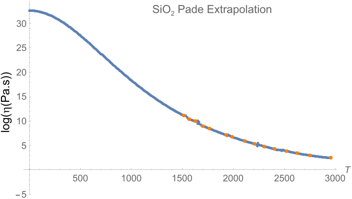
Now we consider which is an representative strong glassformer according to Angell classification. Its viscosity processed by Pade-method is shown in Fig. 4. Since the system demonstrates nearly Arrhenius temperature dependence of the viscosity, is not seen: Pade approximant is continuous at all temperatures.
IV.0.3
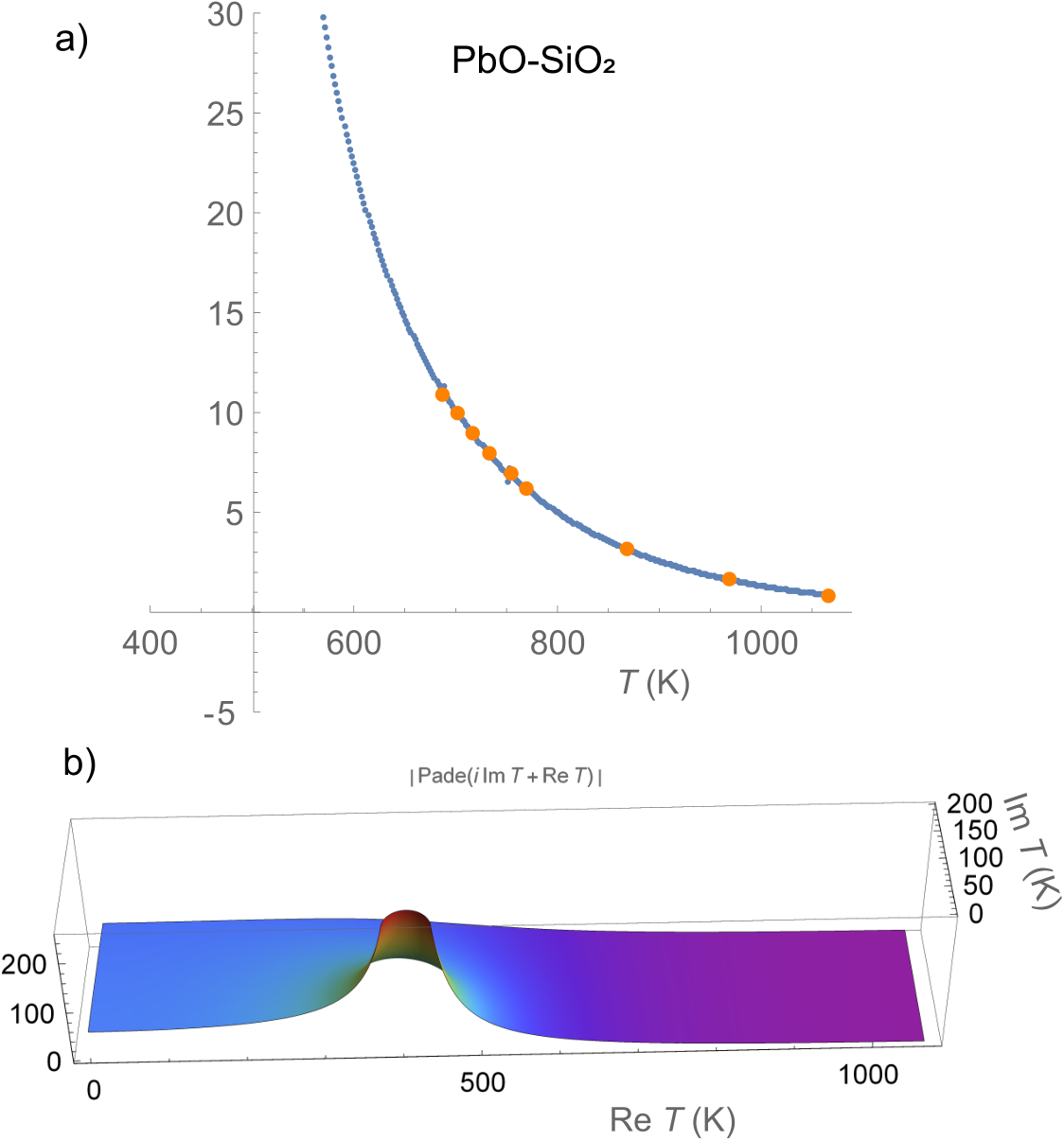
Now we take the fragile glassformer whose K has been estimated in Ref. Nascimento and Aparicio 2007 using VF approximation. We get K using Pade approximant, see Fig. 5. This result provides reasonable agreement.
Conclusions
We propose a method for unambiguous extrapolation of liquid kinetic coefficients to freezing temperatures. Our approach is based on numerical analytical approximation and error correction algorithms that allow overcoming instabilities related to inaccuracy of input data. Using the proposed method one can determine the freezing temperature and the critical temperature where liquid kinetic coefficients go to zero.
Acknowledgements.
We thank R. Khusnutdinov for stimulating discussions. This work was supported by the Russian Science Foundation (grant 18-12-00438). The numerical calculations are carried out using computing resources of the federal collective usage center ’Complex for Simulation and Data Processing for Mega-science Facilities’ at NRC ’Kurchatov Institute’ (http://ckp.nrcki.ru/), supercomputers at Joint Supercomputer Center of Russian Academy of Sciences (http://www.jscc.ru) and ’Uran’ supercomputer of IMM UB RAS (http://parallel.uran.ru).References
- Ediger et al. (1996) M. D. Ediger, C. A. Angell, and S. R. Nagel, The Journal of Physical Chemistry 100, 13200 (1996).
- Cheng and Ma (2011) Y. Cheng and E. Ma, Prog. Mater. Sci. 56, 379 (2011).
- Ryltsev et al. (2013) R. E. Ryltsev, N. M. Chtchelkatchev, and V. N. Ryzhov, Phys. Rev. Lett. 110, 025701 (2013).
- Royall and Williams (2015) C. P. Royall and S. R. Williams, Phys. Reports 560, 1 (2015).
- Stillinger and Debenedetti (2013) F. H. Stillinger and P. G. Debenedetti, Annual Review of Condensed Matter Physics 4, 263 (2013).
- Fokin et al. (2005) V. M. Fokin, M. L. Nascimento, and E. D. Zanotto, Journal of Non-Crystalline Solids 351, 789 (2005).
- Martinez-Garcia et al. (2014) J. C. Martinez-Garcia, S. J. Rzoska, A. Drzozd-Rzoska, J. Martinez-Garcia, and J. C. Mauro, Scientific reports 4, 5160 (2014).
- Kawamura et al. (2001) Y. Kawamura, T. Nakamura, H. Kato, H. Mano, and A. Inoue, Materials Science and Engineering: A 304-306, 674 (2001).
- Baker Jr and Graves-Morris (1996) G. Baker Jr and P. Graves-Morris, Padé approximants, Vol. 59 (Cambridge University Press, 1996).
- Craig et al. (1965) P. P. Craig, R. C. Perisho, R. Segnan, and W. A. Steyert, Phys. Rev. 138, A1460 (1965).
- Chakraborty (1976) K. G. Chakraborty, Journal of Physics C: Solid State Physics 9, 4411 (1976).
- Baker Jr (2012) G. A. Baker Jr, Quantitative theory of critical phenomena (Academic Press, 2012).
- Anisimov et al. (2009) V. I. Anisimov, D. M. Korotin, M. A. Korotin, A. V. Kozhevnikov, J. Kuneš, A. O. Shorikov, S. L. Skornyakov, and S. V. Streltsov, Journal of Physics: Condensed Matter 21, 075602 (2009).
- Kraberger et al. (2017) G. J. Kraberger, R. Triebl, M. Zingl, and M. Aichhorn, Phys. Rev. B 96, 155128 (2017).
- Georges et al. (1996) A. Georges, G. Kotliar, W. Krauth, and M. J. Rozenberg, Rev. Mod. Phys. 68, 13 (1996).
- Kechin (2001) V. V. Kechin, Phys. Rev. B 65, 052102 (2001).
- Vidberg and Serene (1977) H. J. Vidberg and J. W. Serene, Journal of Low Temperature Physics 29, 179 (1977).
- Fomin et al. (2008) Y. D. Fomin, N. V. Gribova, V. N. Ryzhov, S. M. Stishov, and D. Frenkel, J. Chem. Phys. 129, 064512 (2008).
- Kauzmann (1948) W. Kauzmann, Chemical Reviews 43, 219 (1948).
- Stillinger (1988) F. H. Stillinger, The Journal of Chemical Physics 88, 7818 (1988).
- Tanaka (2003) H. Tanaka, Phys. Rev. Lett. 90, 055701 (2003).
- Kelton (2016) K. F. Kelton, Journal of Physics: Condensed Matter 29, 023002 (2016).
- Bartos et al. (2001) J. Bartos, O. Sausa, J. Kristiak, T. Blochowicz, and E. Rössler, Journal of Physics: Condensed Matter 13, 11473 (2001).
- Nascimento and Aparicio (2007) M. L. F. Nascimento and C. Aparicio, Journal of Physics and Chemistry of Solids 68, 104 (2007).