Topology-Preserving Terrain Simplification
Abstract
We give necessary and sufficient criteria for elementary operations in a two-dimensional terrain to preserve the persistent homology induced by the height function. These operations are edge flips and removals of interior vertices, re-triangulating the link of the removed vertex. This problem is motivated by topological terrain simplification, which means removing as many critical vertices of a terrain as possible while maintaining geometric closeness to the original surface. Existing methods manage to reduce the maximal possible number of critical vertices, but increase thereby the number of regular vertices. Our method can be used to post-process a simplified terrain, drastically reducing its size and preserving its favorable properties.
Keywords:
Persistent Homology, Terrain, Terrain Simplification, Triangulation.1 Introduction
A terrain is a triangulated surface described by a scalar function defined on a finite set of points of and visualized as a height function of some topographic dataset, representing the mountains and valleys of a landscape. Terrains are a popular model to represent landscapes and play a fundamental role in areas such as cartography, computer graphics and computer vision.
In this work, we consider the problem of terrain simplification, also known as terrain approximation. We refer to [1, 2, 3] for extensive surveys on the topic and focus on the concepts important for our work. Generically, given a terrain over a domain, it asks for a “simpler” triangulation of the same domain which constitutes a “good” approximation of the original terrain . To make this setup concrete, we must specify the meaning of “good” and “simple”. For the former, a standard choice (which we also adopt throughout the paper) is to impose a maximal pointwise vertical distance between original and approximate terrain. Formally, for , we want that , where and are interpreted as scalar functions on a common domain. Another possible choice is to impose a quality criterion on the triangular mesh of (e.g., being a Delaunay mesh).
For defining “simplicity”, a default choice is ask for a terrain with fewer vertices, but natural formulations for this optimization problem are NP-hard (see the related work section below). Topological simplification is an alternative way to define simplicity, where the goal is to reduce the number of critical vertices (minima, maxima, saddles) of the terrain. Unlike in the previous case, the optimization problem is tractable: the algorithm by Bauer, Lange, and Wardetzky [4] (called BLW algorithm from now on) produces an -close terrain with the minimal number of critical points. As discussed in [4], such a “topologically clean” approximation is useful in many applications: for instance, in order to identify drainage basins, it is desirable to remove spurious minima that lead to a too fine fragmentation of the terrain. However, the drawback of the BLW algorithm is that realizing the topological simplification as a terrain requires a barycentric subdivision of the original triangulation, which increases the size of the terrain by a factor of and thus results in a severe performance penalty of subsequent steps.
The BLW algorithm makes use of the popular concept of persistence diagrams [5]. Such a diagram partitions the critical points into pairs such that and can both be removed from the terrain using a pointwise perturbation of persistence , which is the height difference of the two critical points. Bauer et al. show that it is possible to remove all critical pairs with with a single -perturbation. Since critical point pairs with cannot be cancelled in this way due to the stability of persistent homology [6], this proves the optimality.
Contributions
We investigate the following question: under what conditions does the persistence diagram of the terrain remain the same when (1) flipping an edge, or (2) removing a (regular) vertex and triangulating its link? For both cases, we propose sufficient and necessary conditions that can be checked locally (Section 3). While the edge flip condition can be checked in constant time, the vertex removal condition can be implemented with a algorithm with dynamic programming, where is the degree of the removed vertex. Both tests can be easily combined with testing for pointwise closeness, that is, whether an edge flip/a vertex removal yields a -close terrain with the same persistence.
Using the above test, we suggest a simple post-processing procedure for the output terrain of the BLW algorithm (Section 4): traverse the regular vertices and greedily remove vertices without changing the persistence diagram, always maintaining an -close terrain, until no further vertex can be removed. Note that maintaining the persistence diagram implies that the number of critical points remains the same. Hence, the result of our post-processing still achieves the minimal number of critical points, but is smaller in size.
We experimentally evaluate our method (Section 5). For instance, on a terrain with K vertices, the BLW algorithm yields a topologically clean terrain with about K vertices. Our post-processing yields a topologically equivalent terrain that only consists of K vertices. Hence, our method addresses the major drawback of the BLW algorithm of returning a too large terrain.
The above example can be computed in about 2 minutes on a workstation. Achieving this running time requires several algorithmic ideas. One of them is a heuristic improvement of the BLW algorithm to avoid computing the entire barycentric subdivision. Our implementation is based on Cgal’s arrangement package [7] and uses exact number types for numerical computations. The code is available in a public repository11 1 https://bitbucket.org/mkerber/terrain_simplification..
Motivation and further related work
Bajaj and Schikore [8] outline a reduction method that is similar to ours: they propose to remove vertices from the terrain and re-triangulate, such that the resulting terrain is -close and all vertices retain their “criticality type” (i.e., being regular, a minimum, saddle or maximum). We show that preserving the persistence diagram is equivalent to this condition. While they outline a method for checking whether a re-triangulation meets their conditions, they do not describe how to find such a triangulation efficiently, and they do not report on experimental results.
Our approach is motivated by the area of hierarchical models of terrains, where one aims for a multi-resolution representation of a terrain that should reflect the essential properties of the terrain at various levels of detail. To create such representation, it is useful to act on geometric and topological properties of the terrain separately. Several algorithms for modifying the topology while maintaining the triangulation of the terrain have been proposed [9, 10, 11, 12, 13, 14]; our approach can be seen as acting in the other direction, maintaining topology and simplifying the triangulation. Formerly proposed methods described in [15, 16] aim for a similar goal, but they focus on the restricted case of edge contractions and on how such operators affect discrete Morse gradient vector fields.
The BLW algorithm is an improvement over previous simplification algorithms by Attali et al. [17] and Edelsbrunner et al. [18] which are not guaranteed to remove all critical points of persistence . As with the BLW algorithm, these algorithms require a barycentric subdivision, so our method can be combined with these algorithms as well.
Our work investigates the practical aspects of terrain reduction and does not discuss the optimality of our (greedy) removal strategy. Without topological constraint, the problem is already difficult; precisely, the problem of finding the smallest terrain that is -close to an input terrain is NP-hard [19] but approximation algorithms [20] and many heuristic approaches with weak or no guarantees on the size of the approximation (e.g., [21]) exist.
2 Background notions
Triangulated terrains
A terrain is a triangulation of a compact polygonal region in , possibly with internal vertices, endowed with an injective scalar function called height function defined on its set of vertices ; the injectivity of is just assumed for simplicity in the write-up but our implementation does not require it. Using barycentric coordinates, we can piecewise-linearly extend the height function to the entire domain of . Based on that, a terrain is always associated with a triangulated surface in obtained as the graph of such an extended height function (see Figure 1 for an example). Whenever this will not cause any ambiguity, we will make no distinction between considering a terrain as a triangulation in endowed with a height function or as the corresponding surface. Given two terrains and defined on the same polygonal region , we define .


A vertex is called interior if it is not on the boundary of the triangulated domain. For an interior vertex , the link of consists of all the vertices adjacent to as well as all the edges of such that is a triangle in . The lower link of a vertex of is the collection of vertices and edges in such that and , respectively. Analogously, the upper link is the collection of vertices and edges in satisfying the above equations in which is replaced with . Let us call an interior vertex regular if both and are non-empty and connected. Otherwise, will be called critical. As an example, in Figure 1(a), vertex 10 is regular and vertices 17 and 24 are critical.
Persistent homology of a terrain
Given a value , we write for all points in the domain whose height is at most . Then , and we call the piecewise-linear (PL) filtration of the terrain.
 |
 | |
| (a) | (b) |
Persistent homology [22, 23, 5] enables us to study the topological changes occurring during a filtration. In our concrete case, persistence tracks the evolution of connected components and holes in the terrain while the height function is increasing (see Figure 2). It can be proven that, modulo a suitable handling of the boundary vertices, there is a one-to-one correspondence between the critical points of and the homological changes in its filtration [4]. The information gathered by persistent homology is summarized in a combinatorial structure called the persistence diagram (or equivalently, the barcode).
It will be convenient to work with a different filtration in our setting. For each point of a terrain , we define as the lowest-dimensional cell (vertex, edge, triangle) that contains . Assuming that is spanned by boundary vertices with , we set , and , and call the simplex-wise filtration of the terrain. Note that is not continuous in , so the sets change discontinuously at vertex values. Nevertheless, we still have that , so the persistent homology of the simplex-wise filtration is well-defined. See Figure 2 for an illustration.
It is well-known (e.g., [4]) that the PL filtration and the simplex-wise filtration yield identical persistence diagrams. This follows from the fact that, for every , and, moreover, there is a deformation retraction [24] from to . This implies that the inclusion map induces an isomorphism of homology groups. We will use the same condition for the equality of persistence diagrams several times in this text.
3 Persistence-preserving operations on terrains
Persistence-preserving edge flip
Given a terrain and an interior edge , let and be the two triangles incident to such that the quadrilateral is convex. In that case, we call an edge flip the operation of removing and its two adjacent triangles from the terrain and replacing them with the edge and the triangles and , resulting in a new terrain (with coincides with outside the quadrilateral ).
For two vertices of , we define the real interval
We call the edge topologically flippable if . See Figure 3 for an example.
Proposition 1
Let be a terrain with an edge as above, and let denote the terrain after flipping the edge . The edge is topologically flippable if and only if the terrains and have the same persistence diagrams.
Proof 1
We can, without loss of generality, assume that the height values of in are and that the height of is equal to . Then, there only exist three combinatorial configurations for the quadrilateral , which are depicted in the leftmost column of rows , , and of Figure 3. The edge is the vertical edge in each picture. Rows , , and show the corresponding flipped situation.
Using the fact that the persistence diagram of a terrain is determined by its simplex-wise filtration, it is enough to compare the simplex-wise filtrations at the critical values , , , and . The right-hand columns of Figure 3 show the sublevel sets of the filtrations at these values inside the quadrilateral (outside the quadrilateral, both terrains coincide).
Comparing row and , we observe that the filtration of is included in the filtration of for each critical value (even though that inclusion does not respect the simplicial structure in the rightmost column). We observe that the inclusion from into is a deformation retract at value , and trivially also at any other position because the filtrations are equal everywhere else. It follows that the two filtrations have the same persistence diagram. The same argument can be applied to row and , switching the roles of and . This proves the “if” part of the statement.
Comparing row and , we observe for critical value , the sublevel sets of and differ by exactly one edge. By the Euler-Poincaré formula [5], the homology groups of the two sublevel sets differ, which implies that the persistence diagrams are not equal. This proves the “only if” part.
The proof also reveals that if an edge is not topologically flippable, the two persistence diagrams differ by at most the distance of and in bottleneck distance (see [5] for the definition). This might be of interest in variants of simplification where a small change of persistence is acceptable.
Persistence-preserving vertex removal
Given a terrain and an interior vertex of with exactly incident edges, the vertex removal of is the operator which removes from together with its incident edges and triangles, and triangulates the link of using a set of diagonals, resulting in the terrain . See Figure 4 for an illustration.
Again, we are interested in circumstances under which the persistence diagrams of and coincide. A necessary condition is that is regular, as one can readily check. If the link of is a triangle, it is also sufficient.
Proposition 2
Let be a regular vertex of with three incident edges. Then, the vertex removal of yields a terrain with the same persistence diagram as .
Proof 2
Note that because the link of is a triangle, no diagonals are necessary for the re-triangulation. Denoting the three adjacent vertices of as , , and , we can assume that have heights and since is regular, its height is either or . Figure 5 depicts both possible situations. In both cases, it can be observed, as in the proof of Proposition 1, that the persistence diagrams are the same.
For arbitrary vertex removals, we have generally several choices for triangulating the link. To characterize which triangulations are persistence-preserving, we use the following concept.
Definition 1
Let be a vertex of with two adjacent vertices , such that . We call the edge persistence-aware if one of the following conditions holds:
- 1.
;
- 2.
and there is a path on the link of from to with maximal height ;
- 3.
and there is a path on the link of from to with minimal height .
An example is depicted in Figure 6.
Theorem 3
Let be a regular interior vertex of of degree . Let denote the terrain obtained by removing and re-triangulating its link with diagonals. If all diagonals are persistence-aware, and have the same persistence diagram.
The proof idea is illustrated in Figure 7. We point out that the converse is also true, and the condition is also equivalent to the statement that all vertices in the link maintain their criticality status. See A for the proofs of these statements.
Proof 3
Without loss of generality, we assume that . We prove the statement by induction on . Note that because is not on the boundary. The case follows from Proposition 2. For , we write for the triangulation of the link of using the persistence-aware diagonals. An ear in a triangulation of a polygon is a triangle where both and are polygon edges, and only is a diagonal. It is a well-known fact [25] that every triangulation of a polygon with vertices has at least two ears.
We call an ear irregular if and have the same sign and has the opposite sign, and regular otherwise. Note the the presence of an irregular ear implies that either the lower or the upper link of consists of the vertex only (because is regular). Consequently, can have at most one irregular ear, and hence, must have at least one regular ear.
Now, let denote a regular ear of . The idea is to flip the edge of to obtain the edge , which results in losing one vertex in its link, and to use induction. Let us first make the simplifying assumption that is outside of the triangle , hence forms a convex quadrilateral. We argue that , which implies that flipping does not change the persistence diagram by Proposition 1: if the signs of and differ, this is clear because . If the signs of and are the same, the sign of is the same, because the ear is regular. We assume that all signs are positive; the negative case is analogous. Because the edge is persistence-aware, there is a path on the link where all height values are at least . The path from to that does not pass through passes through the lower link of and hence contains at least one vertex with negative height. So, the only path that can have the property asserted by persistence-awareness is . This implies .
Let denote the terrain obtained from by flipping . As we just argued, and have the same persistence diagram. In , has degree . Moreover, the remaining diagonals (apart from ) triangulate the link of in , and it can be readily checked that they are all persistence-aware, because they were persistence-aware in . Hence, by induction, we can re-triangulate the link without changing the persistence diagram, and the claim follows.
It remains to deal with the case that is inside the (regular) ear. In this situation, the quadrilateral is not convex, and the edge flip introducing yields to crossings. A first idea might be to just relocate inside the polygon (the position of inside the polygon has no effect on the persistence diagram). It is possible, however, that the relocated might not see all boundary vertices anymore (see Figure 8 (left)).
Instead, we can resolve this issue by not insisting that the edges of a terrain are straight lines. We omit a formal description of the argument for the sake of simplicity and outline the proof idea. A topological triangulation is a planar embedding of a graph where all bounded faces are bounded by three edges. In a topological triangulation, an edge flip can always be realized, possibly by bending edge, as displayed in Figure 8 (right). We can also define the simplex-wise filtration of topological triangulations because the filtration only depends on the elevation of the vertices and the combinatorial structure of the triangulation; in particular, the filtration, and the resulting persistence diagram are independent of the actual planar embedding. Also, the definition of links and persistence-aware diagonals, and all results from this section extend to the topological case. In that way, we obtain a topological triangulation with diagonals and the same persistence diagram as the initial one. But, since we obtain the diagonals by cutting off ears, a simple inductive argument shows that these diagonals do not cross when embedded as straight-line segments. This allows us to “straighten” the final triangulation and finishes the proof.
4 Algorithm
Reduction method
We give an algorithm for the following problem: given , a base terrain and a terrain with , compute a terrain with fewer vertices than , such that and and have the same persistence diagram. Note that is allowed, in which case one obtains a -close approximation of with the same topological information. In our application, however, will be the input terrain, and will be the result of the BLW algorithm, arising from a subdivision of .
The algorithm idea is to start with and incrementally removing vertices from , maintaining the condition on the -distance and the persistence diagram as specified above. For that, we proceed as follows: we maintain a set of candidate vertices (initially set to all vertices of ). While this set is non-empty, we choose a candidate vertex uniformly at random, remove it from the candidate set and check whether it can be removed and its link can be triangulated maintaining the condition. If yes, we remove from and add the edges of the link triangulation. We re-insert the vertices of the link to the candidate set, if not already contained, and start over. This finishes the description of the algorithm.
Testing edges and triangles
The major primitive of the above algorithm is to find a triangulation of the link of a vertex that maintains the algorithm’s condition (or to output that there is none). We call a vertex removable if such a triangulation exists. To characterize removable vertices, we need the following definitions. Let denote the height function of and the height function of . For two vertices , of (not necessarily connected via an edge), we call the line segment -aware if for any point on the line segment , we have that . In other words, if was an edge of the terrain , the -distance of and is at most along the edge. Similarly, for three vertices , , of , we call the triangle -aware if for any point of the triangle, we have that .
Lemma 4
A vertex is removable if there is a triangulation of its link such that all diagonals of the triangulation are persistence-aware and -aware, and all triangles of the triangulation are -aware.
Proof 4
Let denote the terrain before the removal of , and the terrain when removing and inserting the triangulation. Since both diagonals and triangles of the link triangulation are -aware, is -close to in the area enclosed by the link, and hence on the entire domain, because it coincides with everywhere else. The persistence diagrams of and are equal by Theorem 3 because all diagonals are persistence-aware.
Note that checking whether a diagonal is persistence-aware can be done by simply traversing the link once, yielding a primitive with the size of the link. The -awareness tests are based on the following results, which reduces the locations where the height difference is maximized to a finite set.
Lemma 5
The -distance of to along an edge is maximized at , at , at a crossing of with an edge of , or at an intersection of with a vertex of .
The -distance of to in a triangle is maximized at a boundary edge or vertex of , or at a vertex of inside the triangle.

Hence, for checking -awareness of edges, it suffices to compute the zone of in (i.e., the set of vertices, edges, and faces of traversed by ) and check the height difference at most one point per element in the zone. The running time is dominated by computing the zone of .
For checking the -awareness of triangles, it suffices to compute the -awareness of its boundary edges and to additionally check the height difference for all vertices of within . We obtain these vertices by a triangular range query in , and the running time is dominated by the complexity of this range query - see B.
Finding a triangulation
The above primitives to check persistence- and -awareness allow us to investigate a fixed triangulation. However, the naive application of Lemma 4 by just trying all triangulations is prohibitive because of the exponential number of possible triangulations of the link. We describe a simple dynamic programming approach.
Let denote the link polygon and let its vertices be denoted by in counterclockwise order. Let , and define as the subpolygon spanned by vertices . The idea is that any triangulation of has one triangle incident to the edge , where . To determine whether has a valid triangulation with triangle , it suffices to check whether the edges and are persistence- and -aware, whether the triangle is -aware, and whether the subpolygons and admit a valid triangulation (if or , the corresponding test can be skipped). We simply iterate through all until a valid triangulation is found or all values of have been tested. Applying this procedure to yields an algorithm to check whether a vertex is removable (and computes a valid triangulation in the positive case).
The above procedure operates on subpolygons of the form with and we can thus store all intermediate answers using quadratic space. We also store the persistence- and the -awareness of every edge when computed, using quadratic space as well. Hence, the procedure requires a total of such awareness tests on edges, and -awareness tests on triangles in the worst case.22 2 There is no reason to store the results on triangles since every triangle is queried only once.
Mesh improvement
With similar ideas, we can also describe a greedy procedure to improve the quality of the triangulation of a terrain, without sacrificing its geometric and topological properties. The input are two terrains and , and the output is a terrain , with the same relations as in the reduction phase, with the difference that has the same number of vertices as .
The idea is reminiscent of the well-known edge-flipping algorithm for turning an arbitrary triangulation into a Delaunay triangulation just by greedily flipping edges to increase the minimal angle locally [25]: we flip the edge to the edge if is persistence- and -aware, the two incident triangles to are -aware, and the flip improves the minimal angle. We maintain a set of candidate edges (initially all edges of ) and flip a candidate if the described criteria are met. We repeat until no candidate remains.
The BLW algorithm
We use the topological simplification algorithm from [4] as described in detail in the PhD thesis of Bauer [26]. We also use the symmetrizing approach [4, Section 6.2] to reduce the -perturbation per cell.
The output of the BLW algorithm is a simplex-wise function on the input triangulation , that is, we obtain a filtration value for each vertex, edge, and face of the triangulation. In order to convert this into a terrain, we pass to the barycentric subdivision of , and assign to each vertex of the filtration value of as its height. It is known that the terrain obtained in this way has the same persistence diagram as the initial function [4, Thm 7]. However, in order to satisfy the -constraint, we might have to place the vertex very close to one of the vertices (see Figure 10), which yields a poor quality mesh and numerical instability (if an imprecise number type is used). In general, such a placement might even be impossible (see also [17, Section 4.3]), but our solution works under the assumption that is chosen generically, meaning that is not equal to the height difference of any two input vertices. We refer to B for details of our placement method.
Avoiding subdivisions
Since our final goal is to remove as many vertices as possible, it is beneficial to avoid subdividing edges and triangles if possible. We devise a simple heuristic for that: if the BLW algorithm assigns to an edge the same value as to one of its boundary vertices, we do not subdivide this edge. Moreover, if the BLW algorithm assigns to a triangle the same value as to one of its corner vertices and none of the three boundary edges is subdivided, the triangle is not subdivided. This procedure can create a situation that a triangle is subdivided, but only some (or none) of its boundary edges are. In that case, the vertex of the face is connected with the corner vertices and the vertices of subdivided boundary edges (see Figure 11). The correctness of the method comes from the observation that for each step the filtrations of the fully subdivided and partially subdivided terrain coincide.
The whole pipeline
We summarize the entire algorithmic pipeline that we use. The input is a terrain and some , such that is not equal to the difference of two heights. The output is another terrain that is -close to in -distance and has the smallest number of critical points possible.
- 1.
Apply the BLW algorithm on to get a terrain with the specified properties.
- 2.
Apply the reduction method on to get a smaller terrain with the same properties.
- 3.
Apply the mesh improvement algorithm on and return the output.
5 Implementation and experiments
Implementation details
We implemented the algorithm described in Section 4 using C++. The program is available in a public repository33 3 https://bitbucket.org/mkerber/terrain_simplification. and it consists of about 3000 lines of code.
Our implementation makes extensive use of the functionality provided by the Cgal library (version 4.14)44 4 CGAL, Computational Geometry Algorithms Library, https://www.cgal.org.. For representing terrains, we decided to use Cgal’s 2D arrangement package [7] instead of a triangulation data structure, because it provides more flexibility in the removal and re-triangulating procedure. Moreover, it contains the basic functionality to traverse the zone of a line segment in an arrangement, needed for checking the -constraint for edges. For triangular range queries, we wrote our own algorithm – see B.
We point out that our geometric primitives cannot assume generic position of the vertices of the terrain. Even if this was assumed for the input , subdividing an edge yields a triple of collinear points by design. Moreover, as mentioned above, the subdivision approach might place vertices very close to existing ones. To avoid instabilities due to these effects, our implementation uses exact number types both for coordinates of points and height values (provided by Cgal’s Exact_predicates_exact_construction_kernel [27]).
Examples
We demonstrate the various steps of the proposed implementation with some examples. We have considered datasets coming from two different sources: [28] provides an altitude value for each point of a regular grid representing Styria, a state of Austria; [29] contains a collection of terrain models representing the area around some lakes in Italy (see Figure 12).
 |
 |
| (a) | (b) |
For both the classes of terrains, we have studied datasets of various sizes by considering all the provided points or a subsample of them. We focus here on a representation of Styria of K vertices (mentioned in the introduction), performing on it the proposed reduction strategy by choosing as -constraint meters. Despite the drastic reduction in size to K vertices, the input and the output terrains look pretty similar (see Figure 13).
 |
 |
| (a) | (b) |
The first step of the proposed simplification strategy consists in performing the BLW algorithm. The topological simplification performed by BLW is based on a barycentric subdivision of the input terrain. As discussed in the previous section, this step can be improved by avoiding a certain number of subdivisions. Figure 14 depicts cutouts of the input terrain, of the fully subdivided, and of the partially subdivided terrain. We observed that triangles involved in subdivisions in Figure 14(c) tend to form paths in the mesh surface rather than being randomly spread.
 |
 |
 |
| (a) | (b) | (c) |
The last step of our algorithm improves the quality of the reduced terrain by flipping edges to increase the minimal angle. In general, only a rather small fraction of edges is flipped in this step (around 10% in the above example). Nevertheless, we can visually see local improvements, as depicted in Figure 15.
 |
 |
| (a) | (b) |
Performance
We ran our implementation on a workstation with 6 CPU cores with 3.5 GHz per core and 64 GB of RAM, running Ubuntu 16.04.5. Our tests do not exploit the multi-core architecture and run on a single core.
In Table 1, we present the output size and the running time of our procedure for subsamples of the Styria dataset. The sampled points were chosen uniformly at random. For each size, we ran the algorithm times and display the average running time and the maximal deviation from the average. For all runs, we picked meters.55 5 An analogous table reporting the performances obtained for the lake datasets is presented in C.
| I | S | C | O | T |
|---|---|---|---|---|
| 10K | 17K | 407 | 4100.6 () | 8.90 () |
| 20K | 33K | 543 | 6114.2 () | 19.96 () |
| 40K | 64K | 547 | 8654.2 () | 38.96 () |
| 80K | 124K | 597 | 11223.2 () | 81.19 () |
| 160K | 239K | 611 | 13160.2 () | 168.54 () |
| 320K | 455K | 637 | 15019.0 () | 342.40 () |
First of all, we see that our method creates terrains of much smaller size compared to the output of the BLW algorithm, and even much smaller than the input terrain. Our sparser subdivision strategy generally decreases the number of points by a factor of about compared to the full barycentric subdivision whose size is around six times as large as the input size. This decrease leads to a a substantial saving of running time. We also see that the output size and the number of critical points in the output terrain increase slowly compared to the input size. This is not surprising because a finer sampling of the landscape is unlikely to create persistent topological features or drastic changes in the -distance. Moreover, we observe that the deviation from the average is small in all cases, so the algorithm is rather stable regarding its randomized removal strategy.
The running time of the algorithm splits into about 9-10% for creating the initial arrangement data structure out of the input, 9-10% for computing the BLW simplification, 78-80% for the reduction and around 2% for the final edge flips (for all problem sizes). Hence, the reduction step is the bottleneck of the computation, but its performance is less than an order of magnitude away from the other steps.
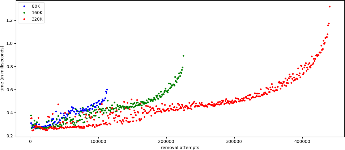
We also observe that the running time is slightly super-linear. To further investigate this, we look at the average running time for an attempted vertex removal (successful or not) at various stages of the algorithm. Figure 16 shows the average timings, averaged over around 1000 attempts. We observe three things: first, the time per attempts is almost the same at the beginning of the algorithm, independent of the input size. This shows that the reduction step is indeed a local operation and only depends mildly (i.e., logarithmically) on the size of the terrain. Second, we see that time per attempt gradually increases during the algorithm, which is explained by the increased cost of computing a zone in the arrangement when the edges get longer. Finally, we observe that the running time increases significantly towards the end of the algorithm. This is due to the fact that the algorithm has more failed attempts towards the end, and failed attempts tend to be more costly than successful ones because more triangles need to be checked.
Variants for vertex removal
We experimented with two variants of our method: recall that in our original version, when re-triangulating the link of a vertex , we stop when a valid triangulation is found. Instead, we can also keep checking and return the valid triangulation with minimal -distance to the previous terrain. The idea is that a smaller distance will be beneficial in subsequent steps to remove more vertices. As we see in Table 2, this strategy indeed yields a modest decrease in the final number of vertices, in exchange for a small slow-down of the method.
| Strategy 1 | Strategy 2 | Strategy 3 | ||||
|---|---|---|---|---|---|---|
| I | O | T | O | T | O | T |
| 10K | 4094.6 | 9.00 | 4087.8 | 11.15 | 4063 | 47.73 |
| 20K | 6120.0 | 19.15 | 6095.0 | 25.00 | 6081 | 128.21 |
| 40K | 8648.2 | 39.41 | 8619.4 | 53.49 | 8623 | 365.91 |
| 80K | 11206.4 | 81.23 | 11128.6 | 115.62 | 11142 | 1233.32 |
| 160K | 13165.4 | 164.83 | 13065.6 | 246.52 | 13090 | 4943.32 |
| 320K | 15031.0 | 328.15 | 14911.6 | 516.66 | 14915 | 21167.50 |
We have also implemented and tested a more elaborate approach where among all candidates that can be removed, we select the one whose removal causes the smallest -perturbation to . Similar to the previous variant, it appears beneficial to remove vertices first that cause small geometric distortion. This strategy requires, however, to initially check all vertices of to determine the best candidate. Also, after every vertex removal, all neighbors have to be re-checked. Table 2 shows that this strategy does not lead to a noticeable decrease in the output size, but is substantially increases the runtime. We remark that already initialization phase consumes about 50% of the running time of the randomized strategy. Hence, we do not see a justification for this approach.

The effect of
The output size of our algorithm clearly depends on the chosen . In Figure 17, we display the size in dependence on the values chosen. For very small values of , the BLW algorithm does not change the height of any vertex, edge, or triangle, meaning that our subdivision strategy keeps the input terrain. For very large values of , the BLW algorithm removes all critical vertices, and our reduction method can remove all interior vertices, only leaving the boundary vertices. For -values in between, we observe that the size is monotonously decreasing. For instance, the terrain size gets halved at around meters.
6 Conclusions and discussion
We presented a method to reduce the total size of a topologically simplified terrain, overcoming a major drawback of previous simplification methods without giving up on its guarantees. We showed experimentally that the performance is satisfying using the Cgal library. We see room for further improvements, for instance, by using better heuristics to avoid subdivisions in the BLW algorithm, by using an inexact, yet numerically robust number type, and by parallelizing our greedy removal procedure.
It is quite simple to see that our removal strategy does not always yield the smallest possible terrain. While in practice, many vertices can be removed, the complexity for finding an optimal reduction (for a fixed ) is open. It would also be interesting to investigate how far our output is from an optimal solution, both for the worst case and in expectation.
Since Cgal’s arrangement package is able to represent arrangements on surfaces (such as spheres and tori), it will be simple to extend our implementation to run on piecewise-linear functions on triangulated surfaces as well. We pose the question whether there are problems for which a simplification method as described will be useful.
Acknowledgments
Partially supported by the Austrian Science Fund (FWF) grant number P 29984-N35, by the Italian MIUR Award “Dipartimento di Eccellenza 2018-2022” - CUP: E11G18000350001, and by the SmartData@PoliTO center for Big Data and Machine Learning technologies. The authors thank Ulrich Bauer and Efi Fogel for helpful discussions.
References
- [1] P. S. Heckbert, M. Garland, Survey of polygonal surface simplification algorithms, Tech. rep., Carnegie-Mellon University of Pittsburgh (1997).
- [2] J. Talton, A short survey of mesh simplification algorithms, Tech. rep., University of Illinois at Urbana-Champaign (2004).
- [3] P. Cignoni, C. Montani, R. Scopigno, A comparison of mesh simplification algorithms, Computers & Graphics 22 (1) (1998) 37–54. doi:10.1016/S0097-8493(97)00082-4.
- [4] U. Bauer, C. Lange, M. Wardetzky, Optimal topological simplification of discrete functions on surfaces, Discrete & Computational Geometry 47 (2) (2012) 347–377. doi:10.1007/s00454-011-9350-z.
- [5] H. Edelsbrunner, J. Harer, Computational topology: an introduction, American Mathematical Soc., 2010.
- [6] D. Cohen-Steiner, H. Edelsbrunner, J. Harer, Stability of persistence diagrams, Discrete & Computational Geometry 37 (2007) 103–120. doi:10.1007/s00454-006-1276-5.
- [7] R. Wein, E. Berberich, E. Fogel, D. Halperin, M. Hemmer, O. Salzman, B. Zukerman, 2D arrangements, in: CGAL User and Reference Manual, 5.0 Edition, CGAL Editorial Board, 2019.
- [8] C. L. Bajaj, D. R. Schikore, Topology preserving data simplification with error bounds, Computers & Graphics 22 (1) (1998) 3 – 12. doi:10.1016/S0097-8493(97)00079-4.
- [9] P.-T. Bremer, H. Edelsbrunner, B. Hamann, V. Pascucci, A topological hierarchy for functions on triangulated surfaces, IEEE Transactions on Visualization and Computer Graphics 10 (4) (2004) 385–396. doi:10.1109/TVCG.2004.3.
- [10] T. Weinkauf, D. Günther, Separatrix persistence: extraction of salient edges on surfaces using topological methods, Comput. Graph. Forum 28 (5) (2009) 1519–1528. doi:10.1111/j.1467-8659.2009.01528.x.
- [11] A. Gyulassy, N. Kotava, M. Kim, C. Hansen, H. Hagen, V. Pascucci, Direct feature visualization using Morse-Smale complexes, IEEE Trans. on Visualization and Computer Graphics 18 (9) (2012) 1549–1562. doi:10.1109/TVCG.2011.272.
- [12] D. Günther, J. Reininghaus, H. Wagner, I. Hotz, Efficient computation of 3D Morse-Smale complexes and persistent homology using discrete Morse theory, The Visual Computer 28 (10) (2012) 959–969. doi:10.1007/s00371-012-0726-8.
- [13] L. Čomić, L. De Floriani, F. Iuricich, Simplification operators on a dimension-independent graph-based representation of Morse complexes, in: C. L. L. Hendriks, G. Borgefors, R. Strand (Eds.), ISMM, Vol. 7883 of Lecture Notes in Computer Science, Springer, 2013, pp. 13–24. doi:10.1007/978-3-642-38294-9_2.
- [14] R. Fellegara, F. luricich, L. De Floriani, K. Weiss, Efficient computation and simplification of discrete Morse decompositions on triangulated terrains, in: Proceedings of the 22Nd ACM SIGSPATIAL International Conference on Advances in Geographic Information Systems, SIGSPATIAL ’14, ACM, New York, NY, USA, 2014, pp. 223–232. doi:10.1145/2666310.2666412.
- [15] F. Iuricich, L. De Floriani, Hierarchical Forman triangulation: a multiscale model for scalar field analysis, Computers & Graphics 66 (2017) 113–123. doi:10.1016/j.cag.2017.05.015.
- [16] T. K. Dey, R. Slechta, Edge contraction in persistence-generated discrete Morse vector fields, Computers & Graphics 74 (2018) 33 – 43. doi:10.1016/j.cag.2018.05.002.
- [17] D. Attali, M. Glisse, S. Hornus, F. Lazarus, D. Morozov, Persistence-sensitive simplification of functions on surfaces in linear time, Presented at TOPOINVIS 9 (2009) 23–24.
- [18] H. Edelsbrunner, D. Morozov, V. Pascucci, Persistence-sensitive simplification functions on 2-manifolds, in: Proceedings of the Twenty-second Annual Symposium on Computational Geometry, SCG ’06, ACM, New York, NY, USA, 2006, pp. 127–134. doi:10.1145/1137856.1137878.
- [19] P. K. Agarwal, S. Suri, Surface approximation and geometric partitions, SIAM Journal on Computing 27 (4) (1998) 1016–1035. doi:10.1137/S0097539794269801.
- [20] P. K. Agarwal, P. K. Desikan, An efficient algorithm for terrain simplification, in: Proceedings of the Eighth Annual ACM-SIAM Symposium on Discrete Algorithms, SODA ’97, Society for Industrial and Applied Mathematics, Philadelphia, PA, USA, 1997, pp. 139–147.
- [21] M. Eck, T. DeRose, T. Duchamp, H. Hoppe, M. Lounsbery, W. Stuetzle, Multiresolution analysis of arbitrary meshes., in: Siggraph, Vol. 95, 1995, pp. 173–182. doi:10.1145/218380.218440.
- [22] H. Edelsbrunner, D. Letscher, A. Zomorodian, Topological persistence and simplification, Discrete & Computational Geometry 28 (4) (2002) 511–533. doi:10.1007/s00454-002-2885-2.
- [23] S. Oudot, Persistence theory: from quiver representation to data analysis, Vol. 209 of Mathematical Surveys and Monographs, American Mathematical Society, 2015.
- [24] A. Hatcher, Algebraic topology, Cambridge University Press, 2002. doi:10.1017/S0013091503214620.
- [25] M. De Berg, M. Van Kreveld, M. Overmars, O. C. Schwarzkopf, Computational geometry, algorithms and applications, in: Computational geometry, Springer, 2000, pp. 1–17.
- [26] U. Bauer, Persistence in discrete Morse theory. PhD thesis (2011).
- [27] H. Brönnimann, A. Fabri, G.-J. Giezeman, S. Hert, M. Hoffmann, L. Kettner, S. Pion, S. Schirra, 2D and 3D linear geometry kernel, in: CGAL User and Reference Manual, 5.0 Edition, CGAL Editorial Board, 2019.
- [28]
Land Steiermark,
Styria
10m digital terrain model (2020).
URL https://www.data.gv.at/katalog/dataset/land-stmk_digitalesgelndemodell10m - [29]
D. S. WorkBench,
Aim@Shape
repository (2006).
URL http://visionair.ge.imati.cnr.it/ontologies/shapes/ - [30] M. Bäsken, 2D range and neighbor search, in: CGAL User and Reference Manual, 5.0 Edition, CGAL Editorial Board, 2019.
Appendix A Proof details for persistence-aware triangulations
We first show the converse of Theorem 3.
Theorem 6
Let be a regular interior vertex of of degree . Let denote the terrain obtained by removing and re-triangulating its link with diagonals. If and have the same persistence diagram, all diagonals are persistence-aware.
Proof 5
By reductio ad absurdum, assume that an edge is not persistence-aware. That means, and are either both in the lower link or the upper link of . Let us consider the case first that both are in the upper link. On the upper link path from to , there must exist a vertex whose height value is smaller than the height of and of . We claim that and have different homology in the sublevel set at scale or at . See Figure 18 for an illustration. In general, is indeed not connected to any link vertex at scale in , just because the edge separates it from all vertices in the link with smaller height value. On the other hand, is connected to in . Hence, at scale , the simplex-wise filtration of adds exactly and the edge , whereas the simplex-wise filtration of only adds (and no edge within the link). Both filtrations might add additional edges and triangles outside of the link, but these are the same for both terrains. It follows that the filtration of adds exactly one more cell at scale than the simplex-wise filtration of . It follows (by considering the Euler characteristic and the Euler-Poincaré formula) that the homology groups differ either before or at . This proves the statement for the upper link case.
For the lower link case, let be the vertex on the lower link path between and with maximal height . Similar to the previous case, we claim that the simplex-wise filtrations of and add numbers of cells at height of different parity, implying that the homology groups have to differ before or after . See Figure 19 for an illustration.
Again, it suffices to count the number of cells added within the link, since both terrains are identical outside the link. For , at height , the vertex and its two incident edges on the link are added, resulting in cells in total. In , the non-persistence-aware edge ensures that is not adjacent to a link vertex with larger height. It follows that, at height , the filtration adds all edges incident to . Let denote its degree. Also triangles between consecutive edges incident to get added, because is the maximal vertex of the triangle. This yields triangles in total. It follows that vertex, edges, and triangles are added, resulting in a total of addition, which is an even number.
A vertex of is a minimum if all its neighbors have larger height, or equivalently, if its upper link is a cycle. It is a maximum if its upper link is empty. It is regular if its upper link is simply-connected. It is a -saddle with if its upper link consists of connected components. Every vertex is either a minimum, maximum, regular points, or -saddle, and we call its type the criticality type of the vertex. Note that we consider a -saddle and a -saddle to be of different criticality type. The following statement shows the connection of our method with the approach by Bajaj and Schikore [8].
Theorem 7
Let be a regular interior vertex of of degree . Let denote the terrain obtained by removing and re-triangulating its link with diagonals. All vertices of (except ) have the same criticality type in if and only if all diagonals are persistence-aware.
Proof 6
By inspection of Figures 3 and 5 that flipping a topologically flippable edge and removing a regular vertex with a triangular link does not change the criticality type of any vertex in the link. In the proof of Theorem 3, we showed that we can reduce the link of a regular vertex to a triangle with flips of topologically flippable edges. Hence, in this sequence, no vertex changes the criticality type, proving one direction of the theorem.
For the other direction, assume that is not persistence-aware. If and are in the upper link, let be the vertex on the upper link path between and with minimal height. Let and denote the two neighbors of along the link of . In , the link of has a connected component in the lower link that consists only of because the two neighbors of on the link of are and , which are both higher than by the choice of . In , is removed from the link of , and possibly replaced by a sequence of other vertices in the link of . However, the presence of the non-persistence-aware edge ensures that all vertices that become incident in have a larger height than . It follows that the lower link of loses a connected component from to , which means that either also the upper link loses a component or the upper link becomes a cycle. In both cases, the vertex changes its criticality type. The argument for a non-persistence-aware lower link edge is symmetric.
Appendix B Algorithmic details
Proof of Lemma 5
If the first statement was wrong, the only remaining possibilities are that a maximum occurs at a point in a face of , or at a point where overlaps with an edge of . In both cases, both and along around are constant or linear functions. There difference is either a linear function (which has no local maximum) or constant, in which case the same height difference is also attained at a vertex of either or .
If the second statement was wrong, the only possibilities are that the maximum occurs at a point on an edge of or inside a face of it. In the former case, is a constant or linear function along the edge, and the same is true for . This means that the difference is either a linear function (contradicting the assumption of a maximum at ), or constant, in which case the maximum is also achieved at a vertex of or the boundary of the triangle. The case that is in a triangle of work in the same way, choosing an arbitrary line through .
Placement of subdivision vertices
We describe first the placement of a vertex of that corresponds to an edge of . Let , , and the function values returned by the BLW algorithm for the vertices and the edge. Assume, without loss of generality, that . By the filtration property, also must hold. With Lemma 5, it suffices to place the vertex of at point on the interior of the line segment such that , where denotes the height of in the terrain . We try to find such a point that is as central as possible between and .
Note the following problem (also addressed in [17]): if (that is, is pushed upwards by the full ) and (that is, the height along the edge is not constant), we have that for every point in the interior of , and a valid placement of the vertex for is impossible. We thus assume, for simplicity, that is chosen so that no persistence pair of has persistence exactly . In that case, there exists such that the BLW algorithm applied on still removes all persistence points of persistence , and every cell changes its function value by strictly less than .
Now, we are looking for such that
A simple calculation yields the condition
By assumption, , hence the right hand side is strictly smaller than . We choose
and place the subdivision vertex for edge at .
For a triangle , assume that is the vertex with maximal height. Let be the midpoint of . We then compute a point in the interior of the line segment (which lies in the interior of the triangle), such that the distance of and is at most , with the same formula as above.
Triangular range queries
Given three points , , , we want to report all vertices of that are on or inside the triangle . We remark that Cgal offers an algorithm for this problem in the 2D range and neighbor search package [30] which is based on Delaunay triangulations. More precisely, this algorithm computes all points in the circumcircle of and checks each encountered point for being inside the triangle or not. This solution is unsatisfying for very flat triangles, where the circumcenter becomes so large that many false positives are found. In that case, the running time of the algorithm depends on the number of vertices of , in theory and in practice.
Instead, we use the following approach: initially, mark all vertices of as unvisited. Let denote a queue that is initially empty. For each boundary edge, we compute its zone in the arrangement . The zone contains all edges of that cross the triangle boundary. For every such edge, we check its endpoints whether they are unvisited and in the triangle. If yes, we mark the vertex as visited, put in into and report the vertex. For all vertices of in the zone, we proceed in exactly the same way.
Then, we pop elements from . For each vertex, we traverse its neighbors in . When a neighbor is unvisited an in the triangle, we mark it as visited, add it to and report it. We terminate when is empty.
For the complexity of this approach, note that computing the zone of a line segment has an (expected) complexity of , where is the size of the zone, where the logarithmic factor comes from point location for the first endpoint of the line segment in . Denoting by the sum of the zones of the three triangle edges, the complexity is , with the number of vertices reported.
Appendix C Additional experimental results
Table 3 presents the output size and the running time of our simplification procedure for uniform subsamples of the lake datasets. We always picked meters and we display the average execution time of 5 runs and the maximal deviation from the average.
| I | S | C | O | T | |
| Garda | 10K | 14K | 111 | 2064.6 () | 8.62 () |
| 20K | 29K | 136 | 2776.4 () | 19.42 () | |
| 40K | 58K | 122 | 3174.4 () | 40.28 () | |
| 80K | 113K | 91 | 3293.0 () | 82.13 () | |
| Como | 10K | 14K | 181 | 3195.2 () | 7.44 () |
| 20K | 27K | 200 | 4239.4 () | 16.15 () | |
| 40K | 53K | 125 | 4775.2 () | 34.61 () | |
| 80K | 102K | 148 | 5088.4 () | 69.70 () | |
| Maggiore | 10K | 15K | 164 | 2551.8 () | 7.78 () |
| 20K | 28K | 156 | 3284.0 () | 16.44 () | |
| 40K | 56K | 164 | 4076.6 () | 35.56 () | |
| 80K | 109K | 194 | 4581.4 () | 74.21 () | |
| 160K | 210K | 237 | 5062.8 () | 149.93 () | |
| 320K | 413K | 144 | 4796.8 () | 325.41 () |