More on a dessin on the base: Kodaira exceptional fibers
and
mutually (non-)local branes
Preprint: KEK-TH-2172
Abstract
A “dessin d’enfant” is a graph embedded on a two-dimensional oriented surface named by Grothendieck. Recently we have developed a new way to keep track of non-localness among 7-branes in F-theory on an elliptic fibration over by drawing a triangulated “dessin” on the base. To further demonstrate the usefulness of this method, we provide three examples of its use. We first consider a deformation of the Kodaira fiber. With a dessin, we can immediately find out which pairs of 7-branes are (non-)local and compute their monodromies. We next identify the paths of string(-junction)s on the dessin by solving the mass geodesic equation. By numerically computing their total masses, we find that the Hanany-Witten effect has not occurred in this example. Finally, we consider the orientifold limit in the spectral cover/Higgs bundle approach. We observe the characteristic configuration presenting the cluster sub-structure of an O-plane found previously.
I Introduction
A “dessin d’enfant” is a graph embedded on a two-dimensional oriented surface named by Grothendieck Grothendieck; LandoZvonkin. Recently, we have shown that such a drawing on a base of an elliptic fibration, along with a triangulation, is a convenient tool for computing the monodromies of the elliptic fiber dessinonthebase. In this set-up, we introduce two kinds of new codimension-one objects defined by the zero loci of the coefficient functions and of the Weierstrass equation. They correspond to the two kinds of nodes of a dessin d’enfant. We draw lines on the base at the preimages of the modular -function for , and , which we call -wall, -wall and -wall, respectively. They amount to constitute a triangulated dessin associated with a special Belyi function. We have shown that the monodromies around 7-branes along an arbitrary path can be very easily computed once such a dessin is drawn. We have also shown that the cells encircled by the -walls are connected regions of weak coupling, with which we can identify which pairs of 7-branes are mutually local or non-local.
In this paper, to further demonstrate the usefulness of this method, we consider the following three examples:
(i) We first consider a certain deformation of a Kodaira fiber and examine which pairs of 7-branes are (non-)local using the dessin. We compute their monodromies and compare them with the conventional ABC description of 7-branes.
(ii) We next identify the paths of string(-junction)s on the dessin by solving the mass geodesic equation. By numerically computing their total masses, we find that the Hanany-Witten effect has not occurred in this example.
(iii) Finally, we consider the orientifold limit in the spectral cover/Higgs bundle approach. We observe the characteristic configuration presenting the cluster sub-structure of an O-plane, which was found previously in dessinonthebase.
The plan of this paper is as follows. In the next section, we give a review of the dessin on the base developed in dessinonthebase. In section 3, we consider an example of a deformation of a Kodaira fiber. In section 4, we solve the mass geodesic equation and compute the total masses of string(-junction)s numerically. In section 5, we use this method in an example of the spectral cover/Higgs bundle approach. The last section is devoted to conclusions.
II A brief review of the dessin on the base
Let us summarize how a “dessin on the base” can be drawn on dessinonthebase. We consider F-theory on an elliptic fibration over with a section, given by a Weierstrass equation
| (1) |
where is the coordinate of an affine patch. On this -plane, we first plot points of the zero loci of and . Just like 7-branes, they define codimension-one objects, which we call ‘‘elliptic point planes’’.11 1 This name comes from the fact that the points and in the fundamental region are called “elliptic points”, which means that their isotropy groups consist of elliptic elements of . They correspond to two kinds of critical points in the “dessin d’enfant” construction of Grothendieck Grothendieck; LandoZvonkin.
We next draw lines at the preimages of , and , respectively, which we call -wall, -wall and -wall. Here is the modular -function. Together with the discriminant loci , they constitute a dessin drawn on with a canonical triangulation. Concrete examples can be found in the following sections.
What is new in our construction is that we draw the three kinds of walls with different lines; specifically we draw a -wall with a (light) green line, an -wall with a (dark) blue line and a -wall with a dashed green line. With this we are able to read off monodoromies along arbitrary paths in an amazingly simple way.
The reason why we can do this in this set-up is the following. The modular parameter of an elliptic fiber over is determined by the inverse of the -function:
| (2) |
which defines a special Belyi function, in which the ramification index of the critical point is always three, and the ramification index of the critical point is always two. Since, on the other hand, also behaves like near and near , the equation (2) induces a local homeomorphism between the -plane and the upper-half plane. In other words, a dessin can provides us with a precise chart on the base showing the corresponding position on the upper-half plane 22 2 The idea of computing monodromies by keeping track of the value of the -function was developted by Tani Tani.
Let us now spell out how our new method of reading off the monodromies works. Following the notation used in dessinonthebase, we denote a -wall as G (for Green), an -wall as B (for Blue) and a -wall as dG (for dashed Green). To compute a monodromy along a given path, one first lists the walls crossed by the path in the order that they appear along the path. Then, if the starting point of the path is in a shaded cell region33 3 A shaded cell region is referred to a cell region with , whereas an unshaded cell region is one with dessinonthebase., one assigns for each two crossings a particular matrix according to the following rule, and subsequently multiplies it from the right inductively:
| (3) |
Also, if the the starting point of the path is in a unshaded cell region, the rule is
| (4) |
For more detail of this method, see dessinonthebase.
III (non-)local 7-brane pairs in a deformation of a Kodaira fiber on a dessin
Let us consider a deformation of a Kodaira fiber. The coefficient functions of the Weierstrass equation is given by
| (5) | |||||
The discriminant is
| (6) | |||||
Six 7-branes take positions at the zero loci of the discriminant, which are shown in FIG.1. If they gather altogether to a single point, they constitute a fiber. This is the resolution of one of the four singularities of the eight-dimensional orientifold compactificaiton Senorientifold. The deformation is also the total space of a Seiberg-Witten curve of SUSY gauge theory with four flavors SW.
If we are given only the positions of the 7-branes alone, we cannot tell which two of them are local or non-local. The canonical presentation of the fiber in the ABC description GHZ; DZ; DHIZ is AAAABC. Which brane is B and which brane is C? In fact, it turns out that it is not natural to identify these six 7-branes as a set of four A-branes, one B-brane and one C-branes.


The dessin for this configuration is shown in FIG.2. As we mentioned in Introduction, (light) green lines are the -walls, (dark) blue lines are the -walls and dashed green lines are the -walls. The locations of the -planes (the loci of ) are denoted by squares, those of the -planes (the loci of ) are shown by -rotated squares and the 7-branes are represented by circles. By this figure one can immediately see that the 7-branes 1, 3 and 5 are mutually local, and the ones 2, 4 and 6 are mutually local, and one in the first set and another in the second set are mutually nonlocal. This is because, for instance, the straight path connecting the brane 1 and the brane 5 goes through only -walls twice, which means that the monodromy is trivial.
The important point is that the notion of whether a particular pair of two 7-branes are local or non-local is fundamental-group dependent. For instance, one can also connect the branes 1 and 5 through a path passing the left side of the brane 2. In this case the monodromy is nontrivial, and the two 7-branes are non-local along this path. This point is further elaborated in the next section.
In fact, if we choose the loop of the monodromy to be as shown in FIG.3, the monodromy matrices are
| (7) |
where we have added the labels of the branes shown in FIG.2 as subscripts. The definitions of the monodromy matrices are
where
The equalities hold as elements of (that is, up to a factor of ). Note that as a product of matrices .

Specifying a loop of the monodromy amounts to choosing the branch cuts extending from the 7-branes. The loop in FIG.3, with which the monodromy is , the corresponding configuration of the branch cuts is shown in FIG.4(a). This is the “canonical” representation. On the other hand, one can work out a configuration of the branch cuts that yield the monodromy . The result is shown in FIG.4(b).44 4 This is not a unique set of branch cuts that give , but there is no simpler one than this.
As we can see, it is complicated. Although the 7-brane 4 is also seen to be in this choice of the cuts (and hence the choice of the loop), an -string extended from it can end on, say, the brane 3 only when the string takes a long detoured route around the brane 2 along the cut.
In fact, if we choose the fundamental region of the starting point as the standard one, we get a monodromy instead of ; they are related by a conjugation of : , . Therefore, in order to have , we need either to start from the fundamental region next to the standard one, or, starting from the standard fundamental region, go once around the brane 1 anti-clockwise before computing the monodromy and clockwise again after going back and forth among the branes.
One can also work out the relations between the string(-junction)s extending from the branes and those from . For example, writing the ordered set of branes as
| (25) |
the string on the right hand side (in the notation of DZ; primes are put to distinguish them from the A-branes on the left hand side) is expressed as on the left hand side. This can be understood as a process of two subsequent Hanany-Witten effects. Using the standard 7-brane technology DZ, the full set of independent relations are found to be:
| (26) |
IV Hanany-Witten effect and mass geodesics of string(-junction)s on a dessin
Next we consider the Hanany-Witten effect on a dessin. Let us consider a string or a string junction connecting the branes 4 and 6 in the example in previous section. As we saw there, these two branes are seen to be mutually local if their -charges are measured (that is, the monodoromies are computed) from the left side of the brane 5 (FIG.5(a)). On the other hand, if we take the starting point of the loop near the brane 4 and measure the -charge of 6 along the path passing on the right side of the brane 5, the monodoromy around 4 is while that around 6 is , implying that 4 is A and 6 is C. Thus we cannot join them with an open string directly through this side because the open string stretched on this side “observes” the branes 4 and 6 as A and C. In this case, however, the brane 5 is seen to be N, so we can consider a string junction with an extra -string extending from the brane 5(FIG.5(b)). Note that the monodromy matrices only change by a simultaneous conjugation if the starting point is chosen at some different place as far as the fundamental group of the loop does not change.

Thus there are two ways of connecting the branes 4 and 6: One by connecting them by an open string passing on the left side of 5, and one by connecting them by a string junction with a junction point being on the right side of 5. (There are certainly infinitely many more ways, but we do not consider them here since they will be heavier than the two cases we consider here.)
Let us examine which gives the lighter state. In the eight-dimensional compactification of F-theory, where the configuration varies depending only on , the metric of an infinitesimal line element is given by cosmicstring
| (27) | |||||
| (28) |
All the other fields are set to zero. is the number of 7-branes that can be seen on this affine patch of . We define the effective “mass metric” by multiplying the tension square of a -string Schwarz9508143 as
| (29) | |||||
| (30) |
The geodesic length of this effective metric gives the mass of a string or a string junction. For an actual computation, it is convenient to use the fact that Sen9608005
| (31) |
up to a constant factor, where is the Coulomb branch parameter of the gauge theory and is its dual SW, while the gauge invariant “” parameter is the coordinate here. In the standard fundamental region, a fundamental () string is the lightest of all. It can also be shown that
| (32) |
where are the periods of the curve of the two homology cycles of the elliptic fiber
| (33) |
and is the holomorphic differential. Thus all we need to do is consider the metric
| (34) |
solve the geodesic equation, and compute the geodesic length numerically. The result is shown in FIG.6.
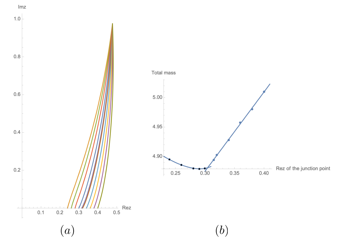
Since the brane configuration is symmetric under the reflection with respect to the real axis, we have numerically computed the contours of mass geodesics from the brane 6 to various crossing points on the real axis (the left panel). The position of the brane 5 is . If the crossing point on the real axis is to the left of the brane 5, the total mass of the string connecting the branes 4 and 6 is twice as the “mass geodesic” length connecting the brane 4 and the crossing point. If, on the other hand, the crossing point is to the right of the brane 5, there arises another -string stretching from the brane 5 to the crossing point, which adds to the total mass. We have shown, in the right panel of FIG.6, the numerical result of the total mass of the string or the string junction for various values of the crossing point.
From this figure we can see that the string crossing at around is the lightest. This string is lighter than any string junction with any crossing (=junction) point. The total mass of a string junction increases linearly as the junction point becomes far away from the brane 5 because of the contribution of the third string stretched from the brane 5.
The Hanany-Witten effect HananyWitten is usually referred to as a transition of an open string into a trivalent string junction, from such as one shown FIG.5(a) to one shown in (b). Since it may be regarded as a phenomenon in which a heavier string junction state becomes lighter than an open string state, we may say that, in the present brane configuration, this effect has not occurred for the string between the branes 4 and 6.
V Orientifold limit in the spectral cover/Higgs bundle approach
In F-theory, the spectral cover describes the vector bundle of the dual heterotic theory FMW; Curio; DiaconescuIonesei; DonagiWijnholt. The coefficients of the defining equation of the spectral cover comprise a weighted projective space bundle, and they can be identified as the Casimir elements of the Lie algebra of the Higgs field BHV; DonagiWijnholt. Each root of the characteristic/spectral cover equation corresponds to a section of a rational elliptic surface (a K3 surface), and hence a weight of the Mordell-Weyl lattice OguisoShioda, which is typically the weight lattice of the Lie algebra of the Higgs.55 5 Very recently, the construction of a K3 surface is generalized to complex-three and -four dimensions with interesting applications to F-theory compactifications Kimura1; Kimura2.
In DonagiWijholtHiggsbundle, the orientifold limit was considered in the spectral cover/Higgs bundle set-up. The Weierstrass equation is taken to be
| (35) |
The discriminant is
| (36) |
In DonagiWijholtHiggsbundle, the leading-order discriminant components are respectively identified as:
| (37) |
Let us confirm this by drawing the dissin.
Fig.7 is the dessin on the base drawn for with on the -plane. Since the discriminant is a cubic polynomial in (as the higher-order terms cancel), we can see three 7-branes, two very close to the origin and one isolated from them at around . The former is to be identified as the O7-plane, whereas the latter is the D7-brane, as is expected in (37). However, they are not the exact discriminant loci but the only approximate values of the 7-brane positions up to . In particular, is not a double zero of the discriminant if we take the corrections into account.
The Fig.8 shows a closer view of the region around . There we can see that the two 7-branes split and form two clusters with an -plane and -plane. If we look more closely at one of the clusters, we can see that the 7-brane sits inside a small area surrounded by -walls.
This is exactly what we have observed in dessinonthebase, Fig.6, where we have also considered a deformation of a fiber in which four D-branes come close together from the rest around the origin. In that case, each of the remaining two D-branes forms a cluster with an -plane and -plane; they are a B-brane and a C-brane, which are regarded as constituent elements of an O7-plane.
VI Conclusions
In this paper we have provided three examples of the use of the new method of describing the non-localness of 7-branes by drawing a “dessin”. The first example was a deformation of the Kodaira fiber. Using the dessin, we were able to immediately recognize which pairs of 7-branes were (non-)local and compute their monodromies. We next solved the mass geodesic equation to examine whether the Hanany-Witten effect occurred in the example. Finally, we considered the orientifold limit in the spectral cover/Higgs bundle approach to observe the characteristic configuration of an O-plane found previously.
A dessin on the base can display which region is strong- or weak-coupling. It shows how the base is covered with such cell regions, which form something like a mosaic in F-theory. In a perturbative string theory, the expectation value of a dilaton is the coupling “constant”, being an expansion parameter in the genus expansion. In a warped compactification like a Randall-Sundrum type model or an AdS/CFT set-up, there are usually only two regions in which the coupling constant is weak or strong. Thus, such a mosaic structure of the coupling constant on the base is very characteristic to F-theory. Moreover, the region encircled by S-walls is a connected region in which one can definitely say that the coupling is weak or strong, but which it is is depending on the frame, i.e. the choice of the fundamental region taken there. A dessin on the base can visualize these special features of F-theory in a clear manner.
The dessin we considered is a map drawn on the base, which is locally homeomorphic to the upper half plane. This is thanks to the special Belyi function, which happened to be defined by the formula of obtaining the modulus via the inverse of the -function. This allows us to know which of the 7-branes are non-local, easily compute the monodromies, and find out whether or not the Hanany-Witten effect has occurred, as we have demonstrated in this paper. We have also found in an orientifold limit in the Higgs bundle approach the characteristic configuration of an O-plane found previously.
We hope that the present analysis will help understanding, from a differential geometrical point of view, the results obtained in the algebrogeometric/gauge theoretic approaches, such as the structures of higher codimension and/or higher-rank enhanced singularities (e,g, HKTW; MorrisonTaylor; BoxGraphs; FtheoryFamilyUnification; MizoguchiTaniAnomaly).
We thank the referee of the journal of our previous paper dessinonthebase for bringing the notion of dessin d’enfant to our attention. We also thank S. Iso, H. Otsuka, K. Sakai and T. Tani for discussions.
References
- (1) A. Grothendieck, “Esquisse d’un Programme”, (1984 manuscript). Published in Schneps and Lochak (1997, I), pp.5-48; English transl., ibid., pp. 243-283. MR1483107.
- (2) S.K.Lando and A.K.Zvonkin, “Graphs on Surfaces and Their Applications, Encyclopaedia of Mathematical Sciences: Lower-Dimensional Topology II”, 141, (2004). Berlin, New York: Springer-Verlag, ISBN 978-3-540-00203-1, Zbl 1040.05001.
- (3) S. Fukuchi, N. Kan, S. Mizoguchi and H. Tashiro, “A dessin on the base: a description of mutually non-local 7-branes without using branch cuts”, [arXiv:1808.04135 [hep-th]]. To appear in Phys. Rev. D.
- (4) T. Tani, Nucl. Phys. B 602 (2001) 434.
- (5) A. Sen, Nucl. Phys. B 475 (1996) 562 [hep-th/9605150].
- (6) N. Seiberg and E. Witten, Nucl. Phys. B 431 (1994) 484 [hep-th/9408099].
- (7) M.R. Gaberdiel, T. Hauer and B. Zwiebach, Open string - string junction transitions, Nucl. Phys. B525 (1998) 117, [hep-th/9801205].
- (8) O. DeWolfe and B. Zwiebach, String Junctions for Arbitrary Lie Algebra Represen- tations, Nucl. Phys. B541 (1999) 509, [hep-th/9804210].
- (9) O. DeWolfe, T. Hauer, A. Iqbal and B. Zwiebach, Adv. Theor. Math. Phys. 3, 1785 (1999) [hep-th/9812028].
- (10) B. R. Greene, A. D. Shapere, C. Vafa and S. T. Yau, Nucl. Phys. B 337 (1990) 1.
- (11) J. H. Schwarz, Phys. Lett. B 360 (1995) 13. Erratum: Phys. Lett. B 364 (1995) 252 [hep-th/9508143].
- (12) A. Sen, Phys. Rev. D 55 (1997) 2501 [hep-th/9608005].
- (13) A. Hanany and E. Witten, Nucl. Phys. B 492, 152 (1997) [hep-th/9611230].
- (14) R. Friedman, J. Morgan and E. Witten, Commun. Math. Phys. 187, 679 (1997) doi:10.1007/s002200050154 [hep-th/9701162].
- (15) G. Curio, Phys. Lett. B 435, 39 (1998) [hep-th/9803224].
- (16) D. E. Diaconescu and G. Ionesei, JHEP 9812, 001 (1998) [hep-th/9811129].
- (17) R. Donagi and M. Wijnholt, Adv. Theor. Math. Phys. 15, 1237 (2011) [arXiv:0802.2969 [hep-th]].
- (18) K. Oguiso and T. Shioda, Comment. Math. Univ. St. Pauli. 40 (1991) 83.
- (19) Y. Kimura, arXiv:1910.00008 [hep-th].
- (20) Y. Kimura, arXiv:1911.03960 [hep-th].
- (21) C. Beasley, J. J. Heckman and C. Vafa, JHEP 0901, 058 (2009) [arXiv:0802.3391 [hep-th]].
- (22) R. Donagi and M. Wijnholt, Commun. Math. Phys. 326 (2014) 287 [arXiv:0904.1218 [hep-th]].
- (23) H. Hayashi, T. Kawano, R. Tatar and T. Watari, Nucl. Phys. B 823 (2009) 47 [arXiv:0901.4941 [hep-th]].
- (24) D. R. Morrison and W. Taylor, JHEP 1201, 022 (2012) [arXiv:1106.3563 [hep-th]].
- (25) H. Hayashi, C. Lawrie, D. R. Morrison and S. Schafer-Nameki, JHEP 1405 (2014) 048 [arXiv:1402.2653 [hep-th]].
- (26) S. Mizoguchi, JHEP 1407 (2014) 018 [arXiv:1403.7066 [hep-th]].
- (27) S. Mizoguchi and T. Tani, PTEP 2016 (2016) no.7, 073B05 [arXiv:1508.07423 [hep-th]].