On the Habitable Lifetime of Terrestrial Worlds with High Radionuclide Abundances
Abstract
The presence of a liquid solvent is widely regarded as an essential prerequisite for habitability. We investigate the conditions under which worlds outside the habitable zones of stars are capable of supporting liquid solvents on their surface over geologically significant timescales via combined radiogenic and primordial heat. Our analysis suggests that super-Earths with radionuclide abundances that are times higher than Earth can host long-lived water oceans. In contrast, the requirements for long-lived ethane oceans, which have been explored in the context of alternative biochemistries, are less restrictive: relative radionuclide abundances of could be sufficient. We find that this class of worlds might be detectable ( detection over days integration time at m) in principle by the James Webb Space Telescope at distances of pc if their ages are Gyr.
I Introduction
Due to the rapid growth of exoplanetary science, there has been renewed interest in determining the conditions that render a planet habitable (Kasting 2012; Lingam & Loeb 2019a). One of the most widely used criteria for habitability is the existence of a suitable liquid solvent, based on which the concept of the habitable zone (HZ) was introduced. The HZ is defined as the region around the host star where liquid water can theoretically exist on the planet’s surface (Dole 1964; Kasting et al. 1993; Ramirez 2018; Ramirez et al. 2019). It is, however, crucial to recognize that habitability is a broader concept than the HZ, implying that worlds outside the HZ may be habitable.
It is expected that worlds beyond the HZ outnumber those in the HZ by orders of magnitude (Lingam & Loeb 2019b). The most widely studied class of potentially habitable worlds beyond the HZ, motivated by the likes of Europa and Enceladus in our Solar system, is icy worlds with subsurface oceans (Nimmo & Pappalardo 2016). Along similar lines, it has been proposed that carbonaceous asteroids and Kuiper belt objects could also be abodes for life (Abramov & Mojzsis 2011). Looking even farther afield, free-floating planets might also be capable of hosting life, especially in subsurface environments (Stevenson 1999; Badescu 2011; Abbot & Switzer 2011; Lingam & Loeb 2019b). In many of these cases, the heating necessary for sustaining liquid solvents is derived from radioactivity, which is sensitive to the age of the world under consideration.
In this Letter, we investigate the role of primordial and radiogenic heating in sustaining liquid solvents on the surface as a function of the size, age and radionuclide abundances of the objects. Unlike most previous studies, we will analyze the prospects for multiple solvents because there are no definitive grounds for supposing that water is the only solvent capable of hosting life (Schulze-Makuch & Irwin 2018). We also study the prospects for their detectability via JWST.
II Contributions to surface heat flux
The current heat flow to Earth’s surface is generated by radiogenic decay and primordial heat from Earth’s formation (Melosh 2011). We can likewise estimate the corresponding heat fluxes for other worlds. Before doing so, we note that the total radiogenic surface heat flux () is estimated via
| (1) |
where denotes the age of the world, whereas and represent the initial radioactive heat flux (at ) and characteristic decay timescale of the element, respectively. In our subsequent analysis, we will address short- and long-lived radionuclides separately and focus on the dominant isotopes.11 1 A third category (“medium-life” isotopes), comprising the likes of plutonium-244 ( Myr) and lead-205 ( Myr), may have to be included for certain stellar systems (Lugaro et al. 2018). For Solar system analogs, however, the conventional division into short- and long-lived nuclides is sufficient.
First, we consider the contribution from the decay of long-lived radionuclides such as uranium-238 and thorium-232. The radiogenic heating rate (in W) is usually modeled as being proportional to the mass of the world; this amounts to assuming that the heating rate per unit mass (units of W/kg) is constant. Using this scaling in conjunction with the mass-radius relationship (Zeng et al. 2016), the radiogenic heat flux associated with long-lived radionuclides () is
| (2) |
where represents the characteristic timescale for the decay of long-lived radionuclides and measures the abundance of radionuclides per unit mass relative to the Earth. In obtaining this formula, we used the fact that radionuclide concentration exhibits exponential decay along with the scaling . Although the magnitude of depends on the specific composition of the world under consideration, we will adopt Gyr for Earth-like worlds (see Section 6.24 of Turcotte & Schubert 2002). The normalization has been chosen such that we obtain a heat flux of for modern Earth (The KamLAND Collaboration 2011).
The next major contribution is the primordial heat released as the world cools after its formation. The surface heat flux arising from this activity () is estimated from Eq. (7.200) of Turcotte & Schubert 2002:
| (3) |
where is the mean specific heat, denotes the mean mass density and signifies the average rate of mantle cooling. By using the scaling , we find that . Estimating the temporal dependence of is complicated because it depends on several mantle properties, but we will suppose that it can be heuristically modeled using Eq. (7.211) of Turcotte & Schubert 2002:
| (4) |
where is a composite variable that depends solely on the radionuclide composition and rheology of the mantle; however, it does not depend on the mantle thickness, its fiducial viscosity and current rate of heat generation. As our analysis deals with rocky worlds akin to Earth, we will hold , where K-1 yr-1 is the value for Earth (Turcotte & Schubert 2002). After solving the above differential equation and substituting the expression into (3), we arrive at
| (5) |
where Gyr is the Earth’s current age; the normalization factor preserves consistency with present-day Earth (The KamLAND Collaboration 2011).
Although and represent the dominant long-term contributions to the surface heat flow, it is important to recognize that short-lived radionuclides can contribute to brief, but intense, initial heating (Hevey & Sanders 2006; Abramov & Mojzsis 2011). Although a number of short-lived radionuclides exist, the most notable among them are iron-60 and aluminium-26, but we shall concentrate on the latter due to its relatively higher abundance in planetesimals of the early Solar system (Lichtenberg et al. 2016). The heat flux associated with this short-lived radionuclide () is obtained by following the derivation that led to (2), thereby yielding
| (6) |
where Myr, measures the abundance of aluminium-26 relative to early Solar system planetesimals, and the normalization constant follows upon utilizing the heat generation per unit mass (Abramov & Mojzsis 2011); this derivation assumed that the world is primarily composed of rocky material.
The total heat flux () is given by the sum of the various contributions, i.e., we have
| (7) |
We are now in a position to estimate the effective temperature () using the Stefan–Boltzmann law:
| (8) |
At this stage, it is important to recognize that is not only dependent on the age of the world but also on its mass as well as and . In order to simplify the problem, we will presume that the relative abundances of short- and long-lived radionuclides are equal to each other, i.e., we specify .
III Surface temperature and habitability duration
Our goal is to determine the duration of surface habitability, i.e., the length of time over which a liquid solvent can exist on the surface. There are two points that need to be underscored at this juncture. First, we do not address the prospects for subsurface habitability in this work. The primary reason is that subsurface biospheres are virtually impossible to detect at interstellar distances, even if they emit plumes (Lingam & Loeb 2019b). The temperature in the interior () can be calculated by solving the heat transfer equation (see Eq. (4.13) of Melosh 2011):
| (9) |
where is the heat capacity at constant pressure, is the heating rate per unit mass, and is the thermal diffusivity; the time-dependent boundary condition for this PDE is set by , where is the surface temperature. We will not solve this PDE because it pertains to subsurface habitable conditions.
The second issue concerns the atmosphere, which permits the solvent to exist in liquid form on the surface. Massive and optically thick atmospheres have the capacity to mitigate cooling and thereby retain potentially habitable surface conditions for long timescales (Stevenson 1999; Badescu 2011). We shall, instead, adopt the conservative choice of tenuous and optically thin atmospheres for several reasons. For starters, the habitability timescale herein constitutes a lower bound as explained above. In addition, biosignatures in thick atmospheres dominated by hydrogen and other reducing gases have not been widely modeled. Lastly, the retention of massive atmospheres over long timescales might prove to be difficult for some rocky worlds (Dong et al. 2017; Lingam & Loeb 2019a). For sufficiently tenuous atmospheres, the surface temperature () is approximated by hereafter. Our results for the habitability lifetime are not very sensitive to the optical depth if it is much smaller than unity.
To complete our analysis, it is necessary to choose appropriate solvents. A number of compounds apart from water have been identified as viable candidates for biochemical reactions to occur. We choose ammonia, an inorganic polar solvent, because it has been the subject of several experimental studies (Schulze-Makuch & Irwin 2018). We adopt ethane, an organic polar solvent, on account of its presumed commonality and its potential to harbor alternative biochemistries (Ballesteros et al. 2019). For a surface pressure of bar, water, ammonia and ethane are liquids between K to K, K to K and K to K, respectively. The surface temperature as a function of time is determined from (8), and the above ranges are employed to estimate the habitability timescale ().
Fig. 1 depicts the surface temperature for and different choices of . It is apparent that has a major impact on . For , we find that neither water nor ammonia oceans are feasible, although ethane oceans can persist for Myr. In contrast, for , short-lived water and ammonia oceans may exist for Myr, but ethane oceans are capable of surviving for several Gyr. Lastly, when it comes to , we observe that both water and ammonia oceans are feasible over Gyr timescales.
Next, we examine the role of the object’s mass. From (7) and (8), the ensuing scaling is , thus suggesting that both and should have a weak dependence on . In actuality, exhibits a complex relationship with due to the co-dependence on . This becomes evident upon inspecting Fig. 2, where while is varied. For , we observe that water and ammonia oceans can exist for only Myr. In contrast, for , these oceans could persist over Gyr timescales.
IV Discussion and Conclusions
Finally, we will briefly discuss some implications for biology and feasibility of detection.
IV.1 Biological implications
We do not have a clear picture of when life originated on Earth, under the implicit assumption that it was not transported via panspermia. As per the latest phylogenetic and paleontological evidence, allied to theoretical arguments, there are tentative grounds for supposing that abiogenesis occurred Myr after Earth’s formation (Lazcano & Miller 1994; Dodd et al. 2017; Betts et al. 2018). It is important, however, to recognize that we have no knowledge of the timescale for abiogenesis on other worlds (Spiegel & Turner 2012). In addition, the process of terrestrial planet formation from the protoplanetary disk may necessitate - Myr (Morbidelli et al. 2012; Armitage 2018).
Based on the above arguments, it would seem desirable for to exceed Myr in order for life to originate. If the pace of evolution is similar to that on Earth, the manifestation of detectable biosignatures engendered by microbes might require Gyr. Thus, in order for - Gyr to be realized, Figs. 1 and 2 suggest that and are necessary. This immediately raises the question of whether such high concentrations of long-lived radionuclides are attainable, and by what pathways they can occur.
Before tackling this issue, a comment on potential microbial ecosystems is in order. Although radioactivity levels will indubitably be high on these worlds, many Earth-based extremophiles (e.g., Deinococcus radiodurans) readily tolerate high doses. In fact, the chemoautotrophic bacterium Desulforudis audaxviator derives its energy requirements indirectly from radioactivity (Chivian et al. 2008). The surface heat flux is - W/m2 when conditions suitable for liquid water exist. Of this energy flux, only a small fraction will be accessible to perform work due to thermodynamic constraints (Lingam & Loeb 2019c). Nevertheless, even if merely of the total flux is utilized, it is still orders of magnitude higher than the basal requirement of W/m2 imposed by metabolism (Kempes et al. 2017); it is also two orders of magnitude higher than the energy flux required by Chlorobiaceae in the Black Sea (Manske et al. 2005).
Now, we examine the abundances of long-lived radionuclides. Analysis of near-infrared signatures has revealed that r-process elements (which include uranium and thorium) are predominantly synthesized during neutron star mergers (Kasen et al. 2017; Kajino et al. 2019).22 2 https://blog.sdss.org/wp-content/uploads/2017/01/periodic_table.png Thus, if the rate of neutron star mergers per unit volume tracks the stellar density, it is conceivable that worlds in the inner regions of the Galactic bulge or in environments that are gas-poor (e.g., in elliptical galaxies) could exhibit higher radionuclide concentrations; furthermore, many metal-poor stars with enriched r-process elements have been detected (Frebel 2018).
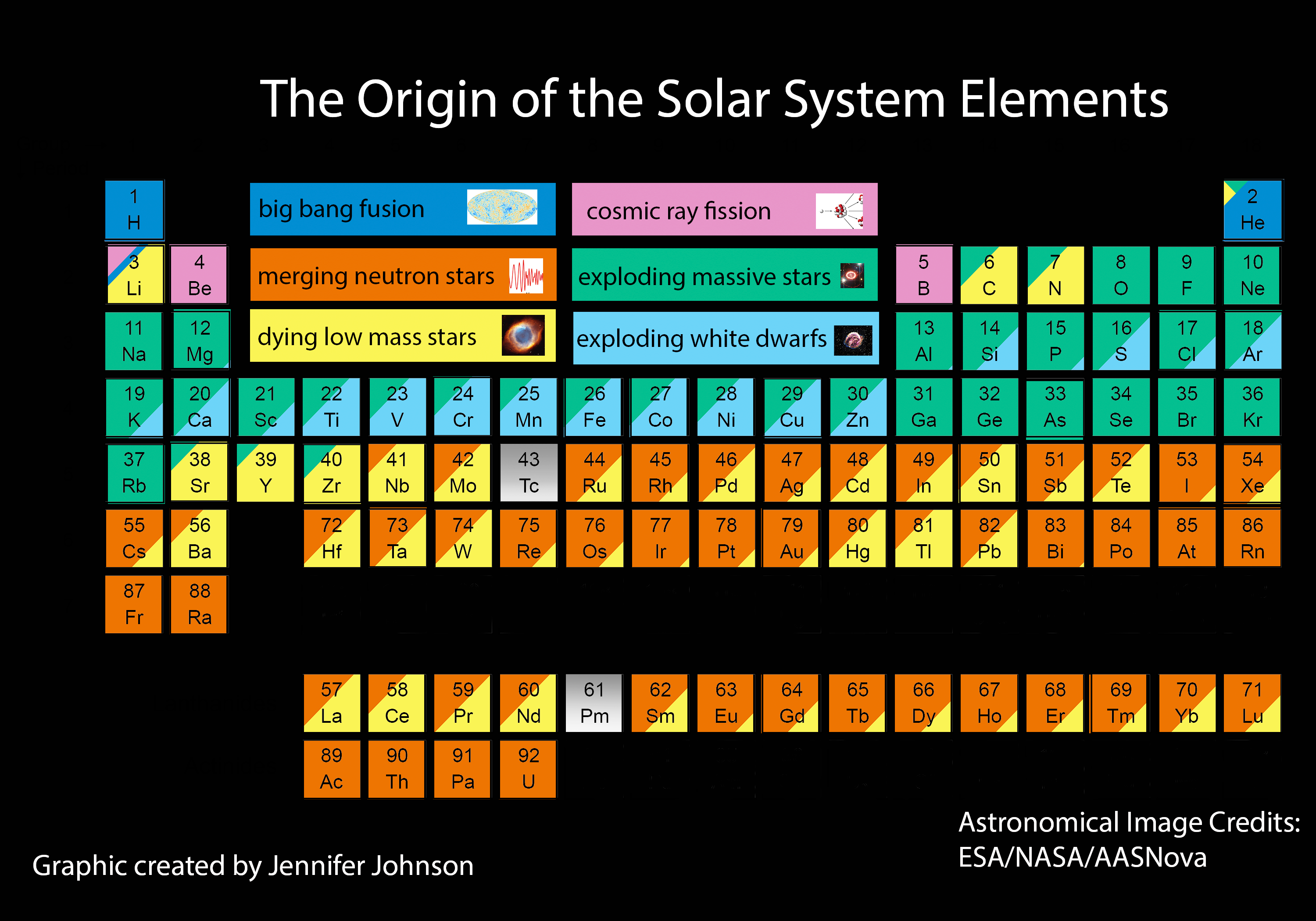
Spectroscopic surveys of solar twins and analogs have shown that the solar abundance of thorium is a few times lower () than other stars in the sample (Unterborn et al. 2015; Botelho et al. 2019). Overall, some worlds will be characterized by elevated abundances of long-lived radionuclides (Lugaro et al. 2018). Turning our attention to short-lived radionuclides, specifically aluminium-26, they are unlikely to affect habitability over Gyr timescales, irrespective of their initial inventory. However, a number of crucial short-term factors depend on its abundance such as differentiation and dehydration of planetesimals (Gilmour & Middleton 2009; Lichtenberg et al. 2019), and melting ice to initiate serpentinization (Góbi & Kereszturi 2017). A number of metrics indicate that high levels of aluminium-26 are widespread in extrasolar systems, especially in young stars (Lugaro et al. 2018).
The situation is rendered quite different when we consider oceans of liquid ethane. For super-Earths with relatively modest enhancements of , we find that - Gyr is realizable. Due to the relatively weaker constraints on , the existence of long-lived ethane oceans is more plausible with respect to water oceans; for different reasons, Ballesteros et al. 2019 concluded that ethane seas may be the most common in the Universe. Thus, there exist compelling grounds to investigate potential biochemistries in liquid ethane as well as the resultant biosignatures.
If habitable conditions persist for Myr, another factor must be taken into consideration for free-floating worlds. Due to the relative motion of stars as well as their ejection from the parent stellar system, they ought to have typical velocities of km/s with respect to nearby stars. Thus, over a period of Myr, they can traverse distances of kpc. During the course of this journey, they may be captured by three-body gravitational interactions into binary systems (Ginsburg et al. 2018). Once they have been captured, this opens the possibility of seeding other worlds in that system via interplanetary panspermia.33 3 Note that the prospects for interplanetary panspermia are enhanced for clustered planetary systems such as those around M-dwarfs (Lingam & Loeb 2017).
IV.2 Detectability of objects
In order to detect worlds that are rendered habitable by radiogenic and primordial heating, the spectral flux density () received at Earth via black body emission must be sufficiently high (see Abbot & Switzer 2011).44 4 In some respects, our analysis is similar to the detection of free-floating Y-type brown dwarfs (Burrows et al. 2003; Biller 2017), because they have black body temperatures as low as K. is determined by scaling the black body spectral radiance of the object as follows:
| (10) |
where is the Planck function, is the frequency and is the distance of the object from Earth. We adopt a wavelength of m, for which the sensitivity of the imager corresponding to the Mid-Infrared Instrument (MIRI) instrument on board JWST is Jy to achieve detection over s of integration time (see Table 2 of Rieke et al. 2015).55 5 https://www.jwst.nasa.gov/ Hence, over an integration time of s (viz., days), the detection threshold would be lowered to nJy. At this wavelength, the above expression can be rewritten to yield
| (11) |
Due to the exponential dependence of on , will naturally be very sensitive to the age, radionuclide abundance and mass of the object.
Figs. 3 and 4 depict for the fiducial choices of m and pc. For relatively high radionuclide abundances () and high masses (), we find that the MIRI instrument may detect such worlds provided they are Gyr old. In contrast, objects with lower values of and are unlikely to be detectable by MIRI unless they are located relatively close to Earth. Based on available estimates for the density of free-floating planets, Lingam & Loeb 2019b suggested that the distance to the nearest roughly Mars-sized free-floating object might be on the order of pc. In this case, objects with are potentially detectable by MIRI during the first Myr of their existence, while could boost detectability to Gyr timescales.
Hence, in principle, planets with sufficiently high abundances that are relatively nearby might remain detectable over long timescales. A number of young stellar comoving groups have been detected at distances of - pc from Earth with stellar ages of - Myr (Zuckerman & Song 2004). Examples of such groups include the Pictoris moving group (Mamajek & Bell 2014) and the TW Hydrae association (Ducourant et al. 2014; Gagné et al. 2017), whose median ages are Myr and Myr, respectively. If worlds far removed from the HZs of such stars are characterized by and sufficiently high radionuclide abundances, they may fulfill the requirements for detectability by JWST based on Figs. 3 and 4.
In the event that JWST detects either a free-floating object or one that is far beyond the HZ with an anomalously high temperature (and thin atmosphere), one can use to place constraints on its age and radionuclide abundance. For such worlds, thermal emission spectroscopy could be utilized to discern potential atmospheric biosignatures (Fujii et al. 2018).
References
- Abbot & Switzer (2011) Abbot, D. S., & Switzer, E. R. 2011, Astrophys. J. Lett., 735, L27, doi: 10.1088/2041-8205/735/2/L27
- Abramov & Mojzsis (2011) Abramov, O., & Mojzsis, S. J. 2011, Icarus, 213, 273, doi: 10.1016/j.icarus.2011.03.003
- Armitage (2018) Armitage, P. J. 2018, A Brief Overview of Planet Formation, ed. H. J. Deeg & J. A. Belmonte (Springer), 2185–2203, doi: 10.1007/978-3-319-55333-7_135
- Badescu (2011) Badescu, V. 2011, Icarus, 216, 485, doi: 10.1016/j.icarus.2011.09.013
- Ballesteros et al. (2019) Ballesteros, F. J., Fernandez-Soto, A., & Martínez, V. J. 2019, Astrobiology, 19, 642, doi: 10.1089/ast.2017.1720
- Betts et al. (2018) Betts, H. C., Puttick, M. N., Clark, J. W., et al. 2018, Nat. Ecol. Evol., 2, 1556, doi: 10.1038/s41559-018-0644-x
- Biller (2017) Biller, B. 2017, Astron. Rev., 13, 1, doi: 10.1080/21672857.2017.1303105
- Botelho et al. (2019) Botelho, R. B., Milone, A. d. C., Meléndez, J., et al. 2019, Mon. Not. R. Astron. Soc., 482, 1690, doi: 10.1093/mnras/sty2791
- Burrows et al. (2003) Burrows, A., Sudarsky, D., & Lunine, J. I. 2003, Astrophys. J., 596, 587, doi: 10.1086/377709
- Chivian et al. (2008) Chivian, D., Brodie, E. L., Alm, E. J., et al. 2008, Science, 322, 275, doi: 10.1126/science.1155495
- Dodd et al. (2017) Dodd, M. S., Papineau, D., Grenne, T., et al. 2017, Nature, 543, 60, doi: 10.1038/nature21377
- Dole (1964) Dole, S. H. 1964, Habitable planets for man (Blaisdell Pub. Co.)
- Dong et al. (2017) Dong, C., Lingam, M., Ma, Y., & Cohen, O. 2017, Astrophys. J. Lett., 837, L26, doi: 10.3847/2041-8213/aa6438
- Ducourant et al. (2014) Ducourant, C., Teixeira, R., Galli, P. A. B., et al. 2014, Astron. Astrophys., 563, A121, doi: 10.1051/0004-6361/201322075
- Frebel (2018) Frebel, A. 2018, Annu. Rev. Nucl. Part. Sci., 68, 237, doi: 10.1146/annurev-nucl-101917-021141
- Fujii et al. (2018) Fujii, Y., Angerhausen, D., Deitrick, R., et al. 2018, Astrobiology, 18, 739, doi: 10.1089/ast.2017.1733
- Gagné et al. (2017) Gagné, J., Faherty, J. K., Mamajek, E. E., et al. 2017, Astrophys. J. Suppl., 228, 18, doi: 10.3847/1538-4365/228/2/18
- Gilmour & Middleton (2009) Gilmour, J. D., & Middleton, C. A. 2009, Icarus, 201, 821, doi: 10.1016/j.icarus.2009.03.013
- Ginsburg et al. (2018) Ginsburg, I., Lingam, M., & Loeb, A. 2018, Astrophys. J. Lett., 868, L12, doi: 10.3847/2041-8213/aaef2d
- Góbi & Kereszturi (2017) Góbi, S., & Kereszturi, Á. 2017, Mon. Not. R. Astron. Soc., 466, 2099, doi: 10.1093/mnras/stw3223
- Hevey & Sanders (2006) Hevey, P. J., & Sanders, I. S. 2006, Meteorit. Planet. Sci., 41, 95, doi: 10.1111/j.1945-5100.2006.tb00195.x
- Kajino et al. (2019) Kajino, T., Aoki, W., Balantekin, A. B., et al. 2019, Prog. Part. Nucl. Phys., 107, 109, doi: 10.1016/j.ppnp.2019.02.008
- Kasen et al. (2017) Kasen, D., Metzger, B., Barnes, J., Quataert, E., & Ramirez-Ruiz, E. 2017, Nature, 551, 80, doi: 10.1038/nature24453
- Kasting (2012) Kasting, J. 2012, How to Find a Habitable Planet (Princeton University Press)
- Kasting et al. (1993) Kasting, J. F., Whitmire, D. P., & Reynolds, R. T. 1993, Icarus, 101, 108, doi: 10.1006/icar.1993.1010
- Kempes et al. (2017) Kempes, C. P., van Bodegom, P. M., Wolpert, D., et al. 2017, Front. Microbiol., 8, 31, doi: 10.3389/fmicb.2017.00031
- Lazcano & Miller (1994) Lazcano, A., & Miller, S. L. 1994, J. Mol. Evol., 39, 546, doi: 10.1007/BF00160399
- Lichtenberg et al. (2019) Lichtenberg, T., Golabek, G. J., Burn, R., et al. 2019, Nat. Astron., 3, 307, doi: 10.1038/s41550-018-0688-5
- Lichtenberg et al. (2016) Lichtenberg, T., Golabek, G. J., Gerya, T. V., & Meyer, M. R. 2016, Icarus, 274, 350, doi: 10.1016/j.icarus.2016.03.004
- Lingam & Loeb (2017) Lingam, M., & Loeb, A. 2017, Proc. Natl. Acad. Sci., 114, 6689, doi: 10.1073/pnas.1703517114
- Lingam & Loeb (2019a) —. 2019a, Rev. Mod. Phys., 91, 021002, doi: 10.1103/RevModPhys.91.021002
- Lingam & Loeb (2019b) —. 2019b, Int. J. Astrobiol., 18, 112, doi: 10.1017/S1473550418000083
- Lingam & Loeb (2019c) —. 2019c, Astrophys. J., 883, 143, doi: 10.3847/1538-4357/ab3f35
- Lugaro et al. (2018) Lugaro, M., Ott, U., & Kereszturi, Á. 2018, Prog. Part. Nucl. Phys., 102, 1, doi: 10.1016/j.ppnp.2018.05.002
- Mamajek & Bell (2014) Mamajek, E. E., & Bell, C. P. M. 2014, Mon. Not. R. Astron. Soc., 445, 2169, doi: 10.1093/mnras/stu1894
- Manske et al. (2005) Manske, A. K., Glaeser, J., Kuypers, M. M. M., & Overmann, J. 2005, Appl. Environ. Microbiol., 71, 8049, doi: 10.1128/AEM.71.12.8049-8060.2005
- Melosh (2011) Melosh, H. J. 2011, Planetary Surface Processes (Cambridge University Press)
- Morbidelli et al. (2012) Morbidelli, A., Lunine, J. I., O’Brien, D. P., Raymond, S. N., & Walsh, K. J. 2012, Annu. Rev. Earth Planet. Sci., 40, 251, doi: 10.1146/annurev-earth-042711-105319
- Nimmo & Pappalardo (2016) Nimmo, F., & Pappalardo, R. T. 2016, J. Geophys. Res. E, 121, 1378, doi: 10.1002/2016JE005081
- Ramirez et al. (2019) Ramirez, R., Abbot, D. S., Fujii, Y., et al. 2019, in Bulletin of the American Astronomical Society, Vol. 51, 31
- Ramirez (2018) Ramirez, R. M. 2018, Geosciences, 8, 280, doi: 10.3390/geosciences8080280
- Rieke et al. (2015) Rieke, G. H., Wright, G. S., Böker, T., et al. 2015, Publ. Astron. Soc. Pac, 127, 584, doi: 10.1086/682252
- Schulze-Makuch & Irwin (2018) Schulze-Makuch, D., & Irwin, L. N. 2018, Life in the Universe: Expectations and Constraints, 3rd edn. (Springer), doi: 10.1007/978-3-319-97658-7
- Spiegel & Turner (2012) Spiegel, D. S., & Turner, E. L. 2012, Proc. Natl. Acad. Sci. USA, 109, 395, doi: 10.1073/pnas.1111694108
- Stevenson (1999) Stevenson, D. J. 1999, Nature, 400, 32, doi: 10.1038/21811
- The KamLAND Collaboration (2011) The KamLAND Collaboration. 2011, Nat. Geosci., 4, 647, doi: 10.1038/ngeo1205
- Turcotte & Schubert (2002) Turcotte, D. L., & Schubert, G. 2002, Geodynamics, 2nd edn. (Cambridge University Press)
- Unterborn et al. (2015) Unterborn, C. T., Johnson, J. A., & Panero, W. R. 2015, Astrophys. J., 806, 139, doi: 10.1088/0004-637X/806/1/139
- Zeng et al. (2016) Zeng, L., Sasselov, D. D., & Jacobsen, S. B. 2016, Astrophys. J., 819, 127, doi: 10.3847/0004-637X/819/2/127
- Zuckerman & Song (2004) Zuckerman, B., & Song, I. 2004, Annu. Rev. Astron. Astrophys., 42, 685, doi: 10.1146/annurev.astro.42.053102.134111