Tilings from Graph Directed Iterated Function Systems

Michael Barnsley and Andrew Vince Address: Mathematical Sciences Institute, Australian National University, Canberra, ACT, Australia
michael.barnsley@anu.edu.au Address: Department of Mathematics, University of Florida, Gainesville, FL, USA
avince@ufl.edu

Abstract.

A new method for constructing self-referential tilings of Euclidean space from a graph directed iterated function system, based on a combinatorial structure we call a pre-tree, is introduced. In the special case that we refer to as balanced, the resulting tilings have a finite set of prototiles, are quasiperiodic but not periodic, and are self-similar. A necessary and sufficient condition for two balanced tilings to be congruent is provided.

Key words and phrases:

tiling, graph directed iterated function system, self-similar

2020 Mathematics Subject Classification

52C20, 52C22, 05B45, 28A80

1. Introduction

Iterated function systems (IFSs) have been at the heart of fractal geometry almost from its origins, and the attractor $A$ of the IFS has played the central role in the theory. The attractor is the union of contracted images of itself. In the case that the contractions are similarities, the attractor is the union of smaller similar copies of itself. See [14] for formal background on iterated function systems (IFS). Here we are concerned with a generalization of an IFS, called a graph directed iterated function system (GIFS). A GIFS generalizes the IFS concept so that the attractor has components $A_{1},A_{2},\dots,A_{n}$ , each component $A_{i}$ the union of contracted copies of the components $A_{1},A_{2},\dots,A_{n}$ . The prescription for how this is done is encoded in a directed graph (with possibly multiple edges and loops), the precise definition of a GIFS given in Section 2.1. An IFS is the special case of a GIFS in which the digraph has a single vertex. Early work related to GIFSs includes [3, 4, 7, 8, 9, 18, 26]. In some of these works, a graph IFS are referred to as a recurrent IFS.

The paper [5] introduced a method for constructing certain tilings using an IFS, in which the tiles are related to the attractor of the IFS. This construction included, as special cases, digit tilings [25] (see the right panel of Figure 1 for the twin dragon tiling), crystallographic tilings [12], certain substitution tilings like the “chair tiling” (see the left panel of Figure 1), and new tilings (see, for example, Figure 2). In [6] this method was engineered to obtain tilings of Euclidean space having the properties of repetitivity (quasiperiodicity) and self-similarity (whose definitions appear later in this introduction). In these tilings there are finitely many tiles up to congruence, and all tiles are similar to the attractor of the IFS (see Figure 3).

Refer to caption — Figure 1. the chair tiling and the twin dragon tiling.

The goal of this paper is twofold. First, using a GIFS, we introduce a new unifying method for the construction of tilings of ${\mathbb{R}}^{d}$ . The method is based on a combinatorial structure in the underlying directed graph that we call a pre-tree. This notion is defined precisely in Definition 3 in Section 3.1. Our point of view is more graph theoretic than is usual in papers on fractals via iterated function systems; so for basic notions about graphs see [10]. The approach in this paper is a substantial extension of some concepts in [5] and [6]. Other papers which relate to the use of GIFS to construct tilings include [3, 16, 17].

A given GIFS has infinitely many parameters, the term parameter defined in Section 4.1, and for each parameter ${\overleftarrow{\theta}}$ , many possible ${\overleftarrow{\theta}}$ -sequences $\mathcal{S}$ (see Definition 4 of ${\overleftarrow{\theta}}$ -sequences in Section 3.2). The main result in the first part of the paper is that, for a given GIFS and for each parameter ${\overleftarrow{\theta}}$ and each corresponding ${\overleftarrow{\theta}}$ -sequence $\mathcal{S}$ , there is a tiling $T({\overleftarrow{\theta}},\mathcal{S})$ of Euclidean space (see Theorem 3 in Section 4.2). Addresses can be assigned in a natural way to the tiles in $T({\overleftarrow{\theta}},\mathcal{S})$ as described in Section 4.4. In addition to the tiling examples mentioned in the paragraph above, these GIFS tilings include the Penrose and Rauzy tilings [21], and many others; see, for example, Figures 4, 5 and 9.

Although the tilings constructed by our general method possess a replicating pattern, particularly nice properties are obtained by carefully choosing the ${\overleftarrow{\theta}}$ -sequences. We call such special ${\overleftarrow{\theta}}$ -sequences and the corresponding tilings balanced (see Definition 5 in Section 3.2 and Definition 7 in Section 4.3). The second goal of this paper is to use the balanced property to construct tilings $T$ that satisfy the following properties:

•

$T$ has finitely many tiles up to congruence;
•

$T$ is self-similar;
•

$T$ is repetitive, but not periodic;
•

for a given GIFS, there are uncountably many tilings up to isometry (each associated with a particular parameter).

Note that the tiles do not have to be pairwise similar. The relevant definitions are:

Definition 1.

A tiling $T$ is repetitive, also called quasiperiodic, if, for every finite patch $P$ of $T$ , there is a real number $R$ such that every ball of radius $R$ contains a patch isometric (congruent) to $P$ .

Definition 2.

A tiling $T$ is self-similar if there exists a similarity transformation $\phi:{\mathbb{R}}^{d}\rightarrow{\mathbb{R}}^{d}$ with scaling ratio greater than $1$ such that, for every tile $t\in T$ , its image $\phi(t)$ is, in turn, tiled by tiles in $T$ .

Figures 1 (left panel), 3, 4, 5, and 11 are examples of such balanced tilings. Note that the tiles used in Figures 4, 5 and 11 are not pairwise similar. Work on self-similar tilings has been extensive over the past few decades, dating back at least to the Penrose tilings [19], popularized by M. Gardner [11]. Much recent research was motivated by W. Thurston’s notes [24]. Some formative papers include [2, 13, 15, 20, 23, 25].

Among the main results of the second part of the paper are that the constructed balanced tilings indeed satisfy the above bulleted properties. Many of the proofs, which appear in Section 6, rely heavily on the hierarchical properties of the tilings, as described in Section 5. The tiling map ${\overleftarrow{\theta}}\mapsto T({\overleftarrow{\theta}})$ is a continuous map from the parameter space, as defined in Section 4.1, to the tiling space, as defined in Section 5.2. Theorem 4 states that the shift map on the parameter space corresponds via this tiling map to going up one level in the tiling hierarchy in the tiling space. There is an easily defined equivalence relation on the parameter space (see Definition 13 in Section 6.4) such that the tiling map induces a bijection between the set of parameters up to equivalence and the set of balanced tilings up to congruence (isometry); see Theorem 8 in Section 6.4. This provides a necessary and sufficient condition for two balanced tilings to be congruent.

2. Graph Directed Iterated Function Systems

2.1. GIFS

Let $\mathbb{N}$ denote the set of positive integers, and for $n\in\mathbb{N}$ , let $[n]:=\{1,2,\dots,n\}$ . Let $G=\left(V,E\right)$ be a finite strongly connected directed graph with vertex set $V=[n]$ and edge set $E$ . Strongly connected means that, for any two vertices $i$ and $j$ , there is a directed path from $i$ to $j$ . The digraph $G$ may have loops and/or multiple edges. For an edge $e=(i,j)$ , directed from vertex $i$ to vertex $j$ , the vertex $j$ is called the head, denoted $e^{+}$ , and the vertex $i$ is called the tail, denoted $e^{-}$ . Let $E_{i}$ denote the set of all edges whose tail is $i$ .

In this paper, a path always means a directed path, and a path can have repeated vertices and edges. An infinite path has a starting vertex but no terminal vertex. A path $\sigma=\sigma_{1}\,\sigma_{2}\,\cdots$ will be written as its ordered string of edges $\sigma_{i}\in E,\;i=1,2\dots$ . The starting vertex of a path $\sigma$ will be denoted $\sigma^{-}$ , and the terminal vertex of a finite path by $\sigma^{+}$ . The length of a finite path $\sigma$ , i.e., the number of edges, will be denoted $|\sigma|$ . We allow paths of length zero, consisting of a single vertex.

To each directed edge $e\in E$ of the digraph $G$ , associate a function $f_{e}:{\mathbb{R}}^{d}\rightarrow{\mathbb{R}}^{d}$ . Let

F=\{f_{e}\,:\,e\in E\}.

Each $f\in F$ is assumed throughout this paper to be an invertible contraction. Thus there is a contraction factor $\lambda_{f}<1$ such that $|f(x)-f(y)|\leq\lambda_{f}|x-y|$ for all $f\in F$ and all $x,y\in\mathbb{R}^{d}$ . The pair $(G,F)$ is called a graph directed IFS (GIFS).

Let $\mathbb{H}$ denote the set of nonempty compact subsets of $\mathbb{R}^{d}$ , and define $\mathbf{F}:\mathbb{H}^{n}\rightarrow\mathbb{H}^{n}$ as follows. If $\mathbf{X}=(X_{1},X_{2},\dots,X_{n})\in{\mathbb{H}}^{n}$ , then

\mathbf{F}(\mathbf{X})=\big(F_{1}(\mathbf{X}),F_{2}(\mathbf{X}),\dots,F_{n}(\mathbf{X})\big),

where

F_{i}(\mathbf{X})=\bigcup_{e\in E_{i}}f_{e}(X_{e^{+}}).

Note that, if $G=(V,E)$ and $V$ consists of a single vertex and $E$ is a set of loops, then a graph directed IFS is an ordinary IFS, and $\mathbf{F}$ is the associated Hutchinson operator. Thus a GIFS is a generalization of an IFS.

2.2. Notation

Let $\Sigma^{*}$ denote the set of paths of finite length in the digraph $G$ and $\Sigma^{\infty}$ the set of paths of infinite length. For $\sigma=\sigma_{1}\sigma_{2}\cdots\in\Sigma^{\infty}$ let

\sigma|k=\sigma_{1}\sigma_{2}\cdots\sigma_{k}\in\Sigma^{*},

and $\sigma|0$ the path that is just the vertex $\sigma^{-}$ .

Denote by $\overleftarrow{G}$ the digraph obtained from $G$ by reversing the direction on all edges. Define path spaces $\overleftarrow{\Sigma}^{*}$ and $\overleftarrow{\Sigma}^{\infty}$ accordingly. For any edge $e$ in $G$ , let $\overleftarrow{e}$ be the oppositely directed edge, and define

(2.1)

f_{\overleftarrow{e}}:=(f_{e})^{-1}.

For $\sigma=\sigma_{1}\sigma_{2}\sigma_{3}\cdots\sigma_{k}\in\Sigma^{*}\cup\overleftarrow{\Sigma}^{*}$ , define

(2.2)

f_{\sigma}:=f_{\sigma_{1}}\circ f_{\sigma_{2}}\circ f_{\sigma_{3}}\cdots f_{\sigma_{k}}.

Note that, for $\sigma\in\Sigma^{*}$ , the map $f_{\sigma}$ is a contraction, but for $\sigma\in\overleftarrow{\Sigma}^{*}$ , the map $f_{\sigma}$ is an expansion.

2.3. The Attractor

The following is a standard result in the theory of graph iterated function systems. In the theorem $\mathbf{F}^{k}$ denotes the $k$ -fold iteration of $\mathbf{F}$ .

Theorem 1.

If $\left(G,F\right)$ is a GIFS such that each function in $F$ is a contraction, then there exists a unique $\mathbf{A}=(A_{1},A_{2},...,A_{n})\in\mathbb{H}^{n}$ such that

\mathbf{A=F(A)}

and

\mathbf{A=}\lim_{k\rightarrow\infty}{\mathbf{F}}^{k}(\mathbf{B})

independent of $\mathbf{B}\in\mathbb{H}^{n},$ where convergence is with respect to the Hausdorff metric on $\mathbb{H}^{n}$ .

The above limit formula is equivalent to

(2.3)

A_{i}=\bigcup\big\{\lim_{k\rightarrow\infty}\{f_{\sigma}(B)\,:\,|\sigma|=k,\,\sigma^{-}=i\big\},

for all $i\in[N]$ and for any $B\in\mathbb{H}.$ With notation as in Theorem 1, $\mathbf{A}$ is called the attractor of the GIFS $(G,F)$ and $\left\{A_{i}:i\in[n]\right\}$ is its set of components, each of which is compact. It follows from the definition that, for each $i\in[n]$ , the components of the attractor have the property that

(2.4)

A_{i}=\bigcup_{e\in E_{i}}f_{e}(A_{e^{+}}).

If, for all $i\in[n]$ , the intersection of distinct sets in the union in Equation (2.4) has empty interior, then the attractor $\mathbf{A}$ of the GIFS is said to be non-overlapping. For all GIFSs in this paper we assume that the attractor is non-overlapping and that each component of the attractor has nonempty interior.

3. Pre-Trees and $\theta$ -Sequences

3.1. Pre-Tree

Definition 3.

A subpath of a finite path $\sigma=\sigma_{1}\sigma_{2}\cdots\sigma_{k}$ in a digraph $G$ is defined as a path of the form $\sigma_{1}\sigma_{2}\dots,\sigma_{j}$ , where $0\leq j\leq k$ . (For the case $j=0$ , the subpath consists of a single vertex.) A subpath is called proper if $j<k$ . A set $S$ of finite directed paths in a directed graph is called a pre-tree if

(1)

every path in $S$ begins at the same vertex $r$ , called the root of $S$ ;
(2)

no proper subpath of a path in $S$ lies in $S$ ;
(3)

for every proper subpath $\sigma$ of a path in $S$ and every edge $e\in E$ , if $e^{-}=\sigma^{+}$ , then the path $\sigma e$ is a subpath of a path in $S$ .

The subgraph $\langle S\rangle$ of $G$ consisting of all vertices and edges of $S$ in a pre-tree $S$ may not be a tree. This subgraph $\langle S\rangle$ may contain cycles, even directed cycles. However, there is an actually tree $H(S)$ related to $S$ as described in the following proposition. An example illustrating Proposition 1 and its proof appears in Figure 6.

Graph homomorphism - a map from one graph to another that sends adjacent pairs of vertices to adjacent pairs of vertices - is a standard notion in graph theory. For digraphs with possibly multiple edges and loops, we define a homomorphism from a digraph $G$ to a digraph $G^{\prime}$ as a pair of functions function $h:V(G)\rightarrow V(G^{\prime})$ and $h:E(G)\rightarrow E(G^{\prime})$ such that, if edge $e$ is directed from $i$ to $j$ , then $h(e)$ is directed from $h(i)$ to $h(j)$ . We also use the notation $h:G\rightarrow G^{\prime}$ for a digraph homomorphism.

Proposition 1.

Given a pre-tree $S$ , there is a unique pair consisting of a rooted directed tree $H(S)$ and a homomorphism $h:H(S)\rightarrow\langle S\rangle$ such that

(1)

$h$ takes the root of $H(S)$ to the root of $\langle S\rangle$ ;
(2)

$h$ bijectively maps the set of all paths in $H(S)$ going from the root to a leaf onto $S$ ;
(3)

among all digraphs satisfying properties (1,2), $H(S)$ has the least number of edges.

Proof.

Let $H^{\prime}$ be the rooted tree constructed as follows. The tree $H^{\prime}$ is the union of directed paths $p_{1},p_{2},\dots,p_{m}$ that have one vertex in common, the root. Pairwise these paths in $H^{\prime}$ have no edges in common and no vertices in common except the root. The edges are directed from the root to the leaf. Moreover, these paths are taken to be exactly all the paths in $S$ . See the two left digraphs in Figure 6. Clearly there is a homomorphism $h^{\prime}:H^{\prime}\rightarrow\langle S\rangle$ satisfying properties (1,2).

The rooted directed tree $H(S)$ is obtained from $H^{\prime}$ as a quotient graph. Call two vertices $i,j\in V(H^{\prime})$ equivalent, denoted $i\sim j$ , if there are paths $p_{i}$ and $p_{j}$ in $H^{\prime}$ , from the root to $i$ and $j$ , respectively, such that $p_{i}$ and $p_{j}$ have the same image under $h^{\prime}$ . Call two edges $(i_{1},j_{1})$ and $(i_{2},j_{2})$ in $E(H^{\prime})$ equivalent if $i_{1}\sim i_{2}$ and $j_{1}\sim j_{2}$ . Let $H(S)$ be the tree whose vertices and edges are the equivalence classes of vertices of $H^{\prime}$ . See Figure 6. Define $h:H(S)\rightarrow\langle S\rangle$ by mapping a vertex $v$ to $h^{\prime}(i)$ , where $i\in v$ ; similarly for the image of edges. It is routine to check properties (1-3) and uniqueness. ∎

3.2. $\theta$ -Sequences

Definition 4.

Let $\overleftarrow{\theta}:=\overleftarrow{\theta}_{1}\;\overleftarrow{\theta}_{2}\;\overleftarrow{\theta}_{3}\cdots\in\overleftarrow{\Sigma}^{\infty}$ be an infinite path in $\overleftarrow{G}$ , where $\theta_{i}\in E$ for all $i$ , and let $v_{0},v_{1},v_{2},\dots$ be the successive vertices of ${\overleftarrow{\theta}}$ . An infinite sequence ${\mathcal{S}}=\{S_{0},S_{1},S_{2},\dots\}$ of pre-trees in $G$ is called a $\mathbf{\overleftarrow{\theta}}$ -sequence if, for all $k=0,1,2,\dots,$

(1)

$v_{k}$ is the root of the pre-tree $S_{k}$ , and
(2)

$\theta_{k}\,S_{k-1}:=\{\theta_{k}\sigma:\sigma\in S_{k-1}\}\subset S_{k}$ for all $k\geq 1$ .

The second condition states that the pre-trees along the path ${\overleftarrow{\theta}}$ are, in a sense, nested. Note that edges $\theta_{k}$ and ${\overleftarrow{\theta}}_{k}$ are the same edge oppositely oriented.

3.3. Examples

In the following examples, the directed graph $G$ is given, as well as a path $\overleftarrow{\theta}:=\overleftarrow{\theta}_{1}\;\overleftarrow{\theta}_{2}\;\overleftarrow{\theta}_{3}\cdots\in\overleftarrow{\Sigma}^{\infty}$ with successive vertices $v_{0},v_{1},v_{2},\dots$ . Clearly, numerous examples of ${\overleftarrow{\theta}}$ -sequences can be obtained inductively by choosing an arbitrary pre-tree rooted at $v_{0}$ , then a pre-tree rooted at $v_{1}$ subject to condition (2) in the definition of ${\overleftarrow{\theta}}$ -sequence, and continuing at $v_{2},v_{3},\dots$ . Below, we will give a few specific examples that we return to in Section 4.3.

Example 1.

Let $S_{k},\,k\geq 0,$ be the pre-tree with root $v_{k}$ consisting of all paths of length exactly $k$ . Then ${\mathcal{S}}(\theta)=\{S_{0},S_{1},S_{2},\dots\}$ is a $\overleftarrow{\theta}$ -sequence of pre-trees.

Example 2.

For any $m\in\mathbb{N}$ , let $S_{k},\,k\geq 0,$ be the pre-tree with root $v_{k}$ , where

S_{k}=\{\theta_{k}\theta_{k-1}\cdots\theta_{j+1}\sigma\,:\,0\leq j\leq k,\,\sigma^{-}=v_{j},\;|\sigma|=m\}.

Then ${\mathcal{S}}(\theta,m):=\{S_{0},S_{1},S_{2},\dots\}$ is a $\overleftarrow{\theta}$ -sequence of pre-trees.

In the next examples, assume that $(G,F)$ is a GIFS where each $f\in F$ is a similarity transformation. Such a GIFS will be referred to as a similarity GIFS. For any similarity transformation $f$ , let $\lambda_{f}$ denote the scaling ratio, i.e., $|f(x)-f(y)|=\lambda_{f}\,|x-y|$ for all $x,y\in{\mathbb{R}}^{d}$ .

Example 3.

Given a similarity GIFS, for any pair of positive real numbers $q<Q$ , define a $\overleftarrow{\theta}$ -sequence $\mathcal{S}(\theta,q,Q)=\{S_{0},S_{1},S_{2},\dots\}$ by

S_{k}=\{\sigma\in\Sigma^{*}\,:\,q\leq\lambda(f_{\overleftarrow{\theta}|k})\cdot\lambda(f_{\sigma})\leq Q\}.

Note that, with notation as in equations (2.1) and (2.2) in Section 2.2, the function $f_{\sigma}$ is a contraction, while $f_{\overleftarrow{\theta}|k}$ is an expansion. It is routine to check that condition (3) in the definition of pre-tree and condition (2) in the definition of ${\overleftarrow{\theta}}$ -sequence are satisfied. Therefore ${\mathcal{S}}(\theta,q,Q)$ is a $\overleftarrow{\theta}$ -sequence.

Example 4 (Balanced Sequences).

For a similarity GIFS, assume that there exists a positive real number $s$ and positive integers $d(e)$ such that

(3.1)

\lambda(f_{e})=s^{d(e)}

for all $e\in E$ . Define $d(\overleftarrow{e}):=d(e)$ for all $e\in E$ . For a path $\sigma\in\Sigma^{*}$ or $\sigma\in\overleftarrow{\Sigma}^{*}$ , define

d(\sigma)=\sum_{e\in\sigma}d(e).

For $\sigma=\sigma_{1}\cdots\sigma_{j}\in\Sigma^{*}$ , we introduce the notation $\sigma_{*}:=\sigma_{j}$ for the last edge in path $\sigma$ . For $\overleftarrow{\theta}\in{\overleftarrow{\Sigma}}^{\infty}$ , define $\mathcal{S}=\mathcal{S}(\overleftarrow{\theta})=(S_{0},S_{1},S_{2},\dots)$ by

(3.2)

S_{k}=\big\{\sigma\in\Sigma^{*}\,:\,\sigma^{-}=v_{k}\quad\text{and}\quad 0<d(\sigma)-d(\overleftarrow{\theta}|k)\leq d(\sigma_{*})\big\}.

Intuitively, this guarantees that $d(\sigma)$ does not differ by much from $d(\overleftarrow{\theta}|k)$ .

Definition 5.

For a given GIFS and $\overleftarrow{\theta}\in{\overleftarrow{\Sigma}}^{\infty}$ , the sequence $\mathcal{S}(\overleftarrow{\theta})=(S_{0},S_{1},S_{2},\dots)$ given by Equation (3.2) will be called the balanced sequence. The constant $s$ in Equation (3.1) will be called the scaling constant.

Proposition 2.

The balanced sequence $\mathcal{S}({\overleftarrow{\theta}})$ is a ${\overleftarrow{\theta}}$ -sequence.

Proof.

We first show that $S_{k}$ is a pre-tree for all $k$ . Concerning condition (2) in the definition of pre-tree, if $\sigma^{\prime}\in S_{k}$ is a proper subpath of $\sigma\in S_{k}$ , then

d(\sigma^{\prime})-d({\overleftarrow{\theta}}|k)\leq d(\sigma)-d(\sigma_{*})-d({\overleftarrow{\theta}}|k)<0,

which is a contradiction.

Concerning condition (3), if $\sigma^{\prime}$ is a proper subpath of $\sigma\in S_{k}$ and $e$ is an edge of $G$ such that $e^{-}$ is a vertex on $\sigma^{\prime}$ , then

d(\sigma^{\prime}e)-d({\overleftarrow{\theta}}|k)\leq d(\sigma)-d(\sigma_{*})+d(e)-d({\overleftarrow{\theta}}|k)\leq d(e).

Let $\omega$ be a longest path in $G$ starting at $e^{+}$ and satisfying $d(\sigma^{\prime}e\omega)-d({\overleftarrow{\theta}}|k)\leq d(\omega_{*})$ . It now suffices to show that $d(\sigma^{\prime}e\omega)-d({\overleftarrow{\theta}}|k)>0$ . If $d(\sigma^{\prime}e\omega)-d({\overleftarrow{\theta}}|k)\leq 0$ and $e^{\prime}$ is any edge such that $e^{-}=\omega^{+}$ , then $d(\sigma^{\prime}e\omega e^{\prime})-d({\overleftarrow{\theta}}|k)\leq d(e^{\prime})=(d(\sigma^{\prime}e\omega))_{*}$ , contradicting the maximality of $\omega$ .

To verify that $\mathcal{S}({\overleftarrow{\theta}})$ is a ${\overleftarrow{\theta}}$ -sequence, assume that $\sigma\in S_{k-1}$ . Then $0<d(\sigma)-d({\overleftarrow{\theta}}|k-1)\leq d(\sigma_{*})$ . But

d(\theta_{k}\sigma)-d({\overleftarrow{\theta}}|k)=d(\sigma)-d({\overleftarrow{\theta}}|k-1)\qquad\text{and}\qquad(\theta_{k}\sigma)_{*}=\sigma^{*}.

Therefore $\theta_{k}\sigma\in S_{k}.$ ∎

Example 5.

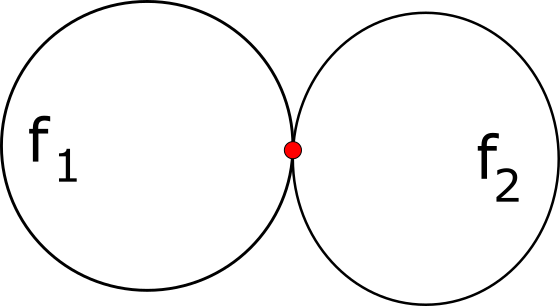
As a simple special case of Example 4 , consider the GIFS depicted in the lower left of Figure 7. It consists of a single vertex and two loop edges $e_{1}$ and $e_{2}$ . Assume that the corresponding functions have scaling ratios

\lambda(f_{1})=s\qquad\lambda(f_{2})=s^{2}

for some $0<s<1$ , so that $d(e_{1})=1,\,d(e_{2})=2$ . Let the parameter be ${\overleftarrow{\theta}}=\overleftarrow{e_{1}}\,\overleftarrow{e_{2}}\,\cdots$ . Then ${\overleftarrow{\theta}}|2=\overleftarrow{e_{1}}\,\overleftarrow{e_{2}}$ and $d(\overleftarrow{\theta}|2)=3$ . The condition on $\sigma$ in the definition of $S_{2}$ in Equation 3.2 is $3<d(\sigma)\leq 3+d(\sigma_{*})$ . The tree $H(S_{2})$ corresponding to the pre-tree $S_{2}$ at the third vertex $e_{2}^{-}$ of $\theta$ , as defined by Proposition 1, is shown at the right in Figure 7. The labels on each edge $e$ is the values $d(e)$ ; the label on each leaf $u$ is the value $d(\sigma)$ of the path $\sigma\in S_{2}$ corresponding to the path in $H(S_{2})$ from the root to $u$ . We will return to this example in Example 8 in Section 4.3, where the red and black colors on the leaves will be explained.

4. GIFS Tilings

For this paper, a tile is a compact subset of ${\mathbb{R}}^{d}$ with nonempty interior, and a tiling of a set $X\subseteq{\mathbb{R}}^{d}$ is a set of pairwise non-overlapping tiles whose union is $X$ .

4.1. The Parameter Space

Let $(G,F)$ be a GIFS. Any path $\overleftarrow{\theta}\in\overleftarrow{\Sigma}^{\infty}$ will be referred to as a parameter of $G$ . Define a metric $d$ on the set $\overleftarrow{\Sigma}^{\infty}$ of parameters by

d(\sigma,\omega)=\begin{cases}0\quad\text{if}\;\sigma=\omega\\ 2^{-k}\quad\text{otherwise, where}\;k\;\text{is the first integer such that}\;\sigma_{k}\neq\omega_{k}\end{cases}.

This makes $(\Sigma,d)$ a compact metric space, which we call the parameter space of the GIFS.

4.2. $\theta$ -tilings

There are infinitely many parameters for a given GIFS, and, for every parameter of the GIFS and every corresponding $\overleftarrow{\theta}$ -sequence ${\mathcal{S}}=\{S_{0},S_{1},S_{2},\dots\}$ , a tiling $T(\overleftarrow{\theta},\mathcal{S})$ will be constructed as follows. For $\sigma\in S_{k}$ :

(4.1)	$\displaystyle t(\overleftarrow{\theta},\mathcal{S},k,\sigma)$	$\displaystyle=f_{\overleftarrow{\theta}\|k}\circ f_{\sigma}(A_{\sigma^{+}})$
	$\displaystyle T(\overleftarrow{\theta},\mathcal{S},k)$	$\displaystyle=\{t(\overleftarrow{\theta},\mathcal{S},k,\sigma)\,:\,\sigma\in S_{k}\}$
	$\displaystyle T(\overleftarrow{\theta},\mathcal{S})$	$\displaystyle=\bigcup_{k=0}^{\infty}T(\overleftarrow{\theta},\mathcal{S},k).$

Note that, in the first line of Equation (4.1), the map $f_{\sigma}$ is a contraction, being the composition of contractions, and $f_{\overleftarrow{\theta}|k}$ is an expansion, being the composition of inverses of contractions. For each $\sigma\in S_{k}$ , the set $t(\overleftarrow{\theta},\mathcal{S},k,\sigma)$ is a single tile. For each $k$ , the set $T(\overleftarrow{\theta},\mathcal{S},k)$ is a patch of tiles. These patches are nested, i.e., $T(\overleftarrow{\theta},\mathcal{S},k)\subset T(\overleftarrow{\theta},\mathcal{S},k+1)$ for all $k$ because, for $\sigma\in S_{k}$ , we have

f_{\overleftarrow{\theta}|k}\circ f_{\sigma}(A_{\sigma^{+}})=f_{\overleftarrow{\theta}|k+1}\circ f_{\theta_{k+1}}f_{\sigma}(A_{\sigma^{+}})=f_{\overleftarrow{\theta}|k+1}\circ f_{\omega}(A_{\omega^{+}}),

where $\omega=f_{\theta_{k+1}}f_{\sigma}\in S_{k+1}$ by condition (2) in the definition of $\overleftarrow{\theta}$ -sequence. The tiling $T(\overleftarrow{\theta},\mathcal{S})$ is the nested union of the patches $T(\overleftarrow{\theta},\mathcal{S},k)$ .

The tiles in a patch $T(\overleftarrow{\theta},\mathcal{S},k)$ are in bijection with the leaves of the tree $H(S_{k})$ as defined in Proposition 1. Specifically, $T(\overleftarrow{\theta},\mathcal{S},k)=\{f_{\overleftarrow{\theta}|k}\circ f_{\sigma}(A_{\sigma^{+}})\,:\,\sigma\in P\}$ , where $P$ is the set of paths in $H(S_{k})$ from the root to a leaf.

Definition 6.

Given a tiling parameter $\overleftarrow{\theta}\in\overleftarrow{\Sigma}^{\infty}$ of a GIFS and a $\overleftarrow{\theta}$ -sequence $\mathcal{S}$ , the tiling $T(\overleftarrow{\theta},\mathcal{S})$ will be called the $(\overleftarrow{\theta},\mathcal{S})$ -tiling or, if $\mathcal{S}$ is understood, then simply the $\overleftarrow{\theta}$ -tiling.

For the set $T(\overleftarrow{\theta},\mathcal{S})$ of tiles, denote by $\langle T(\overleftarrow{\theta},\mathcal{S})\rangle$ the union of these tiles. Call $\overleftarrow{\theta}$ filling if $\langle T(\overleftarrow{\theta},\mathcal{S})\rangle={\mathbb{R}}^{d}$ for all $\overleftarrow{\theta}$ -sequences $\mathcal{S}$ . Theorem 2 states that almost all parameters are filling. A proof is omitted since it is similar to that of [5, Theorems 3.7 and 3.9]. Theorem 3 states that if ${\overleftarrow{\theta}}$ is filling, then $T(\overleftarrow{\theta},\mathcal{S})$ is indeed a tiling of ${\mathbb{R}}^{d}$ .

Theorem 2.

For a GIFS $(G,F)$ , almost all $\overleftarrow{\theta}\in\overleftarrow{\Sigma}^{\infty}$ are filling in the following sense of “almost all”:

(1)

The set of filling $\overleftarrow{\theta}\in\overleftarrow{\Sigma}^{\infty}$ is dense in the parameter space $\overleftarrow{\Sigma}^{\infty}$ .
(2)

Suppose that a positive probability is assigned to each edge such that the sum of the probabilities of the out-edges at each vertex is one, and suppose that a parameter in $\overleftarrow{\Sigma}^{\infty}$ is chosen at random according to these probabilities. Then, with probability 1, this random parameter is filling.

Lemma 1.

For any GIFS and any pre-tree $S$ , the set

W(S):=\{f_{\sigma}(A_{\sigma^{+}}):\sigma\in S\}

is a tiling of the attractor component $A_{r}$ , where $r$ is the root of the pre-tree $S$ .

Proof.

The proof is by induction on the number of paths $|S|$ in the pre-tree $S$ . For $|S|=1$ , the pre-tree consists of a single vertex, and the set $W$ consists of the single tile $A_{r}$ . For $|S|\geq 1$ , assume the assertion is true for all pre-trees with fewer paths. Prune $S$ as follows to obtain a smaller pre-tree $S^{\prime}$ . Let $\sigma=\sigma_{1}\,\sigma_{2}\cdots\sigma_{m}$ be a longest path in $S$ ; let $\sigma^{\prime}:=\sigma_{1}\,\sigma_{2}\cdots\sigma_{m-1}$ ; and let $x$ be the last vertex on $\sigma^{\prime}$ . Then $S^{\prime\prime}:=\{\sigma^{\prime}e\,:\,e\in E_{x}\}$ is a subset of $S$ . Since the set of paths $S^{\prime}:=S\setminus S^{\prime\prime}\cup\{\sigma^{\prime}\}$ is a pre-tree, by the induction hypothesis, $W(S^{\prime})$ is a tiling of $A_{r}$ . Now

	$\displaystyle W(S)$	$\displaystyle=\{f_{\sigma}(A_{\sigma^{+}}):\sigma\in S\setminus S^{\prime\prime}\}\cup\{f_{\sigma}(f_{e}(A_{e^{+}}))\,:\,e\in E_{x}\}$
	$\displaystyle W(S^{\prime})$	$\displaystyle=\{f_{\sigma}(A_{\sigma^{+}}):\sigma\in S\setminus S^{\prime\prime}\}\cup\{f_{\sigma^{\prime}}(A_{x})\}.$

But by Equation (2.4), the set $\{f_{e}(A_{e^{+}})\,:\,e\in E_{x}\}$ is a tiling of $A_{x}$ . Therefore $W(S)$ is a also tiling of $A_{r}$ . ∎

Theorem 3.

Given a GIFS and a parameter $\overleftarrow{\theta}\in\overleftarrow{\Sigma}^{\infty}$ , if $\overleftarrow{\theta}$ is filling, then $T(\overleftarrow{\theta},\mathcal{S})$ is a tiling of ${\mathbb{R}}^{d}$ for every $\overleftarrow{\theta}$ -sequence $\mathcal{S}=\{S_{0},S_{1},\dots\}$ .

Proof.

Since $\overleftarrow{\theta}$ and $\mathcal{S}$ are fixed throughout the proof, we omit them in the notation: let $T(k):=T(\overleftarrow{\theta},\mathcal{S},k),\,T:=T(\overleftarrow{\theta},\mathcal{S})$ . Because it is assumed that $\overleftarrow{\theta}$ is filling, $\langle T\rangle={\mathbb{R}}^{d}$ . Hence, to show that $T$ is a tiling of ${\mathbb{R}}^{d}$ it suffices to show that pairs of distinct tiles in $T$ do not overlap. This is equivalent to showing that, for all $k$ , all pairs of distinct tiles in $T(k)$ do not overlap. By definition, the set of tiles

T(k)=f_{\overleftarrow{\theta}|k}\{f_{\sigma}(A_{\sigma^{+}}):\sigma\in S_{k}\}=f_{\overleftarrow{\theta}|k}W(S_{k}).

By Lemma 1, distinct tiles in $W(S_{k})$ do not overlap. Since the map $f_{\overleftarrow{\theta}|k}$ is a homeomorphism, distinct tiles in $T(k)$ also do not overlap. ∎

4.3. $\theta$ -Tiling Examples

The examples in this section correspond to the four examples of ${\overleftarrow{\theta}}$ -sequences in Section 3.2.

Example 6 (Tilings by Squares).

Consider the GIFS in ${\mathbb{R}}^{2}$ where the graph $G$ consists of a single vertex and four loops, which will be referred to as edges $1,2,3,4$ , and corresponding functions assigned to these loops:

\begin{aligned} f_{1}(x)&=\frac{1}{2}x\\ f_{2}(x)&=\frac{1}{2}x+\Big(\frac{1}{2},0\Big)\end{aligned}\qquad\qquad\begin{aligned} f_{3}(x)&=\frac{1}{2}x+\Big(\frac{1}{2},\frac{1}{2}\Big)\\ f_{4}(x)&=\frac{1}{2}x+\Big(0,\frac{1}{2}\Big).\end{aligned}

The attractor has only one component, which is a square.

If, for a given parameter $\theta$ , the corresponding ${\overleftarrow{\theta}}$ -sequence $\mathcal{S}(\theta)$ is the one given in Example 1 of Section 3.2, then the $(\theta,\mathcal{S}(\theta))$ -tiling is the standard tiling of the plane by unit squares, independent of $\theta$ .

If, on the other hand, the corresponding ${\overleftarrow{\theta}}$ -sequence $\mathcal{S}(\theta,m)$ is the one given in Example 2 of Section 3.2, then taking, for example, $\overleftarrow{\theta}=\overleftarrow{1}\,\overleftarrow{2}\,\overleftarrow{3}\,\overleftarrow{4}\,\overleftarrow{1}\,\overleftarrow{2}\,\overleftarrow{3}\,\overleftarrow{4}\cdots$ and $m=1$ , a patch of the spiral-like $(\theta,\mathcal{S}(\theta,1))$ -tiling is shown in Figure 8. Progressing outward, the squares increase in size.

Example 7 (Uniform Tilings).

Call a tiling uniform if there are positive real numbers $r,R$ such that each tile contains a ball of radius $r$ and is contained in a ball of radius $R$ . Given a parameter $\overleftarrow{\theta}\in{\overleftarrow{\Sigma}}^{\infty}$ for a similarity GIFS, and taking the corresponding ${\overleftarrow{\theta}}$ -sequence $\mathcal{S}(\theta,q,Q)$ of Example 3 of Section 3.2, it is routine to verify that $T(\overleftarrow{\theta},\mathcal{S}(q,Q))$ is a uniform tiling. The tiling that appears in Figure 9 is uniform. Although not apparent in this finite patch, there are infinitely many tile shapes up to congruence, but finitely many up to similarity.

Example 8 (Balanced Tilings).

Definition 7.

For a given similarity GIFS and filling parameter ${\overleftarrow{\theta}}$ , the tiling $T({\overleftarrow{\theta}}):=T({\overleftarrow{\theta}},\mathcal{S}(\theta))$ , where $\mathcal{S}({\overleftarrow{\theta}})$ is the balanced ${\overleftarrow{\theta}}$ -sequence (as in Definition 5), will be referred to as the balanced GIFS tiling.

The order of a tiling is the number of tiles up to congruence.

Proposition 3.

A balanced GIFS tiling has finite order, which is at most $\max\{d(e):e\in E\}$ .

Proof.

Let $d_{\max}=\max\{d(e):e\in E\}$ . Any tile $t\in T(\overleftarrow{\theta},\mathcal{S})$ is, by definition, congruent to $\lambda\,A$ , where $A$ is a component of the attractor and $\lambda=s^{d({\sigma})-d({\overleftarrow{\theta}|k})}$ , where $\sigma\in S_{k}$ for some $k$ . By the definition of $S_{k}$ as given in Equation (3.2), we have

0<d({\sigma})-d({\overleftarrow{\theta}|k})\leq d_{\max}.

Therefore there are at most finitely many possibilities for $\lambda$ . ∎

A balanced tiling corresponding to the GIFS in Figure 7 in Example 5 is shown in Figure 10. In this case the scaling constant $s$ in Definition 5 is the square root of the golden ratio $(1+\sqrt{5})/2$ . In this tiling there are two similar Ammann tiles, a small one and a large one. In the tree $H(S_{2})$ in Figure 7, the red leaves correspond to the large tiles in the patch $T({\overleftarrow{\theta}},\mathcal{S},2)$ and the black leaves correspond to the small tiles.

In [3] Bandt and Gummelt construct fractal versions of the Penrose kite and dart. A balanced tiling construction of a fractal Penrose tiling is shown in Figure 11. The directed graph consisting of two vertices and five edges (3 loops) is shown on the left. The scaling ratio of each of the five functions (whose formulas are omitted) is the reciprocal of the golden ratio.

The tilings in Figures 12, 13, and 14, as well as those in Figures 4 and 5, are also examples of balanced GIFS tilings.

4.4. Tile Addresses

Assume that the parameter ${\overleftarrow{\theta}}$ of a GIFS is fixed. Each tile in $t\in T(\overleftarrow{\theta},\mathcal{S})$ can be uniquely expressed as $t=f_{\overleftarrow{\theta}|k}\circ f_{\sigma}(A_{\sigma^{+}})$ , where $\theta_{k}^{-}\neq\sigma_{1}$ . Define the unique address of tile $t$ to be $k\bullet\sigma$ . The proposition below follows from the definition of the address and Equation (2.3).

Proposition 4.

If the address of a tile $t\in T(\overleftarrow{\theta},\mathcal{S})$ is $k\bullet\sigma$ , then

t=\Big\{f_{\overleftarrow{\theta}|k}\big(\lim_{j\rightarrow\infty}f_{\sigma\alpha|j}(x_{0})\big)\,:\,\alpha\in\Sigma^{\infty},\,\alpha^{-}=\sigma^{+}\Big\},

where the limit is independent of the point $x_{0}\in{\mathbb{R}}^{d}$ .

5. Tiling Hierarchy

Given a parameter ${\overleftarrow{\theta}}$ of a GIFS and two ${\overleftarrow{\theta}}$ -sequences ${\mathcal{S}}=\{S_{0},S_{1},S_{2},\dots\}$ and ${\mathcal{S}^{\prime}}=\{S^{\prime}_{0},S^{\prime}_{1},S^{\prime}_{2},\dots\}$ such that $\mathcal{S}\neq\mathcal{S}^{\prime}$ , we say that ${\mathcal{S}^{\prime}}$ lies above $\mathcal{S}$ if, for every $k$ , each path in $S^{\prime}_{k}$ is a subpath of a path in $S_{k}$ .

Lemma 2.

If ${\mathcal{S}^{\prime}}$ lies above $\mathcal{S}$ , then each tile in $T({\overleftarrow{\theta}},\mathcal{S}^{\prime})$ is tiled by tiles in $T({\overleftarrow{\theta}},\mathcal{S})$ .

Proof.

It is sufficient to show that each $t\in T({\overleftarrow{\theta}},\mathcal{S})$ is contained in a tile $t^{\prime}\in T({\overleftarrow{\theta}},\mathcal{S}^{\prime})$ . Let $t=f_{\overleftarrow{\theta}|k}\circ f_{\sigma}(A_{\sigma^{+}})\in T({\overleftarrow{\theta}},\mathcal{S})$ . Since ${\mathcal{S}^{\prime}}$ lies above $\mathcal{S}$ , there is a path $\omega\in S^{\prime}_{k}$ such that $\omega$ is a subpath of $\sigma$ . We claim that $t\in f_{\overleftarrow{\theta}|k}\circ f_{\omega}(A_{\omega^{+}})\in T({\overleftarrow{\theta}},\mathcal{S}^{\prime})$ , which would complete the proof. The claim, however, follows in same way as the proof of Lemma 1. ∎

Definition 8.

Given a sequence $\mathcal{S}_{0},\mathcal{S}_{1},\mathcal{S}_{2},\dots$ of ${\overleftarrow{\theta}}$ -sequences such that $\mathcal{S}_{k+1}$ lies above $\mathcal{S}_{k}$ for all $k$ , the sequence of tilings

T({\overleftarrow{\theta}},\mathcal{S}_{0}),T({\overleftarrow{\theta}},\mathcal{S}_{1}),T({\overleftarrow{\theta}},\mathcal{S}_{2}),\dots

is called a hierarchy for the tiling $T({\overleftarrow{\theta}}):=T({\overleftarrow{\theta}},\mathcal{S}_{0})$ . The term “hierarchy” is used because, as follows from Lemma 2, each tile in $T({\overleftarrow{\theta}},\mathcal{S}_{k})$ is contained in a tile in $T({\overleftarrow{\theta}},\mathcal{S}_{k+1})$ , for all $k$ .

5.1. Hierarchies for a Balanced GIFS Tiling

For a fixed similarity GIFS, fix a parameter $\overleftarrow{\theta}\in{\overleftarrow{\Sigma}}^{\infty}$ . Let $\mathcal{S}$ denote the balanced ${\overleftarrow{\theta}}$ -sequence as in Definition 5, so that $T({\overleftarrow{\theta}},\mathcal{S})$ is the corresponding balanced GIFS tiling. We now introduce two particular hierarchies in the balanced case.

For integers $n,k\geq 0$ , let

	$\displaystyle S_{(n,k)}$	$\displaystyle=\big\{\sigma\in\Sigma^{}\,:\,\sigma^{-}=\theta_{k}^{-}\quad\text{and}\quad 0<d(\sigma)-d(\overleftarrow{\theta}\|k)+d(\overleftarrow{\theta}\|n)\leq d(\sigma_{})\big\}$
	$\displaystyle\widehat{S}_{(n,k)}$	$\displaystyle=\big\{\sigma\in\Sigma^{}\,:\,\sigma^{-}=\theta_{k}^{-}\quad\text{and}\quad 0<d(\sigma)-d(\overleftarrow{\theta}\|k)+n\leq d(\sigma_{})\big\}$

and

	$\displaystyle{\mathcal{S}}_{n}$	$\displaystyle:=\mathcal{S}_{n}(\overleftarrow{\theta})=(S_{n,0},S_{n,1},S_{n,2},\dots)$
	$\displaystyle{\widehat{\mathcal{S}}}_{n}$	$\displaystyle:=\widehat{\mathcal{S}}_{n}(\overleftarrow{\theta})=(\widehat{S}_{n,0},\widehat{S}_{n,1},\widehat{S}_{n,2},\dots).$

Note that $\mathcal{S}_{0}=\mathcal{S}$ and, for $n\geq 1$ , the first few terms in the above sequences may be empty. As in Proposition 2, it is not hard to show that ${\mathcal{S}}_{n}$ and ${\widehat{\mathcal{S}}}_{n}$ are $\overleftarrow{\theta}$ -sequences. And, according to Proposition 5 below, the corresponding sequences of tilings

\mathcal{T}:=(T_{0},T_{1},T_{2},\dots)\qquad\text{and}\qquad\widehat{\mathcal{T}}:=(\widehat{T}_{0},\widehat{T}_{1},\widehat{T}_{2},\dots),

where $T_{n}=T(\overleftarrow{\theta},\mathcal{S}_{n})$ and $\widehat{T}_{n}=\widehat{T}(\overleftarrow{\theta},\widehat{\mathcal{S}}_{n})$ , are tiling hierarchies. Call these balanced tiling hierarchies. The subscript $n$ is referred to as the level of the tiling in the hierarchy. For the chair tiling shown in Figure 1, the balanced hierarchies $\mathcal{T}$ and $\widehat{\mathcal{T}}$ are the same, the first three levels of the hierarchy shown using thicker lines in Figure 1.

Definition 9.

For a similarity GIFS and for each $i=1,2,\dots,N$ , let $B_{i}:=\{f_{e}(A_{e^{+}}):e\in E_{i}\}$ . These sets are fundamental objects of the GIFS because the $i^{\text{th}}$ component $A_{i}$ of the attractor is, by definition, $A_{i}=\bigcup\{X:X\in B_{i}\}$ . Call any set congruent to $s^{j}\,B_{i}:=\{s^{j}\,f_{e}(A_{e+}):e\in E_{i}\}$ , where $s$ is the scaling constant, a basic $i$ -subdivision. For example, for the tiling in Figure 4, the four basic subdivisions, up to a similarity, are shown in Figure 15.

Basic subdivisions occur as patches in a balanced tiling $T({\overleftarrow{\theta}},\mathcal{S})$ when, in the tree $H(S_{k})$ (as defined in Proposition 1), there is a vertex $i$ all of whose children are leaves. In this case the basic subdivision is $B_{i}=\{t({\overleftarrow{\theta}},\mathcal{S},k,\sigma)\,:\,\sigma\in P_{i}\}$ , where $P_{i}$ is the set of paths in the pre-tree $S_{k}$ corresponding to the paths in $H(S_{k})$ from the root to a child of vertex $i$ . The union of the tiles in $B_{i}$ is a set that is similar to the component $A_{h(i)}$ of the attractor, where $h$ is the homomorphism of Proposition 1.

Proposition 5.

Given a parameter $\overleftarrow{\theta}\in\overleftarrow{\Sigma}^{\infty}$ for a similarity GIFS, the sequences

\mathcal{T}:=(T_{0},T_{1},T_{2},\dots)\qquad\text{and}\qquad\widehat{\mathcal{T}}:=(\widehat{T}_{0},\widehat{T}_{1},\widehat{T}_{2},\dots),

where $T_{n}=T(\overleftarrow{\theta},\mathcal{S}_{n})$ and $\widehat{T}_{n}=\widehat{T}(\overleftarrow{\theta},\widehat{\mathcal{S}}_{n})$ , have the following properties:

(1)

$T_{0}=\widehat{T}_{0}=T({\overleftarrow{\theta}},\mathcal{S})$ ;
(2)

$\mathcal{T}$ and $\widehat{\mathcal{T}}$ are hierarchies for the balanced GIFS tiling $T({\overleftarrow{\theta}},\mathcal{S})$ ;
(3)

$\widehat{\mathcal{T}}$ is a refinement of the hierarchy $\mathcal{T}$ in that every tiling in $\mathcal{T}$ appears in $\widehat{\mathcal{T}}$ ;
(4)

each tile in $\widehat{T}_{n+1}$ is either a tile in $\widehat{T}_{n}$ or the union of tiles in $\widehat{T}_{n}$ that comprise a basic subdivision.

Proof.

Statement (1) follows from the fact that $S_{(0,k)}=\widehat{S}_{(0,k)}$ . Statement (2) follows from Lemma 2. Statement (3) follows directly from the definitions.

Concerning statement (4), if tile $t=t({\overleftarrow{\theta}},\widehat{\mathcal{S}}_{n+1},k,\sigma)\in\widehat{T}_{n+1}$ is not a tile in $\widehat{T}_{n}$ , then $0<d(\sigma)-d(\overleftarrow{\theta}|k)+(n+1)\leq d(\sigma_{*})$ , but $0\geq d(\sigma)-d(\overleftarrow{\theta}|k)+n$ . Therefore $d(\sigma)-d(\overleftarrow{\theta}|k)+n=0$ , which implies that $\sigma\,e\in\widehat{S}_{(n,k)}$ for all $e\in E_{\sigma^{+}}$ . Hence $t({\overleftarrow{\theta}},\widehat{\mathcal{S}}_{n},k,\sigma\,e)\in\widehat{T}_{n}$ for all $e\in E_{\sigma^{+}}$ and

t=\bigcup_{e\in E_{\sigma^{+}}}\,t({\overleftarrow{\theta}},\widehat{\mathcal{S}}_{n},k,\sigma\,e)=f_{{\overleftarrow{\theta}}|k}\circ f_{\sigma}\circ f_{e}(A_{e+}),

which, by definition, is a basic subdivision. ∎

5.2. The Tiling Map

Given a similarity GIFS, denote by $\mathbb{T}$ the set of all balanced GIFS tilings. Define a metric on $\mathbb{T}$ as follows. Let $\rho:{\mathbb{R}}^{d}\rightarrow\mathbb{S}^{d}$ be the usual stereographic projection onto the $d$ -sphere, obtained by positioning $\mathbb{S}^{d}$ at the origin. Let $\mathbb{H}(\mathbb{S}^{d})$ be the set of nonempty closed subsets of $\mathbb{S}^{d}$ and $d_{\mathbb{H}(\mathbb{S}^{d})}$ the corresponding Hausdorff distance with respects to the round metric on $\mathbb{S}^{d}$ . Let $\mathbb{H}(\mathbb{H}(\mathbb{S}^{d}))$ be the collection of nonempty compact subsets of the compact metric space $(\mathbb{H}(\mathbb{S}^{d}),d_{\mathbb{H}(\mathbb{S}^{d})})$ . For tilings $T,T^{\prime}$ define

d^{\prime}(T,T^{\prime})=d_{\mathbb{H}(\mathbb{H}(\mathbb{S}^{d}))}(\rho(T),\rho(T^{\prime})).

Define the map $W:{\mathbb{T}}\rightarrow{\mathbb{T}}$ on the tiling space by

W(T(\overleftarrow{\theta}))=f_{\theta_{1}}(T_{1}(\overleftarrow{\theta})),

where $T_{1}$ is the level $1$ tiling in the hierarchy $\mathcal{T}$ . In other words, $W(T(\overleftarrow{\theta}))$ is, up to the similarity transformation $f_{\theta_{1}}$ , the tiling at level $1$ in the hierarchy of the tiling $T(\overleftarrow{\theta},\mathcal{S})$ .

For any $\overleftarrow{\theta}=\overleftarrow{\theta}_{1}\,\overleftarrow{\theta}_{2}\,\overleftarrow{\theta}_{3}\cdots\in\overleftarrow{\Sigma}^{\infty}$ , define the shift map $w:\overleftarrow{\Sigma}^{\infty}\rightarrow\overleftarrow{\Sigma}^{\infty}$ on the parameter space by $w(\overleftarrow{\theta})=\overleftarrow{\theta}_{2}\,\overleftarrow{\theta}_{3}\cdots$ .

Call the map $T:\overleftarrow{\Sigma}^{\infty}\rightarrow\mathbb{T}$ from the parameter space to the tiling space that takes $\overleftarrow{\theta}$ to $T(\overleftarrow{\theta})$ the tiling map. The theorem below states that, via the tiling map, the shift map on the paramater space corresponds to the map $W$ on the tiling space.

Theorem 4.

The tiling map $T$ is continuous and the following diagram commutes.

\begin{array}[c]{ccccc}&&w&&\\ &\overleftarrow{\Sigma}^{\infty}&\rightarrow&\overleftarrow{\Sigma}^{\infty}&\\ T&\Big\downarrow&&\Big\downarrow&T\\ &{\mathbb{T}}&\rightarrow&{\mathbb{T}}&\\ &&W&&\end{array}

Proof.

Given an positive real number $R$ and two parameters ${\overleftarrow{\theta}}$ and $\overleftarrow{\theta^{\prime}}$ , there is a $k$ such that both patches $T({\overleftarrow{\theta}},k)$ and $T(\overleftarrow{\theta^{\prime}},k)$ contain the ball of radius $R$ centered at the origin. If ${\overleftarrow{\theta}}|k=\overleftarrow{\theta^{\prime}}|k$ , i.e., if ${\overleftarrow{\theta}}$ and $\overleftarrow{\theta^{\prime}}$ are sufficiently close in the parameter space metric, then $T({\overleftarrow{\theta}},k)=T(\overleftarrow{\theta^{\prime}},k)$ , which guarantees that the $T({\overleftarrow{\theta}})$ and $T(\overleftarrow{\theta^{\prime}})$ are close in the tiling space metric.

Concerning the commuting diagram we have

	$\displaystyle{f_{\theta_{1}}}^{-1}(T(w(\overleftarrow{\theta}))$	$\displaystyle=\Big\{f_{\overleftarrow{\theta}\|k}\circ f_{\sigma}:\sigma=\sigma_{1}\cdots\sigma_{j},\;0<d(\sigma)-d(\theta\|k)+d(\theta_{1})\leq d(\sigma_{j})\Big\}$
		$\displaystyle=T_{1}(\overleftarrow{\theta}).$

Therefore $T(w(\overleftarrow{\theta}))=W(T(\overleftarrow{\theta}))$ . ∎

6. Properties of Balanced Tilings

6.1. When is a balanced tiling self-similar?

Definition 10.

For a closed path $\alpha$ in a directed graph, let $\overline{\alpha}:=\alpha\alpha\cdots$ . A path $\theta\in\Sigma^{\infty}$ is periodic if there is an $\alpha\in\Sigma^{*}$ such that $\theta=\overline{\alpha}$ and eventually periodic if there are $\alpha,\beta\in\Sigma^{*}$ such that $\theta=\beta\overline{\alpha}$ .

Theorem 5.

If $\overleftarrow{\theta}\in\overleftarrow{\Sigma}^{\infty}$ is eventually periodic, then the balanced GIFS tiling $T(\overleftarrow{\theta})$ is self-similar.

Proof.

Let ${\overleftarrow{\theta}}=\beta\,\overline{\alpha}$ , where $\alpha,\beta\in\overleftarrow{\Sigma}^{*}$ . We may assume, without loss of generality, that $k$ is sufficiently large so that ${\overleftarrow{\theta}}|k=\beta\,\alpha^{q}\,\gamma$ for some $q\in\mathbb{N}$ and some $\gamma\in\overleftarrow{\Sigma}^{*}$ . Since $\alpha$ is a closed path, the end vertex of $\beta\,\alpha^{q}\,\gamma$ is independent of the integer $q$ . Let $t=f_{{\overleftarrow{\theta}}|k}\circ f_{\sigma}(A_{\sigma^{+}})\in T({\overleftarrow{\theta}})$ , where $0<d(\sigma)-d(\beta\,\alpha^{q}\,\gamma)\leq d(\sigma_{*}).$ It is sufficient to find a similarity transformation $\phi$ such that $\phi(t)$ is tiled by tiles in $T({\overleftarrow{\theta}})$ .

As in the proof of Proposition 2, the set of paths

S=\{\omega\in\Sigma\,:\,\omega^{-}=\sigma^{+}\;\text{and}\;0<d(\omega)-d(\alpha)+d(\sigma)-d(\beta\,\alpha^{q}\,\gamma)\leq d(\omega_{*})\}

is a pre-tree. Therefore, by Lemma 1,

A_{\sigma^{+}}=\bigcup\Big\{f_{\omega}(A_{\omega^{+}}):0<d(\sigma\omega)-d(\beta\alpha^{q+1}\gamma)\leq d(\omega_{*})\Big\}.

Let $\phi=f_{\beta}\circ f_{\alpha^{m}}\circ{f_{\beta}}^{-1}$ , where $m$ is the least positive integer such that $d(\beta\alpha^{m}\gamma)\geq d(\sigma)$ . Then $S\neq\emptyset$ , and we have

	$\displaystyle\phi(t)$	$\displaystyle=f_{\beta}\circ f_{\alpha}\circ{f_{\beta}}^{-1}\circ f_{{\overleftarrow{\theta}}\|k}\circ f_{\sigma}(A_{\sigma^{+}})=f_{\beta}\circ(f_{\alpha})^{q+1}\circ f_{\gamma}\circ f_{\sigma}(A_{\sigma^{+}})$
		$\displaystyle=\bigcup\Big\{(f_{\beta}\circ(f_{\alpha})^{q+1}\circ f_{\gamma})\circ f_{\sigma}\circ f_{\omega}(A_{\omega^{+}}):0<d(\sigma\omega)-d(\beta\alpha^{q+1}\gamma)\leq d(\omega_{*})\Big\}$
		$\displaystyle=\bigcup\Big\{(f_{\beta}\circ(f_{\alpha})^{q+1}\circ f_{\gamma})\circ f_{\sigma\omega}(A_{(\sigma\omega)^{+}}):0<d(\sigma\omega)-d(\beta\alpha^{q+1}\gamma)\leq d((\sigma\omega)_{*})\Big\}.$

But, by definition, the sets in the above union are tiles in $T({\overleftarrow{\theta}})$ . ∎

6.2. When is a balanced tiling repetitive?

Definition 11.

Let $(G,F)$ be a GIFS with directed graph $G=(V,E)$ . We say that $(G,F)$ satisfies the triangle property if there exists an integer $N$ such that, for all $u,v,w\in V$ , if $\sigma(u,v)$ is a path from $u$ to $v$ and $\sigma(u,w)$ is a path from $u$ to $w$ such that $d(\sigma(u,v))-d(\sigma(u,w))\geq N$ , then there is a path $\sigma(w,v)$ from $w$ to $v$ such that

d(\sigma(u,v))=d(\sigma(u,w))+d(\sigma(w,v)).

We say that $(G,F)$ is coprime if there is a vertex $x$ in $G$ and closed paths $\omega_{1},\omega_{2},\cdots,\omega_{m},\,m\geq 2,$ containing $x$ such that $\gcd\,(d(\omega_{1}),d(\omega_{2}),\cdots,d(\omega_{m}))=1$ .

Lemma 3.

If $(G,F)$ is coprime, then $(G,F)$ satisfies the triangle property.

Proof.

Assume $(G,F)$ is coprime. By a standard number theoretic result, there is an integer $N_{1}$ such that every integer greater than or equal to $N_{1}$ can be expressed as $\sum_{i=1}^{m}a_{i}d(\omega_{i})$ for some non-negative integers $a_{i}$ . Since $G$ is strongly connected, every two vertices are connected by a finite path. Let $N_{2}$ be an integer such that every two vertices are joined by a path whose $d$ -value is at most $N_{2}$ . To show that $(G,F)$ satisfies the triangle property, consider any three vertices $u,v,w\in V$ , and let $N=N_{1}+2N_{2}$ . Assume that $N_{0}:=d(\sigma(u,v))-d(\sigma(u,w))\geq N$ . The path $\sigma(w,v)$ required in the definition of the triangle property is obtained as follows. If $x$ is the vertex in the definition of coprime GIFS, let $\sigma(w,v)$ be a path from $w$ to $v$ that is the concatenation of the three paths $\sigma(w,x)$ , $\sigma(x,x)$ , and $\sigma(x,v)$ , where $\sigma(w,x)$ and $\sigma(x,v)$ are any paths from $w$ to $x$ and from $x$ to $v$ , respectively, such that $q_{1}:=d(\sigma(w,x))\leq N_{2},\,q_{2}:=d(\sigma(x,v))\leq N_{2}$ . Let $\sigma(x,x)$ be obtained by, starting and ending at $x$ , traversing the closed paths $\omega_{1},\omega_{2},\cdots,\omega_{m}$ (as defined in the definition of coprime) sufficiently many time so that $d(\sigma(x,x))=N-q_{1}-q_{2}$ . This is possible because $N-q_{1}-q_{2}\geq N-2N_{2}\geq N_{1}$ . Now $d(w,v)=q_{1}+(N-q_{1}-q_{2})+q_{2}=N$ . ∎

Remark 1.

If the digraph has just one vertex (the IFS case), then the GIFS is coprime if and only if $g:=\gcd\{d(e),e\in E\}=1$ , which can always, without loss of generality, be assumed by replacing the scaling constant $s$ by $s^{g}$ .

Theorem 6.

If a similarity GIFS satisfies the triangle property, then the balanced tiling $T(\overleftarrow{\theta})$ is repetitive for all parameters $\theta$ .

Proof.

Since, by definition, $\theta$ is assumed filling for a balanced GIFS tiling, any patch of $T(\overleftarrow{\theta})$ is contained in $T(\overleftarrow{\theta},k)$ for some $k$ . It then suffices to show that there exists an integer $n$ such that a copy congruent to $T(\overleftarrow{\theta},k)$ is contained in every tile of $T_{n}$ in the $n^{th}$ -level of the hierarchy $\mathcal{T}$ defined in Section 5. Let $v=\theta_{k}^{-}$ , i.e., the last vertex of $\overleftarrow{\theta}|k$ . Choose $K>k$ and choose level $n$ such that the following holds for every $t=f_{\overleftarrow{\theta}|K}\circ f_{\sigma}(A_{\sigma^{+}})\in T_{n}$ : if $u=\theta_{K}^{-},\;x=\sigma^{+}$ , and $\sigma(u,v)=\theta_{K}\theta_{K-1}\cdots\theta_{k+1}$ , then $d(\sigma(u,v))-d(\sigma)\geq N$ , where $N$ is as in Definition 11. By the triangle property, there is a path $\sigma(x,v)$ from $x$ to $v$ such that $d(\sigma(u,v))=d(\sigma(u,x))+d(\sigma(x,v)).$ Now

T({\overleftarrow{\theta}},k)=\{f_{{\overleftarrow{\theta}}|k}\circ f_{\omega}(A_{\omega^{+}})\,:\,\omega^{-}=u,\;0<d(\omega)-d({\overleftarrow{\theta}}|k)\leq d(\omega_{*})\}.

T=\{f_{{\overleftarrow{\theta}}|K}\circ f_{\sigma(u,x)\sigma(x,v)\omega}(A_{\omega^{+}})\,:\,\omega^{-}=u,\;0<d(\omega)-d({\overleftarrow{\theta}}|k)\leq d(\omega_{*})\},

then $T({\overleftarrow{\theta}},k)$ and $T$ are isometric because

	$\displaystyle d({\overleftarrow{\theta}}\|k\,\omega)$	$\displaystyle=-d({\overleftarrow{\theta}}\|k)+d(\omega)$
		$\displaystyle=-d({\overleftarrow{\theta}}\|k)-d(\sigma(u,v))+d(\sigma(u,x))+d(\sigma(x,v))+d(\omega)$
		$\displaystyle=-d({\overleftarrow{\theta}}\|K)+d(\sigma(u,x)\sigma(x,v)\omega).$

But each tile in $T$ is contained in $t\in T_{n}$ because $f_{\sigma(x,v)\omega}(A_{\omega^{+}})\subset A_{\sigma^{+}}$ implies that $f_{{\overleftarrow{\theta}}|K}\circ f_{\sigma(u,x)}\circ f_{\sigma(x,v)\omega}(A_{\omega^{+}})\subset f_{{\overleftarrow{\theta}}|K}\circ f_{\sigma}(A_{\sigma^{+}})$ . ∎

The following corollary follows immediately from Theorem 6 and Lemma 3.

Corollary 1.

If a similarity GIFS is coprime, then the balanced tiling $T(\overleftarrow{\theta})$ is repetitive for all parameters $\theta$ .

6.3. When is a balanced tiling non-periodic?

Definition 12.

For a basic subdivison $B$ , let $\cup B$ denote the union of the tiles in $B$ . A similarity GIFS is called rigid if the following property holds for any basic $i$ -subdivision $B$ and any $i^{\prime}$ -subdivision $B^{\prime}$ : if the intersection $B\cap B^{\prime}$ is a nonempty set that tiles $(\cup B)\cap(\cup B^{\prime})$ , then $i=i^{\prime}$ and $B=B^{\prime}$ .

In Example 6 of Section 4.3, there is a basic subdivision $B$ into four unit squares. Clearly two congruent copies (red and blue) of $B$ can intersect in a single square as in Figure 16, implying that the GIFS of Example 6 is not rigid.

The following lemma states that, for a given rigid similarity GIFS, a tile preserving isometry taking one balanced tiling onto another preserves the hierarchical structure.

Lemma 4.

If $(G,F)$ is rigid and if $\Phi$ is an isometry of ${\mathbb{R}}^{d}$ that maps $T(\overleftarrow{\theta})$ to $T(\overleftarrow{\theta^{\prime}})$ , then $\Phi$ maps tiles in $\cup_{n=1}^{\infty}\widehat{T}_{n}(\overleftarrow{\theta})$ to tiles in $\cup_{n=1}^{\infty}\widehat{T}_{n}(\overleftarrow{\theta^{\prime}})$ .

Proof.

It will be proved by induction on the level $n$ , that every tile in $\widehat{T}_{n}(\overleftarrow{\theta})$ is mapped by $\Phi$ to a tile in $\cup_{k=1}^{\infty}\widehat{T}_{k}(\overleftarrow{\theta^{\prime}})$ . By the hypothesis, this is true for $n=0$ ; assume that it is true for all $m<n$ . Assume, by way of contradiction, that a tile $t\in\widehat{T}_{n}(\overleftarrow{\theta})$ is not mapped to a tile in $\cup_{k=1}^{\infty}\widehat{T}_{k}(\overleftarrow{\theta^{\prime}})$ . Let $m$ be the largest level less than $n$ such that $t$ is tiled by a set $Q$ of at least $2$ tiles in $\widehat{T}_{m}(\overleftarrow{\theta})$ . By the induction hypothesis, the image under $\Phi$ of each tile in $Q$ is a tile in $\cup_{k=1}^{\infty}\widehat{T}_{k}(\overleftarrow{\theta^{\prime}})$ . For each tile $q\in Q$ , let $M_{q}$ be the least integer for which there exists a $t^{\prime}_{q}\in\widehat{T}_{M_{q}}(\overleftarrow{\theta^{\prime}})$ such that $\Phi(q)\subsetneq t^{\prime}_{q}$ . There is some $q_{0}\in Q$ such that no $q\in Q$ exists such that $t^{\prime}_{q}\subsetneq t^{\prime}:=t^{\prime}_{q_{0}}$ . Let $m^{\prime}$ be the largest integer less then $M_{q_{0}}$ such that $t^{\prime}_{q_{0}}\notin\widehat{T}_{m^{\prime}}$ . Let $Q^{\prime}$ denote the set of tiles of $T_{m^{\prime}}$ that tile $t^{\prime}$ . Then $\Phi(t)\cap t^{\prime}$ is tiled by $\Phi(Q)\cap Q^{\prime}$ . But $Q$ is a basic subdivision of $t$ and $Q^{\prime}$ is a basic subdivision of $t^{\prime}$ . Then $\Phi(t)\neq t^{\prime}$ contradicts the rigidity assumption. ∎

Theorem 7.

If a similarity GIFS is rigid, then, for all ${\overleftarrow{\theta}}$ , the balanced tiling $T(\overleftarrow{\theta})$ is not periodic.

Proof.

Assume, by way of contradiction, that $T=T(\overleftarrow{\theta})$ is periodic. Then it has a translation symmetry $\tau$ . By Lemma 4, the translation $\tau$ maps, for all $n$ , tiles in $\widehat{T}_{n}$ to tiles in $\bigcup_{n=0}^{\infty}\widehat{T}_{n}$ . This leads to a contradiction since the size of the tiles in $\widehat{T}_{n}$ eventually dwarfs the translational distance of $\tau$ . ∎

6.4. When are two balanced tilings congruent?

Two tilings are said to be congruent if there is a tile preserving isometry taking one tiling to the other.

Lemma 5.

If balanced tilings $T({\overleftarrow{\theta}})$ and $T(\overleftarrow{\theta^{\prime}})$ for a rigid GIFS are congruent, then there exist integers $K$ and $K^{\prime}$ such that $w^{K}({\overleftarrow{\theta}})=w^{K^{\prime}}(\overleftarrow{\theta^{\prime}})$ , where $w$ is the shift map on parameter space.

Proof.

Given a rigid GIFS $(G,F)$ and a parameter $\theta\in\overleftarrow{\Sigma}^{\infty}$ , let $t_{0}\in T({\overleftarrow{\theta}})=\widehat{T}_{0}$ . Define a sequence of tiles

t_{0}\subsetneq t_{1}\subsetneq t_{2}\subsetneq t_{3}\subsetneq\cdots

inductively as follows: $t_{n+1}$ is the minimal (with respect to containment) tile properly containing $t_{n}$ that belongs to a tiling in the hierarchy $\widehat{T}_{0}({\overleftarrow{\theta}}),\widehat{T}_{1}({\overleftarrow{\theta}}),\widehat{T}_{2}({\overleftarrow{\theta}}),\dots$ . For a given $k$ , if $t_{0}=t(\theta,\mathcal{S},k,\sigma)=f_{\overleftarrow{\theta}|k}\circ f_{\sigma}(A_{\sigma^{+}})$ , let the vertices of $\sigma$ be $v_{0},v_{1},v_{2},\dots,v_{m}$ , going from the end of $\sigma$ to its beginning (the root of the pre-tree). Then

(6.1)

t_{j}=f_{\overleftarrow{\theta}|k}\circ f_{\sigma|m-j}(A_{v_{j}})

for $0\leq j\leq m$ .

Now assume that there is an isometry $\Phi$ that takes tiling $T({\overleftarrow{\theta}})$ to $T(\overleftarrow{\theta}^{\prime})$ . Let $t_{0}\in T({\overleftarrow{\theta}})$ and $t_{0}^{\prime}=\Phi(t_{0})\in T(\overleftarrow{\theta}^{\prime})$ . Let

t_{0}\subsetneq t_{1}\subsetneq t_{2}\subsetneq t_{3}\cdots\qquad\text{and}\qquad t^{\prime}_{0}\subsetneq t^{\prime}_{1}\subsetneq t^{\prime}_{2}\subsetneq t^{\prime}_{3}\cdots

be the respective hierarchical sequences of tiles defined in the previous paragraph. With notation as above, the formula corresponding to Equation (6.1) is, with sufficiently large $k$ ,

(6.2)

t_{j}^{\prime}=f_{\overleftarrow{\theta^{\prime}}|k}\circ f_{\sigma^{\prime}|m^{\prime}-j}(A_{v^{\prime}_{j}})

for $0\leq j\leq m^{\prime}$ .

We now prove by induction that $t^{\prime}_{n}=\Phi(t_{n})$ for all $n\geq 0$ . It is true by assumption for $n=0$ . Assume that $t^{\prime}_{n}=\Phi(t_{n})$ . By Lemma 4, $\Phi(t_{n+1})$ is a tile in $\bigcup_{n=1}^{\infty}\widehat{T}_{n}$ . If $\Phi(t_{n+1})=t_{n+1}^{\prime}$ , then we are done; otherwise there is a tile $t^{\prime}\in\bigcup_{n=1}^{\infty}\widehat{T}_{n}$ such that $t_{n}^{\prime}\subsetneq t^{\prime}\subsetneq\Phi(t_{n+1})$ . But, again by Lemma 4, $\Phi^{-1}(t^{\prime})$ is a tile in $\bigcup_{n=1}^{\infty}\widehat{T}_{n}$ such that $t_{n}\subsetneq\Phi^{-1}\subsetneq t_{n+1}$ , which contradicts the definition of $t_{n+1}$ as the minimal tile properly containing $t_{n}$ .

Since the basic subdivision of $t_{n}$ is the same as the basic subdivision of $t_{n}^{\prime}$ for all $n\geq 1$ , by rigidity we have $v_{0}^{\prime}=v_{0},v_{1}^{\prime}=v_{1},v_{2}^{\prime}=v_{2},\dots$ . Assuming, without loss of generality, that path $\sigma$ is at least as long as $\sigma^{\prime}$ , this implies that the part of $\sigma^{\prime}$ between the vertex $v^{\prime}_{m^{\prime}}$ to vertex $v^{\prime}_{0}$ (the whole path $\sigma^{\prime}$ ) is the same path as the part of $\sigma$ from vertex $v_{m^{\prime}}$ to vertex $v_{0}$ .

Now take $M$ sufficiently large so that the following holds. Expressing $t_{0}=f_{\overleftarrow{\theta}|M}\circ f_{\widehat{\sigma}}(A_{\widehat{\sigma}^{+}})$ , it must be the case that $\widehat{\sigma}=\theta_{M}\,\theta_{M-1}\cdots\theta_{k+1}\sigma$ . Similarly $\widehat{\sigma}^{\prime}=\theta_{M}\,\theta_{M-1}\cdots\theta_{k+1}\sigma^{\prime}$ . But by the last sentence of the previous paragraph this implies that

-\theta_{k+1}\,-\theta_{k+2}\cdots-\theta_{M-(m-m^{\prime})}=-\theta^{\prime}_{k+1+(m-m^{\prime})}\,-\theta_{k+2+(m-m^{\prime})}\cdots-\theta^{\prime}_{M}.

Since $M$ can be arbitrarily large, applying the shift operator yields

w^{k}({\overleftarrow{\theta}})=w^{k+(m-m^{\prime})}(\overleftarrow{\theta^{\prime}}).

∎

Definition 13.

For a given GIFS, call two parameters ${\overleftarrow{\theta}},\overleftarrow{\theta^{\prime}}$ equivalent if there exist integers $K,K^{\prime}$ such that $d({\overleftarrow{\theta}}|K)=d(\overleftarrow{\theta^{\prime}}|K^{\prime})$ and $w^{K}({\overleftarrow{\theta}})=w^{K^{\prime}}(\overleftarrow{\theta^{\prime}})$ , where $w$ is the shift map. In other words, beginning segments of ${\overleftarrow{\theta}}$ have the same $d$ -value, and the tails are identical.

Theorem 8.

For a given GIFS and parameters ${\overleftarrow{\theta}}$ and $\overleftarrow{\theta^{\prime}}$ the balanced tilings $T({\overleftarrow{\theta}})$ and $T(\overleftarrow{\theta}^{\prime})$ are congruent if and only if ${\overleftarrow{\theta}}$ and $\overleftarrow{\theta^{\prime}}$ are equivalent. Moreover $\Phi=f_{\overleftarrow{\theta^{\prime}}|K^{\prime}}\circ(f_{{\overleftarrow{\theta}}|K})^{-1}$ is an isometry taking $T({\overleftarrow{\theta}})$ to $T(\overleftarrow{\theta}^{\prime})$ .

Proof.

First assume that ${\overleftarrow{\theta}}$ and $\overleftarrow{\theta^{\prime}}$ are equivalent. First note that $\Phi$ is an isometry because $d({\overleftarrow{\theta}}|K)=d(\overleftarrow{\theta^{\prime}}|K^{\prime})$ . Suppose that $K,K^{\prime}$ are such that $d({\overleftarrow{\theta}}|K)=d(\overleftarrow{\theta^{\prime}}|K^{\prime})$ and $w^{K}({\overleftarrow{\theta}})=w^{K^{\prime}}(\overleftarrow{\theta^{\prime}})$ . Assume, without loss of generality, that $k>\max(K,K^{\prime})$ , and let $t=f_{{\overleftarrow{\theta}}|k}\circ f_{\sigma}(A_{\sigma^{+}})$ be an arbitrary tile in $T({\overleftarrow{\theta}})$ . Then

	$\displaystyle\Phi(t)$	$\displaystyle=f_{\overleftarrow{\theta^{\prime}}\|K^{\prime}}\circ(f_{{\overleftarrow{\theta}}\|K})^{-1}\circ f_{{\overleftarrow{\theta}}\|k}\circ f_{\sigma}(A_{\sigma^{+}})$
		$\displaystyle=f_{\overleftarrow{\theta^{\prime}}\|K^{\prime}}\circ(f_{\theta_{K+1}})^{-1}\circ(f_{\theta_{K+2}})^{-1}\circ\cdots\circ(f_{\theta_{k}})^{-1}\circ f_{\sigma}(A_{\sigma^{+}})$
		$\displaystyle=f_{\overleftarrow{\theta^{\prime}}\|K^{\prime}}\circ(f_{\theta_{K^{\prime}+1}})^{-1}\circ(f_{\theta_{K^{\prime}+2}})^{-1}\circ\cdots\circ(f_{\theta_{k+(K^{\prime}-K)}})^{-1}\circ f_{\sigma}(A_{\sigma^{+}})$
		$\displaystyle=f_{\overleftarrow{\theta^{\prime}}\|(k+K^{\prime}-K)}\circ f_{\sigma}(A_{\sigma^{+}}),$

which is a tile in $T(\overleftarrow{\theta}^{\prime})$ because

	$\displaystyle d(f_{\overleftarrow{\theta^{\prime}}\|(K^{\prime}+k-K)})$	$\displaystyle=d(f_{\overleftarrow{\theta^{\prime}}\|K^{\prime}})+d({\overleftarrow{\theta}}\|k)-d({\overleftarrow{\theta}}\|K)=d(f_{\overleftarrow{\theta}\|K})+d({\overleftarrow{\theta}}\|k)-d({\overleftarrow{\theta}}\|K)$
		$\displaystyle=d({\overleftarrow{\theta}}\|k).$

In the other direction, assume that there exists an isometry $\Phi$ that takes $T({\overleftarrow{\theta}})$ to $T(\overleftarrow{\theta}^{\prime})$ . By Lemma 5, we may assume that ${\overleftarrow{\theta}}=\overleftarrow{\alpha}\overleftarrow{\phi}$ and $\overleftarrow{\theta^{\prime}}=\overleftarrow{\beta}\overleftarrow{\phi}$ , where $\overleftarrow{\alpha},\overleftarrow{\beta}\in\Sigma^{*}$ and $\overleftarrow{\phi}\in\Sigma^{\infty}$ . If $d(\alpha)=d(\beta)$ , then the proof is complete. Otherwise, assume that $d(\alpha)<d(\beta)$ . Let $k(\alpha):=|\alpha|$ and $k(\beta):=|\beta|$ . Let $t\in T({\overleftarrow{\theta}})$ and $t^{\prime}=\Phi(T({\overleftarrow{\theta}}))$ . Choose $k>\max\,(k(\alpha),k(\beta))$ and such that $t\in T({\overleftarrow{\theta}},k(\alpha)+k)$ and $t^{\prime}\in T(\overleftarrow{\theta^{\prime}},k(\beta)+k)$ . We have

t=f_{\overleftarrow{\theta}|k(\alpha)+k}\circ f_{\sigma}(A_{\sigma^{+}})\qquad\text{and}\qquad t^{\prime}=f_{\overleftarrow{\theta^{\prime}}|k(\beta)+k}\circ f_{\sigma^{\prime}}(A_{(\sigma^{\prime+}}),

The last vertex, call it $x$ , of the path $\overleftarrow{\phi}|k$ , is the first vertex of both $\sigma$ and $\sigma^{\prime}$ and is the root of the corresponding pre-trees.

In what follows we refer to the notation and results in the proof of Lemma 5. Since $d(\alpha)<d(\beta)$ . the paths can be expressed as

	$\displaystyle\sigma$	$\displaystyle=\sigma_{1}\,\sigma_{2}\,\cdots\sigma_{m}$
	$\displaystyle\sigma^{\prime}$	$\displaystyle=\sigma^{\prime\prime}\,\sigma_{1}\,\sigma_{2}\,\cdots\sigma_{m},$

where $\sigma^{\prime\prime}$ must be a closed path starting and ending at vertex $x$ . Moreover, since $t$ and $t^{\prime}$ are congruent, it must be the case that $d(\sigma^{\prime\prime})=d(\beta)-d(\alpha)$ . Now, with $j$ an integer such that $j>k+|\sigma^{\prime\prime}|$ we have

	$\displaystyle\sigma$	$\displaystyle=\phi_{j}\,\phi_{j-1}\,\cdots\phi_{k+1}\,\sigma$
	$\displaystyle\sigma^{\prime}$	$\displaystyle=\phi_{j}\,\phi_{j-1}\,\cdots\phi_{k+1}\,\sigma^{\prime\prime}\,\sigma.$

Since the tails of these paths must be the same, we have $\phi^{\prime\prime}:=\phi_{q}\,\phi_{q-1}\,\cdots\phi_{k+1}=\sigma^{\prime\prime},$ where $q=k+|\sigma^{\prime\prime}|$ . Therefore

	$\displaystyle{\overleftarrow{\theta}}$	$\displaystyle=\overleftarrow{\alpha}\,\overleftarrow{\phi}=\overleftarrow{\alpha}\,\overleftarrow{\phi\|k}\,\overleftarrow{\phi^{\prime\prime}}\,w^{q}(\overleftarrow{\phi})$
	$\displaystyle\overleftarrow{\theta^{\prime}}$	$\displaystyle=\overleftarrow{\beta}\,\overleftarrow{\phi}=\overleftarrow{\beta}\,\overleftarrow{\phi\|k}\,\overleftarrow{\phi^{\prime\prime}}\,w^{q}(\overleftarrow{\phi}).$

Recall that $\phi^{\prime\prime}=\sigma^{\prime\prime}$ is a closed path and that $d(\phi^{\prime\prime})=d(\sigma^{\prime\prime})=d(\beta)-d(\alpha)$ . Letting $K=|\alpha|+k+|\phi^{\prime\prime}|$ and $K^{\prime}=|\beta|+k|$ , this implies that

w^{K}({\overleftarrow{\theta}})=w^{|\alpha|+k+|\phi^{\prime\prime}|}({\overleftarrow{\theta}})=w^{|\beta|+k}(\overleftarrow{\theta^{\prime}})=w^{K^{\prime}}(\overleftarrow{\theta^{\prime}})

and

	$\displaystyle d({\overleftarrow{\theta}}\|K)$	$\displaystyle=d(\alpha)+d(\phi\|k)+d(\phi^{\prime\prime})=d(\alpha)+d(\phi\|k)+d(\beta)-d(\alpha)=d(\beta)+d(\phi\|k)$
		$\displaystyle=d(\overleftarrow{\theta^{\prime}}\|K^{\prime}),$

proving that ${\overleftarrow{\theta}}$ and $\overleftarrow{\theta^{\prime}}$ are equivalent. ∎

6.5. When are there uncountably many balanced tilings?

Theorem 9.

If a similarity GIFS $(G,F)$ is rigid, then there are an uncountable number of balanced tilings for $(G,F)$ up to congruence.

Proof.

Let ${\overleftarrow{\theta}}$ be a parameter of the GIFS. Define ${\overleftarrow{\theta}}$ to be disjunctive if any finite path $\omega\in\Sigma^{*}$ appears as a subpath of ${\overleftarrow{\theta}}$ , i.e., there are paths $\alpha\in\Sigma^{*},\,\sigma\in\Sigma^{\infty}$ , such that ${\overleftarrow{\theta}}=\alpha\,\omega\,\sigma$ . By a proof as in [5], a disjunctive parameter is filling. The set $X$ of parameters modulo equivalence is uncountable. By [22], the set $X$ contains uncountably many disjunctive parameters. Therefore by Theorem 8, there are an uncountable number of parameters that are simultaneously disjunctive and pairwise have the distinct tails property. ∎

Acknowledgements

This work was partially supported by a grant from the Simons Foundation (#322515 to Andrew Vince).

References

[1] S. Akiyama and T. Sadahiro, A self-similar tiling generated by the minimal Pisot number, Proceedings of the 13th Czech and Slovak International Conference on Number Theory, Ostravice, 1997, it Acta Math. Inform. Univ. Ostraviensis bf 6 (1998), 9–26.
[2] C. Bandt, Self-Similar Sets 5. Integer Matrices and fractal tilings of ${\mathbb{R}}^{n}$ , Proc. AMS. 112 (1991) 549–562.
[3] C. Bandt, P. Gummelt, Fractal Penrose tilings I: Construction and matching rules, Aequ. math. 53 (1997) 295-307.
[4] M. F. Barnsley, Fractals Everywhere, 2nd edition, Academic Press, Boston, (1993).
[5] M. F. Barnsley and A. Vince, Fractal tilings from iterated function systems, Discrete and Computational Geometry, 51 (2014) 729–752.
[6] M. Barnsley and A. Vince, Self-similar polygonal tiling, Amer. Math. Monthly, 124 (2017) 905–921.
[7] T. Bedford, Dimension and dynamics for fractal recurrent sets, J. London Math. Soc. (2) 33 (1986) 89-100.
[8] M. Das, G. A. Edgar, Separation properties for graph-directed self-similar fractals, Topology and its Applications 152 (2005) 138-156.
[9] F. M. Dekking, Recurrent sets, Advances in Mathematics, 44 (1982) 78-104.
[10] R. Diestel, Graph Theory, Springer, New York, (2017).
[11] M. Gardner, Extraordinary nonperiodic tiling that enriches the theory of tiles, Scientific American (January 1977) 116-119.
[12] G. Gelbrich, Crystallographic reptiles, Geom. Dedicata 51 (1994) 235–256.
[13] K. Grochenig and A. Haas, Self-similar lattice tilings, J. Fourier Anal. Appl. 1 (1994) 121–170.
[14] J. Hutchinson, Fractals and self-similarity, Indiana Univ. Math. J. 30 (1981) 713-747.
[15] R. Kenyon, The construction of self-similar tilings, Geom. Funct. Anal. 6 (1996) 471–488.
[16] M. McClure, Directed-graph iterated function systems, Mathematics in Education and Research 9 (2000) No. 2
[17] M. McClure, Digraph self-similar sets and aperiodic tilings, The Mathematical Intelligencer 24 (2002) 33-42.
[18] R. D. Mauldin, R.D. and S. C. Williams, Hausdorff dimension in graph directed constructions, Trans. Amer. Math. Soc. 309 (1988) 811–829.
[19] R. Penrose, Pentaplexity, Math Intelligencer, 12 (1965) 247-248.
[20] C. Radin and M. Wolff, Space tilings and local isomorphism, Geometriae Dedicata, 42 (1992) 355–360.
[21] G. Rauzy, Nombres algébraic et substitutions, Bull. Soc. Math. Fr. 110 (1982) 147–178.
[22] L. Staiger, How large is the set of disjunction sequences, J. Univ. Comput. Sci., 8 (2002) 348–362.
[23] R. S. Strichartz, Wavelets and Self-Affine Tilings, Constructive Approximation bf 9 (1993) 327–346.
[24] W. P. Thurston, Groups, tilings, and finite state automata, AMS Colloquium Lectures, Boulder, CO (1989).
[25] A. Vince, Digit tiling of Euclidean space, in Directions in Mathematical Quasicrystals, Edited by M. Baake, R. Moody, Amer. Math. Soc., Providence, RI, 2000. 329–370.
[26] I. Werner, Contractive Markov systems, J. Lond Math Soc., 71 (2005), 236-258.

	$\displaystyle d({\overleftarrow{\theta}}\|k\,\omega)$	$\displaystyle=-d({\overleftarrow{\theta}}\|k)+d(\omega)$
		$\displaystyle=-d({\overleftarrow{\theta}}\|k)-d(\sigma(u,v))+d(\sigma(u,x))+d(\sigma(x,v))+d(\omega)$
		$\displaystyle=-d({\overleftarrow{\theta}}\|K)+d(\sigma(u,x)\sigma(x,v)\omega).$

	$\displaystyle\Phi(t)$	$\displaystyle=f_{\overleftarrow{\theta^{\prime}}\|K^{\prime}}\circ(f_{{\overleftarrow{\theta}}\|K})^{-1}\circ f_{{\overleftarrow{\theta}}\|k}\circ f_{\sigma}(A_{\sigma^{+}})$
		$\displaystyle=f_{\overleftarrow{\theta^{\prime}}\|K^{\prime}}\circ(f_{\theta_{K+1}})^{-1}\circ(f_{\theta_{K+2}})^{-1}\circ\cdots\circ(f_{\theta_{k}})^{-1}\circ f_{\sigma}(A_{\sigma^{+}})$
		$\displaystyle=f_{\overleftarrow{\theta^{\prime}}\|K^{\prime}}\circ(f_{\theta_{K^{\prime}+1}})^{-1}\circ(f_{\theta_{K^{\prime}+2}})^{-1}\circ\cdots\circ(f_{\theta_{k+(K^{\prime}-K)}})^{-1}\circ f_{\sigma}(A_{\sigma^{+}})$
		$\displaystyle=f_{\overleftarrow{\theta^{\prime}}\|(k+K^{\prime}-K)}\circ f_{\sigma}(A_{\sigma^{+}}),$

Tilings from Graph Directed Iterated Function Systems

Abstract.

Key words and phrases:

2020 Mathematics Subject Classification

1. Introduction

Definition 1.

Definition 2.

2. Graph Directed Iterated Function Systems

2.1. GIFS

2.2. Notation

2.3. The Attractor

Theorem 1.

3. Pre-Trees and θ\theta-Sequences

3.1. Pre-Tree

Definition 3.

Proposition 1.

Proof.

3.2. θ\theta-Sequences

Definition 4.

3.3. Examples

Example 1.

Example 2.

Example 3.

Example 4 (Balanced Sequences).

Definition 5.

Proposition 2.

Proof.

Example 5.

4. GIFS Tilings

4.1. The Parameter Space

4.2. θ\theta-tilings

Definition 6.

Theorem 2.

Lemma 1.

Proof.

Theorem 3.

Proof.

4.3. θ\theta-Tiling Examples

Example 6 (Tilings by Squares).

Example 7 (Uniform Tilings).

Example 8 (Balanced Tilings).

Definition 7.

Proposition 3.

Proof.

4.4. Tile Addresses

Proposition 4.

5. Tiling Hierarchy

Lemma 2.

Proof.

Definition 8.

5.1. Hierarchies for a Balanced GIFS Tiling

Definition 9.

Proposition 5.

Proof.

5.2. The Tiling Map

Theorem 4.

Proof.

6. Properties of Balanced Tilings

6.1. When is a balanced tiling self-similar?

Definition 10.

Theorem 5.

Proof.

6.2. When is a balanced tiling repetitive?

Definition 11.

Lemma 3.

Proof.

Remark 1.

Theorem 6.

Proof.

Corollary 1.

6.3. When is a balanced tiling non-periodic?

Definition 12.

Lemma 4.

Proof.

Theorem 7.

Proof.

6.4. When are two balanced tilings congruent?

Lemma 5.

Proof.

Definition 13.

3. Pre-Trees and $\theta$ -Sequences

3.2. $\theta$ -Sequences

4.2. $\theta$ -tilings

4.3. $\theta$ -Tiling Examples