Determination of the Charge per Micro-Bunch of a Self-Modulated Proton Bunch using a Streak Camera

After the Rb plasma the modulated proton bunch propagates through an optical transition radiation (OTR) screen ($280\text{\,}\mathrm{\SIUnitSymbolMicro m}$ thick Silicon wafer coated with $1\text{\,}\mathrm{\SIUnitSymbolMicro m}$ thick mirror-finished aluminium), placed $3.5\text{\,}\mathrm{m}$ after the plasma exit [3], see Figure 3. We collect the backwards emitted OTR that contains the spatio-temporal information of the proton bunch charge distribution and transport it to a streak camera (Hamamatsu C10910-05 model, 16-bit, 2048 x 2048 pixel ORCA-Flash4.0 CMOS sensor, binned to 512 x 512 pixels for streak operation). The imaging system has a limited aperture ($\pm 4\,\textnormal{mm}$ in Figure 5 and 5 and later). We operate the camera with a slit width of $20\text{\,}\mathrm{\SIUnitSymbolMicro m}$, an MCP gain of $40$ and a time window of $73\,\textnormal{ps}$. The time resolution is $\approx 1\,\textnormal{ps}$ in this time window. Light is collected by the streak camera through a slit for temporal resolution. Thus, for a cylindrically symmetric light signal, as the transverse image of the proton bunch, with a size larger than the slit width, the larger the size, the smaller the fraction of light that is transmitted through the slit (Figure 3). The streak camera image thus contains information about the bunch charge density and not the charge.

The streak camera produces a time resolved image of the proton bunch transverse charge distribution [5]. The temporal evolution of the streak voltage leads to a time interval per pixel that varies along the image. Therefore we interpolate the original image to linearize the time axis. We subtract from each image a background image, obtained by averaging seven images without proton bunch. Images are weighted by the measured incoming proton bunch population. We acquire two series of images (each 20 images with plasma, two images without plasma) with $\approx 50\,\textnormal{ps}$ delay between series. Together with the proton bunch OTR, we send to the streak camera a replica of the ionizing laser pulse ($\approx 120\,\textnormal{fs}$ long) that we also delay by $50\,\textnormal{ps}$ for each series. This reference laser pulse is sent onto the edge of the image to minimize the overlap with the proton bunch signal (see top edge on Figure 5 and 5). With this laser pulse time reference we can sum images in a series with the same time delay, despite the $\approx 20\,\textnormal{ps}$ trigger jitter of the streak camera. We stitch the series together to obtain long time scale images with short time scale resolution. This method is described in reference [6] of these proceedings.
The result without plasma is shown in Figure 5 and with plasma in Figure 5. Here $t=0$ corresponds to $6\,\textnormal{ps}$ behind the proton bunch center, with a bunch length of $\sigma_{\zeta}=300\,\textnormal{ps}$ and a total population of $N_{p^{+}}=(2.8\pm 0.2)\cdot 10^{11}$. The transverse center of the bunch $x=0$ was determined as the peak of a Gaussian fit of the unmodulated head of the bunch, before the ionizing laser pulse ($t<24\,\textnormal{ps}$). After propagation through Rb vapor, the bunch charge distribution is uniform (Figure 5). After propagating through plasma (Figure 5), the proton bunch is self-modulated. One can see the micro-bunches along the propagation axis as well as defocused protons in between. The image shows that the charge density of the micro-bunches decreases along the bunch. In the following we present a method to determine the charge per micro-bunch for a change in width (radius) along the bunch.

For further analysis we first determine the longitudinal (temporal) center of the micro-bunches. The central projection ($-0.1\,\textnormal{mm}\leq x\leq 0.1\,\textnormal{mm}$) of Figure 5 is shown in Figure 7 and 7 with the blue solid line. For determining the center of the micro-bunches (Figure 7), we fit a second order polynomial $f(t_{i},\vec{\lambda})=\lambda_{1}+\lambda_{2}\,t_{i}+\lambda_{3}\,{t_{i}}^{2}$, with start points $\vec{\lambda}=\{\lambda_{1},\lambda_{2},\lambda_{3}\}$, constraining $\lambda_{3}<0$, i.e. a downwards opened parabola to the bunch projection. We let the fit move along the projection centered at time $t_{i}$ and fit over a range $\{t_{i}-\Delta t:t_{i}+\Delta t\}$ and $\Delta t=2.7\,\textnormal{ps}$, to include most of the data points of a micro-bunch, but avoid covering more than one bunch for the given plasma wakefield period ($T_{pe}=7.9\,\textnormal{ps}$ at $n_{pe}=2\cdot 10^{14}\,\textnormal{cm}^{-3}$). The weighted distance squared function $\chi^{2}$, giving the difference between the model expectation $f(t_{i}|\vec{\lambda})$ and the measured projection $y_{i}$ is given by

We weight the fit with the curvature of the parabola $\omega_{i}=\lambda_{3}$, as we expect the strongest curvature in the center of the micro-bunch. The result of the $\chi^{2}$ fit is shown with the orange solid line in Figure 7, restricting the plot to the low values of the function for better visualization. The temporal center of the micro-bunches is defined as the minima of the function, indicated with the green vertical dashed lines.
We use a similar analysis but constraining the curvature fit parameter to $\lambda_{3}>0$, i.e. an upwards opened parabola, to find the minimum between two micro-bunches, corresponding to the maximum defocused regions, see Figure 7. Figures 7 and 7 show that this automatic procedure finds the micro-bunch center, as well as their beginning and end.

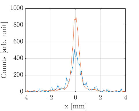
We use the temporal center of the micro-bunches and defocused areas to determine the transverse and longitudinal width of the micro-bunches. A transverse profile of the first micro-bunch of Figure 5 (at $t=28\,\textnormal{ps}$, obtained from Figure 7, averaged over $\pm 0.4\,\textnormal{ps}$) is shown in Figure 8 as an example, demonstrating the typical transverse shape of the micro-bunches. The profiles suggest that there is more charge in the micro-bunch (red line) than in the incoming bunch (blue line) over the same time range. This is not possible, since the proton bunch is strongly relativistic, i.e. protons cannot move longitudinally with respect to each other. This is a good illustration of the slit effect. The micro-bunch width is less that that of the incoming bunch, thus more light is collected through the slit, giving the impression that it contains more charge. Instead, only its charge density is larger (see below).
In order to avoid having to assume a transverse (or longitudinal) profile for the micro-bunches, we plot the running sum of counts over each micro-bunch. For the transverse width we calculate the running sum of counts from the bunch center ($x=0$, Figure 8) to the edge of the image over the time range of each micro-bunch, as determined in Figure 7. We use the time ranges of the micro-bunches of the modulated bunch to calculate the corresponding sums in the unmodulated bunch. Figure 9a) shows the profiles of the unmodulated bunch (Figure 5) for comparison, and Figure 9b) of the modulated bunch (Figure 5). We linearly fit the profiles for $\Delta x>4\,\textnormal{mm}$, corresponding to summation of background, as the light collection from the proton bunch is limited by the imaging aperture. The subtraction of the linear function (dashed lines in Figure 9) leads to saturation of the profiles. We define the bunch width (radius) as the radial position at which the sum reaches $60\%$ of the final value, indicated with the vertical dash-dotted lines. As expected, the width along the unmodulated bunch remains essentially constant, see 9a). For the modulated bunch, 9b) shows the running sum over the micro-bunch number one, four and nine, also representing the shape over the other micro-bunches. Unlike the unmodulated bunch, the width (vertical lines) of the individual micro-bunches is changing along the bunch.

The transverse width of each micro-bunch along the bunch is plotted in Figure 10 (red circles) and compared to the width of the incoming bunch (blue crosses) with a mean of $540\,(\pm$ $20\text{\,}\mathrm{\SIUnitSymbolMicro m}$). One can see that the width of the signal is increasing along the image.

We use a similar approach to determine the length of the micro-bunches, see Figure 11. The micro-bunch length before and after the micro-bunch center here differ from each other and are thus treated individually. We calculate the running sum of counts from the center of the micro-bunch (Figure 7) to its beginning and end (Figure 7). For the given measurement, the bunch is not fully modulated near the ionization front, thus the counts between the micro-bunches do not reach the value 0, i.e. the sums do not saturate. Therefore we limit the range of summation with the beginning (11a) and end (11b) of the micro-bunch and the time of the ionizing laser pulse as the beginning of the first micro-bunch. Here we sum over the transverse range $$-70\text{\,}\mathrm{\SIUnitSymbolMicro m}$<x<$70\text{\,}\mathrm{\SIUnitSymbolMicro m}$$ for a less noisy profile. The vertical dash-dotted lines indicate the determined micro-bunch length, where the sum reaches $60\%$ of the final value.

The lengths are summarized in Figure 12 for each micro-bunch along the bunch. The length from the center to the beginning as blue, from the center to the end as red, and the sum of the two as green crosses. One can see that the first two micro-bunches are longer and after the third micro-bunch the length saturates to $3.1\,(\pm\,0.1)\,\textnormal{ps}$. In the following we use the length of the micro-bunches for the unmodulated bunch for the comparison of charge in a given length along the bunch. Note that temporal resolution might lower the counts per pixel for a signal with time structure, as the modulated bunch, while it should not affect a signal without, as the unmodulated bunch.

We apply this procedure to calculate the charge of the image of the unmodulated (Figure 5) and modulated bunch (Figure 5). To avoid the signal from the timing reference laser pulse we use only half of the image ($x>0$). We compare the charge density summed transversely over the entire modulated bunch (red curve) with the unmodulated bunch (blue curve) in Figure 14. As expected, the shape for the unmodulated bunch follows the Gaussian bunch distribution (with length $\sigma_{\zeta}=300\,\textnormal{ps}$ and $t=0$ being $6\,\textnormal{ps}$ behind the bunch center and amplitude normalized to the measured profile), indicated with the blue dashed line. The summation of the modulated bunch includes focused and defocused protons. Summing the charge density transversely over the bunch before the start of the plasma ($t<24\,\textnormal{ps}$) leads to similar values for the modulated bunch and the incoming bunch, as expected. Summing the charge density transversely over the bunch within the plasma ($t>24\,\textnormal{ps}$) shows significantly lower counts of the modulated bunch than the incoming bunch. The sum of the modulated bunch also exhibits the periodic modulation from the self-modulation process.
The decrease in signal along the image in Figure 14 for the modulated bunch (red curve) is caused by the increase in width (see Figure 10, red circles). We can account for the effect of the slit and determine the charge of the image by multiplying the images containing the charge density with $2\pi\,r\,dr$. Figure 14 shows the sum of the charge over the modulated bunch (red curve) compared to the incoming bunch (blue curve). It shows that the charge along the self-modulated bunch is very close to that of the unmodulated bunch, following the Gaussian profile. The procedure recovers the same charge for parts of the bunch before the plasma ($t<24\,\textnormal{ps}$). However, it retains some of the modulation in the charge density and the recovered charge decreases along the bunch when compared to the incoming bunch charge. These deviations are probably due to light collection and detection limitations of the diagnostic. Protons are more and more defocused along the bunch (see [2]) and images show that they fall out of the imaged field ($-4\,\textnormal{mm}<x<4\,\textnormal{mm}$) later along the bunch. Also, the bunch charge density decreases further along the bunch. The streak camera has a limited signal to noise ratio and low level light is not detected, falling below the detection threshold. The effects increase along the bunch.
Figure 14 shows how well the charge along the bunch can be determined with this diagnostic and procedure. Now, that we have developed a procedure, to recover the charge in the bunch from the measurement of its charge density, and determined its limitation, we can measure the charge carried by each micro-bunch, i.e. not including the charge of defocused protons, and compare it to the incoming charge.

We use the transverse width and length of the incoming bunch and the micro-bunches, as obtained using the procedure detailed in section 2 (Figures 10 and 12), to determine the relative charge per micro-bunch. For comparison of the charge in each micro-bunch with the charge in the incoming bunch, we use the same time ranges for the summation on the images of the modulated and unmodulated bunch.
Summation of the charge density, as given by the original streak camera image, over the range of the micro-bunches, is shown in Figure 16. The image of the unmodulated bunch, where the squares indicate the transverse width of the unmodulated bunch and the length of the micro-bunches, is shown in a); the image of the modulated bunch, with the ellipses of the width and length of the micro-bunches in b). In c) the charge density summed over the squared areas in a) (blue crosses) and over the ellipses in b) (red circles) is shown. One can see that the summed charge density for the unmodulated bunch remains essentially constant (considering the limitation of this procedure, the longitudinal bunch position close to the center, and the difference in length for the first micro-bunches and thus summation length being small). In constrast, the summed charge density of the micro-bunches decreases rapidly along the bunch, due to the increasing radial size of the signal (see Figure 10). This is consistent with Figure 14, where the charge density of the unmodulated bunch follows the Gaussian bunch distribution, while the charge density of the modulated bunch decreases along the bunch.
In order to determine the charge per micro-bunch we multiply the streak camera images $n(r,t)$ by $2\pi\,r\,dr$, as shown in Figure 16a) for the unmodulated and b) for the modulated bunch. We sum over the same squares and ellipses as described above, in order to determine the charge per micro-bunch. Figure c) compares the charge per micro-bunch with the charge of the incoming bunch. Again, we expect the charge of the unmodulated bunch to be essentially constant (central position within the long Gaussian bunch and small changes in micro-bunch length), which is confirmed by the measurement in blue. In red it is demonstrated that also the charge per micro-bunch is roughly constant along the bunch. The mean charge per micro-bunch covered in the ellipse is $64\,(\pm\,9)\%$ of the charge covered in the squares of the incoming bunch.

References

- [1] P. Muggli et al. (AWAKE Collaboration), Plasma Physics and Controlled Fusion, 60(1) 014046 (2017).
- [2] M. Turner et al. (AWAKE Collaboration), Phys. Rev. Lett. 122, 054801 (2019).
- [3] E. Adli et al. (AWAKE Collaboration), Phys. Rev. Lett. 122, 054802 (2019).
- [4] E. Adli et al. (AWAKE Collaboration), Nature 561, 363–367 (2018).
- [5] K. Rieger et al., Rev. of Scientific Instruments 88, 025110 (2017).
- [6] F. Batsch et al., submitted for EAAC2019 proceedings, arXiv:1911.12201.