Distance to the stochastic part of phylogenetic varieties

Marta Casanellas , Jesús Fernández-Sánchez and Marina Garrote-López

Abstract.

Modelling the substitution of nucleotides along a phylogenetic tree is usually done by a hidden Markov process. This allows to define a distribution of characters at the leaves of the trees and one might be able to obtain polynomial relationships among the probabilities of different characters. The study of these polynomials and the geometry of the algebraic varieties defined by them can be used to reconstruct phylogenetic trees. However, not all points in these algebraic varieties have biological sense. In this paper, we explore the extent to which adding semi-algebraic conditions arising from the restriction to parameters with statistical meaning can improve existing methods of phylogenetic reconstruction. To this end, our aim is to compute the distance of data points to algebraic varieties and to the stochastic part of these varieties. Computing these distances involves optimization by nonlinear programming algorithms. We use analytical methods to find some of these distances for quartet trees evolving under the Kimura 3-parameter or the Jukes-Cantor models. Numerical algebraic geometry and computational algebra play also a fundamental role in this paper.

Keywords. Phylogenetic variety; Euclidean distance degree; semi-algebraic phylogenetics; group-based models; quartet topology; long-branch attraction

1. Introduction

Within the new century, algebraic tools have started to be successfully applied to some problems of phylogenetic reconstruction, see for example Allman et al. 2013, Chifman and Kubatko 2015 and Allman et al. 2017. The main goal of phylogenetic reconstruction is to estimate the phylogenetic tree that best explains the evolution of living species using solely information of their genome. To this end, one usually considers evolutionary models of molecular substitution and assume that DNA sequences evolve according to these models by a Markov process on a tree. Some of the most used models are nucleotide substitution models (e.g. Kimura 1981 or Jukes and Cantor 1969 models), which are specified by a $4\times 4$ transition matrix associated to each edge of the tree and a distribution of nucleotides at the root. Then, the distribution of possible nucleotide sequences at the leaves of the tree (representing the living species) can be computed as an algebraic expression in terms of the parameters of the model (the entries of the substitution matrices and the distribution at the root). This allows the use of algebraic tools for phylogenetic reconstruction purposes.

When reconstructing the tree topology (i.e., the shape of the tree taking into account the names of the species at the leaves), the main tools that have been used come either from rank conditions on matrices arising from a certain rearrangement of the distribution of nucleotides at the leaves (Chifman and Kubatko 2014; Chifman and Kubatko 2015; Casanellas and Fernández-Sánchez 2016), or from phylogenetic invariants (Lake 1987; Casanellas and Fernández-Sánchez 2007). These tools use the fact that the set of possible distributions satisfies certain algebraic constraints, but do not specifically use the condition that one is dealing with discrete distributions that arise from stochastic matrices at the edges of the tree (i.e. with positive entries and rows summing to one). These extra conditions lead to semi-algebraic constraints which have been specified for certain models by Allman et al. 2012 (for the general Markov model), Matsen 2009 (for the Kimura 3-parameter model) and by Zwiernik and Smith 2011 and Klaere and Liebscher 2012 for the 2-state case ( $2\times 2$ transition matrices). Combining algebraic and semi-algebraic conditions to develop a tool for reconstructing the tree topology is not an easy task and, as far as we are aware, both tools have only been used together in Kosta and Kubjas 2019 for the simple case of 2 states.

As a starting point of topology reconstruction problems, it is natural to use trees on four species (called 1, 2, 3, 4 for example). In this case, there are three possible (unrooted and fully resolved) phylogenetic trees, $13|24$ , $13|24$ , and $14|23$ (see Fig. 1). Then a distribution of nucleotides for this set of species is a vector $P\in\mathbb{R}^{4^{4}}$ whose entries are non-negative and sum to one. The set of distributions arising from a Markov process on any of these trees $T$ (for a given substitution model) defines an algebraic variety $\mathcal{V}_{T}$ (see Section 2.1). The three phylogenetic varieties $\mathcal{V}_{12|34}$ , $\mathcal{V}_{13|24}$ , $\mathcal{V}_{14|23}$ are different and the topology reconstruction problem for a given distribution $P\in\mathbb{R}^{4^{4}}$ is, briefly, deciding to which of these three varieties $P$ is closest (for a certain distance or for another specified optimization problem such as likelihood estimation). The algebraic tools related to rank conditions mentioned above attempt to estimate these Euclidean distances, for example.

Refer to caption — Figure 1. The three unrooted (fully resolved) phylogenetic trees on $4$ leaves: $12|34$ (left), $13|24$ (middle) and $14|23$ (right).

If we assume that $P$ should be close to a distribution that has arisen from stochastic parameters on one of these trees, then one should consider only the stochastic part of these varieties, $\mathcal{V}_{12|34}^{+}$ , $\mathcal{V}_{13|24}^{+}$ , $\mathcal{V}_{14|23}^{+}$ (which we call the stochastic phylogenetic regions). The main questions that motivated the study presented here are:

-

Could semi-algebraic tools add some insight to the already existent algebraic tools?
-

Do semi-algebraic conditions support the same tree $T$ whose algebraic variety $\mathcal{V}_{T}$ is closest to the data point?

In terms of the Euclidean distance and trees of four species, we make the explicit following question:

(*)

If $P\in\mathbb{R}^{4^{4}}$ is a distribution satisfying $d(P,\mathcal{V}_{12|34})<min\{d(P,\mathcal{V}_{13|24}),d(P,\mathcal{V}_{14|23})\}$ , would it be possible that $d(P,\mathcal{V}_{12|34}^{+})>\min\{d(P,\mathcal{V}_{13|24}^{+}),d(P,\mathcal{V}_{14|23}^{+})\}$ ?

We address this problem for special cases of interest in phylogenetics: short branches at the external edges (see section 4) and long branch attraction (in section 6). The length of a branch in a phylogenetic tree is understood as the expected number of substitutions of nucleotides per site along the corresponding edge; both cases, short and long branches, usually lead to confusing results in phylogenetic reconstruction (particularly in relation to the long branch attraction problem, see section 6). In the first case we are able to deal with the Kimura 3-parameter model and in the second case we have to restrict to the more simple Jukes-Cantor (JC69) model. The reason for this restriction is that the computations get more involved in the second case and we have to use computational algebra techniques (for which is crucial to decrease the number of variables of the problem). To this end, in section 5 we introduce an algorithm that computes the distance of a point to the stochastic phylogenetic regions in the JC69 case; this algorithm makes explicit use of the Euclidean distance degree (Draisma et al. 2015) of the phylogenetic varieties.

We find that in the first framework (short external branches), restricting to the stochastic part does not make any difference, that is, Question 1 has a negative answer in this case (see Theorem 4.3). However, in the long branch attraction framework, considering the stochastic part of phylogenetic varieties might be of interest, specially if the data points are close to the intersection of the three varieties, see Theorem 6.6. In particular, the answer to Question 1 is positive for data close to the long branch attraction problem under the JC69 model. In section 7 we provide results on simulated data that support these findings and also show a positive answer to Question 1 for balanced trees.

Summing up, incorporating the semi-algebraic conditions to the problem of phylogenetic reconstruction seems important when the data are close to the intersection of the three phylogenetic varieties. This is the case where phylogenetic reconstruction methods tend to confuse the trees. On the contrary, on data points which are far from the intersection (in the short branches case of section 4 for example), it does not seem necessary to incorporate these semi-algebraic tools. This is the reason why incorporating these tools into phylogenetic reconstruction methods might be extremely difficult.

In this paper we consider only the Euclidean distance. One reason to do so is that the initial algebraic tools based on rank conditions were dealing with it, but another motivation is that the algebraic expression of the Euclidean distance permits the use of algebraic tools to derive analytical results and the use of numerical algebraic geometry to get global minima. On the other hand, the use of other measures such as Hellinger distance or maximum likelihood, would not allow the use of the Fourier transform for the evolutionary models we use here, which significantly simplifies the computations in our case.

The organization of the paper is as follows. In section 2, we introduce the concepts on nucleotide substitution models and phylogenetic varieties that we will use later on. Then in section 3 we prove some technical results regarding the closest stochastic matrix to a given matrix. In section 4 we consider the case of short external branches for the Kimura 3-parameter model and obtain the results analytically. In section 5 we introduce the computational approach that we use in order to compute the distance to the stochastic phylogenetic regions. The results for the long branch attraction case are expanded in section 6 and in section 7 we provide results on simulated data that illustrate our findings. The Appendix collects all technical proofs needed in section 6.

2. Preliminaries

2.1. Phylogenetic varieties

We refer the reader to the work by Allman and Rhodes 2007 for a good general overview of phylogenetic algebraic geometry. Here we briefly introduce the basic concepts that will be needed later. Let $T$ be a quartet tree topology, that is, an (unrooted) trivalent phylogenetic tree with its leaves labelled by $\{1,2,3,4\}$ (i.e. $T$ is a connected acyclic graph whose interior nodes have degree $3$ and whose leaves, of degree 1, are in correspondence with $\{1,2,3,4\}$ ), see Fig. 1. Using the notation introduced in Fig. 1, $T$ belongs to the set $\mathcal{T}=\{12|34,13|24,14|23\}$ . We choose an internal vertex as the root $r$ of $T$ , which induces an orientation on the set of edges $E(T)$ . Suppose the Markovian evolutionary process on that tree follows a nucleotide substitution model $\mathcal{M}$ : associate a random variable taking values on $\Sigma:=\{\mathtt{A},\mathtt{C},\mathtt{G},\mathtt{T}\}$ at each node of the tree, and consider as parameters a distribution $\pi=(\pi_{\mathtt{A}},\pi_{\mathtt{C}},\pi_{\mathtt{G}},\pi_{\mathtt{T}})$ at the root, $\sum_{i}\pi_{i}=1$ , and a $4\times 4$ transition matrix $M_{e}$ at each (oriented) edge $e$ of $T$ . The transition matrices are stochastic (or Markov) matrices, that is, all its entries are non-negative and its rows sum up to $1$ . A vector is stochastic if all its entries are nonnegative and sum up to $1$ .

If $T\in\mathcal{T}$ and $S$ is the set of stochastic parameters described above, we denote by $\psi_{T}$ the following (parametrization) map:

	$\displaystyle\psi_{T}:S\subset[0,1]^{\ell}$	$\displaystyle\rightarrow\mathbb{R}^{4^{4}}$
	$\displaystyle\{\pi,\{M_{e}\}_{e\in E(T)}\}$	$\displaystyle\mapsto P=(p_{\mathtt{AAAA}},p_{\mathtt{AAAC}},\ldots,p_{\mathtt{TTTG}},p_{\mathtt{TTTT}})$

which maps each set of parameters of the model $\{\pi,\{M_{e}\}_{e\in E(T)}\}\in S$ to the joint distribution of characters at the leaves of $T$ given by a hidden Markov process on $T$ governed by these parameters. The entries $p_{x_{1},\ldots,x_{4}}$ of the joint distribution can be expressed in terms of the entries of the substitution matrices. We adopt the following notation: trees are rooted at the interior node neighbour to leaf 1, for $i=1,\ldots,4$ , $M_{i}$ is the transition matrix on the edge ending at leaf $i$ , and $M_{5}$ is the transition matrix at the interior edge. For example, for the tree $12|34$ rooted at the leftmost internal edge with transition matrices as in Fig. 2 we have

p_{x_{1},x_{2},x_{3},x_{4}}=\sum_{x_{r},x_{s}\in\Sigma}\pi_{x_{r}}M_{1}(x_{r},x_{1})M_{2}(x_{r},x_{2})M_{5}(x_{r},x_{s})M_{3}(x_{s},x_{3})M_{4}(x_{s},x_{5}).

We write $\mathcal{V}_{T}^{+}$ for the image of this map, that is, the space of all the distributions arising from stochastic parameters,

\mathcal{V}_{T}^{+}=\{P\in\mathcal{V}_{T}\ |\ P=\psi_{T}(s)\mbox{ and }s\in S\}.

We call this set the stochastic phylogenetic region.

Since $\psi_{T}$ is a polynomial map, it can be extended to $\mathbb{R}^{\ell}$ . That is, we can consider not only nonnegative entries in $\pi$ and $M_{e}$ , but we always assume that the rows of the matrices $M_{e}$ and the vector $\pi$ , sum up to $1$ . Define the phylogenetic variety associated with $\mathcal{T}$ as the Zariski closure of $\psi_{T}(\mathbb{R}^{l})$ ,

\mathcal{V}_{T}=\overline{\psi_{T}(\mathbb{R}^{l})}.

This variety contains all joint distributions that arise from stochastic parameters on the tree $T$ , but not every point in this variety is of this type.

Although the choice of a root was necessary to define the map $\psi_{T}$ , the phylogenetic variety and the stochastic region do not depend on it (Allman and Rhodes 2003). Throughout the paper we consider the Euclidean distance between points, even if we do not specify it.

2.2. Kimura and Jukes-Cantor models

In this paper we focus on phylogenetic $4$ -leaf trees evolving under the Jukes-Cantor model ( $JC69$ for short, see Jukes and Cantor 1969) and also the $3$ -parameter Kimura model ( $K81$ for short, see Kimura 1981). The JC69 model is a highly structured model that assumes equal mutation probabilities and the K81 takes into account the classification of nucleotides as purines/pyrimidines and the probabilities of substitution between and within these groups; both models assume the uniform distribution at the root, $\pi=(\frac{1}{4},\frac{1}{4},\frac{1}{4},\frac{1}{4})$ .

Definition 2.1.

A $4\times 4$ matrix $M$ is a K81 matrix if it is of the form

(1)

\footnotesize M=\left(\begin{array}[]{c@{\quad}c@{\quad}c@{\quad}c}a\hfil\hskip 8.50012pt&b\hfil\hskip 8.50012pt&c\hfil\hskip 8.50012pt&d\\ b\hfil\hskip 8.50012pt&a\hfil\hskip 8.50012pt&d\hfil\hskip 8.50012pt&c\\ c\hfil\hskip 8.50012pt&d\hfil\hskip 8.50012pt&a\hfil\hskip 8.50012pt&b\\ d\hfil\hskip 8.50012pt&c\hfil\hskip 8.50012pt&b\hfil\hskip 8.50012pt&a\\ \end{array}\right),

for some $a,b,c,d\in\mathbb{R}$ summing to 1, $a+b+c+d=1$ . If $b=c=d$ , then we say that $M$ is a JC69 matrix.

Note that these matrices only have an interpretation as transition matrices of a Markov process if they have nonnegative entries; in this case we talk about stochastic K81 matrices or stochastic JC69 matrices.

Lemma 2.2.

(Allman and Rhodes 2004a) If $M$ is a $K81$ matrix as (1), then it diagonalizes with eigenvalues $m_{\mathtt{A}}=a+b+c+d=1$ , $m_{\mathtt{C}}=a+b-c-d$ , $m_{\mathtt{G}}=a-b+c-d$ and $m_{\mathtt{T}}=a-b-c+d$ and respective eigenvectors $\bar{\mathtt{A}}=(1,1,1,1)^{t}$ , $\bar{\mathtt{C}}=(1,1,-1,-1)^{t}$ , $\bar{\mathtt{G}}=(1,-1,1,-1)^{t}$ and $\bar{\mathtt{T}}=(1,-1,-1,1)^{t}$ . In particular, the eigenvalues of a $JC69$ matrix are $m_{\mathtt{A}}=1$ and $m_{\mathtt{C}}=m_{\mathtt{G}}=m_{\mathtt{T}}=1-4b$ .

2.3. Fourier coordinates and Fourier parameters

Let $M$ be a $K81$ matrix and write $m_{\mathtt{A}},m_{\mathtt{C}},m_{\mathtt{G}},m_{\mathtt{T}}$ and $\bar{\mathtt{A}},\bar{\mathtt{C}},\bar{\mathtt{G}},\bar{\mathtt{T}}$ for the eigenvalues and eigenvectors of $M$ , respectively. The basis of eigenvectors will be denoted by $\hbox to0.0pt{\hskip 1.1111pt\hbox{$\overline{\hbox{}}$}\hss}{\hbox{$\Sigma$}}=\{\bar{\mathtt{A}},\bar{\mathtt{C}},\bar{\mathtt{G}},\bar{\mathtt{T}}\}$ and is called the Fourier basis. Because of Lemma 2.2, we have

\displaystyle\hbox to0.0pt{\hskip 2.89581pt\hbox{$\overline{\hbox{}}$}\hss}{\hbox{$M$}}=H^{-1}\cdot M\cdot H,

where $\hbox to0.0pt{\hskip 2.89581pt\hbox{$\overline{\hbox{}}$}\hss}{\hbox{$M$}}=diag(m_{\mathtt{A}},m_{\mathtt{C}},m_{\mathtt{G}},m_{\mathtt{T}})$ and

\footnotesize H=\left(\begin{array}[]{c@{\quad}c@{\quad}c@{\quad}c}1\hfil\hskip 8.50012pt&1\hfil\hskip 8.50012pt&1\hfil\hskip 8.50012pt&1\\ 1\hfil\hskip 8.50012pt&1\hfil\hskip 8.50012pt&-1\hfil\hskip 8.50012pt&-1\\ 1\hfil\hskip 8.50012pt&-1\hfil\hskip 8.50012pt&1\hfil\hskip 8.50012pt&-1\\ 1\hfil\hskip 8.50012pt&-1\hfil\hskip 8.50012pt&-1\hfil\hskip 8.50012pt&1\\ \end{array}\right)

is the matrix of change of basis from $\overline{\hbox{}}$ $\Sigma$ to $\Sigma$ . Notice that $H^{-1}=\frac{1}{4}H^{t}=\frac{1}{4}H$ . The eigenvalues $m^{i}_{\mathtt{A}},m^{i}_{\mathtt{C}},m^{i}_{\mathtt{G}},m^{i}_{\mathtt{T}}$ of $M_{i}$ will be called Fourier parameters.

The vectors $P=(p_{\mathtt{AAAA}},p_{\mathtt{AAAC}},\ldots,p_{\mathtt{TTTG}},p_{\mathtt{TTTT}})\in\mathbb{R}^{4^{4}}$ considered in section 2.1 can be thought of as $4\times 4\times 4\times 4$ tensors in $\left(\mathbb{R}^{4}\right)^{\otimes 4}$ : if we call $\Sigma=\{\mathtt{A},\mathtt{C},\mathtt{G},\mathtt{T}\}$ the standard basis of $\mathbb{R}^{4}$ , then the components $p_{x_{1}x_{2}x_{3}x_{4}}$ of $P$ are its coordinates in the natural basis in $\otimes^{4}\mathbb{R}^{4}$ induced by $\Sigma$ . This motivates the following definition.

Definition 2.3.

Given a tensor $P$ in $\left(\mathbb{R}^{4}\right)^{\otimes 4}$ , we denote by $(p_{\mathtt{AAAA}},p_{\mathtt{AAAC}},\ldots,p_{\mathtt{TTTT}})^{t}$ the coordinates of $P$ in the basis $\{\mathtt{A\otimes A\otimes A\otimes A},\mathtt{A\otimes A\otimes A\otimes C},\mathtt{\ldots},\mathtt{T\otimes T\otimes T\otimes T}\}$ induced by $\Sigma$ . Similarly, we write $\hbox to0.0pt{\hskip 1.40451pt\hbox{$\overline{\hbox{}}$}\hss}{\hbox{$P$}}=(\bar{p}_{\mathtt{AAAA}},\bar{p}_{\mathtt{AAAC}},\ldots,\bar{p}_{\mathtt{TTTG}},\bar{p}_{\mathtt{TTTT}})^{t}$ for the coordinates of $P$ in the basis $\{\mathtt{\bar{A}\otimes\bar{A}\otimes\bar{A}\otimes\bar{A}},\mathtt{\ldots},\mathtt{\bar{T}\otimes\bar{T}\otimes\bar{T}\otimes\bar{T}}\}$ induced by the Fourier basis $\overline{\hbox{}}$ $\Sigma$ .

The relation between the natural coordinates and the Fourier coordinates of $P$ is:

\displaystyle\hbox to0.0pt{\hskip 1.40451pt\hbox{$\overline{\hbox{}}$}\hss}{\hbox{$P$}}=\left(H^{-1}\otimes H^{-1}\otimes H^{-1}\otimes H^{-1}\right)P=\frac{1}{4^{4}}\left(H\otimes H\otimes H\otimes H\right)P.

Remark 2.4.

Since $\frac{1}{2}H$ is an orthogonal matrix, so is $U:=\left(\frac{1}{2}H\right)\otimes\left(\frac{1}{2}H\right)\otimes\left(\frac{1}{2}H\right)\otimes\left(\frac{1}{2}H\right)$ . Therefore,

\displaystyle\parallel{\hbox to0.0pt{\hskip 1.40451pt\hbox{$\overline{\hbox{}}$}\hss}{\hbox{$P$}}-\hbox to0.0pt{\hskip 1.45276pt\hbox{$\overline{\hbox{}}$}\hss}{\hbox{$Q$}}}\parallel^{2}

\displaystyle=\parallel{\frac{1}{2^{4}}U{P}-\frac{1}{2^{4}}U{Q}}\parallel^{2}=\frac{1}{4^{4}}\parallel P-Q\parallel^{2}

and the Euclidean distance between tensors can be computed using the Fourier coordinates (up to a positive scalar): $d({P},{Q})=16||\hbox to0.0pt{\hskip 1.40451pt\hbox{$\overline{\hbox{}}$}\hss}{\hbox{$P$}}-\hbox to0.0pt{\hskip 1.45276pt\hbox{$\overline{\hbox{}}$}\hss}{\hbox{$Q$}}||$ .

If one considers the following bijection between $\Sigma$ and the group $G:(\mathbb{Z}/2\mathbb{Z}\times\mathbb{Z}/2\mathbb{Z},+)$ ,

\begin{array}[]{ccc}\Sigma=\{\mathtt{A},\mathtt{C},\mathtt{G},\mathtt{T}\}&\longleftrightarrow&\mathbb{Z}/2\mathbb{Z}\times\mathbb{Z}/2\mathbb{Z}\\ \mathtt{A}&\mapsto&(0,0)\\ \mathtt{C}&\mapsto&(0,1)\\ \mathtt{G}&\mapsto&(1,0)\\ \mathtt{T}&\mapsto&(1,1)\\ \end{array},

then the previous change of coordinates can be understood as the discrete Fourier transform on $G^{4}$ . The following result states that the polynomial parametrization $\psi_{T}$ becomes monomial in the Fourier parameters:

Theorem 2.5.

(Evans and Speed 1993) Let $P=\psi_{T}(\pi,\{M_{i}\}_{i\in[5]})$ where $T$ is the tree topology $A|B$ and $M_{i}$ are $K81$ matrices. If $m_{\mathtt{A}}^{i},m_{\mathtt{C}}^{i},m_{\mathtt{G}}^{i},m_{\mathtt{T}}^{i}$ are the Fourier parameters of $M_{i}$ , then the Fourier coordinates of $P$ are

\bar{p}_{x_{1}x_{2}x_{3}x_{4}}=\begin{cases}\frac{1}{4^{4}}m_{\mathtt{x_{1}}}^{1}m_{\mathtt{x_{2}}}^{2}m_{\mathtt{x_{3}}}^{3}m_{\mathtt{x_{4}}}^{4}m_{\sum_{i\in A}\mathtt{x_{i}}}^{5}&\text{if $\sum_{i\in A}{\mathtt{x_{i}}}=\sum_{j\in B}{\mathtt{x_{j}}}$,}\\ 0&\text{otherwise,}\end{cases}

where the sum of elements in $\Sigma$ is given by the bijection $\Sigma\leftrightarrow\mathbb{Z}/2\mathbb{Z}\times\mathbb{Z}/2\mathbb{Z}$ introduced above.

Notation 2.6.

From now on, for the JC69 model, we denote by $x_{i}$ the eigenvalue of $M_{i}$ of multiplicity three different from 1 (see Lemma 2.2) and we denote by $\varphi_{T}$ the parameterization of the phylogenetic varieties from Fourier parameters to Fourier coordinates,

\begin{array}[]{rcl}\varphi_{T}:\mathbb{R}^{5}&\longrightarrow&\mathbb{R}^{4^{4}}\\ \mathbf{x}=(x_{1},x_{2},x_{3},x_{4},x_{5})&\mapsto&\hbox to0.0pt{\hskip 1.40451pt\hbox{$\overline{\hbox{}}$}\hss}{\hbox{$P$}}=\varphi_{T}(x_{1},x_{2},x_{3},x_{4},x_{5}).\end{array}

The parametrization $\varphi_{T}$ can be computed by adapting Theorem 2.5 to this model.

3. The closest stochastic matrix

Throughout this section, we will use the following notation. We write $\mathcal{H}$ for the hyperplane $\{x_{1}+\ldots+x_{N}=1\}\subset\mathbb{R}^{N}$ and $\Delta:=\{(x_{1},\ldots,x_{N})\mid\sum_{i}x_{i}=1,x_{i}\geq 0\}$ for the standard simplex in $\mathbb{R}^{N}$ . Given a point $\mathbf{x}\in\mathbb{R}^{N}$ , we denote by $\proj_{\mathcal{H}}(\mathbf{x})$ its orthogonal projection onto $\mathcal{H}$ .

Definition 3.1.

For any matrix $M\in\mathcal{M}_{N}(\mathbb{R})$ we denote by $\widehat{M}$ its closest stochastic matrix in the Frobenious norm:

\widehat{M}=\argmin_{\begin{subarray}{c}\sum_{j}X_{ij}=1\ \forall i,\\ X_{ij}\geq 0\ \forall(i,j)\end{subarray}}\parallel M-X\parallel_{F}.

Similarly, for any point $\mathbf{x}\in\mathbb{R}^{N}$ we write $\widehat{\mathbf{x}}$ for its closest point in $\Delta$ .

The problem of finding the nearest stochastic matrix is equivalent to finding the closest point (in Euclidean norm) in the standard simplex to every row of the matrix Kreinin and Sidelnikova 2001. The uniqueness of $\widehat{v}$ , and consequently of $\widehat{M}$ , is guaranteed since both the objective function and the domain set are convex. The problem of finding the closest point in the simplex $\Delta$ to a given point has been widely studied and there exist several algorithms to compute it. 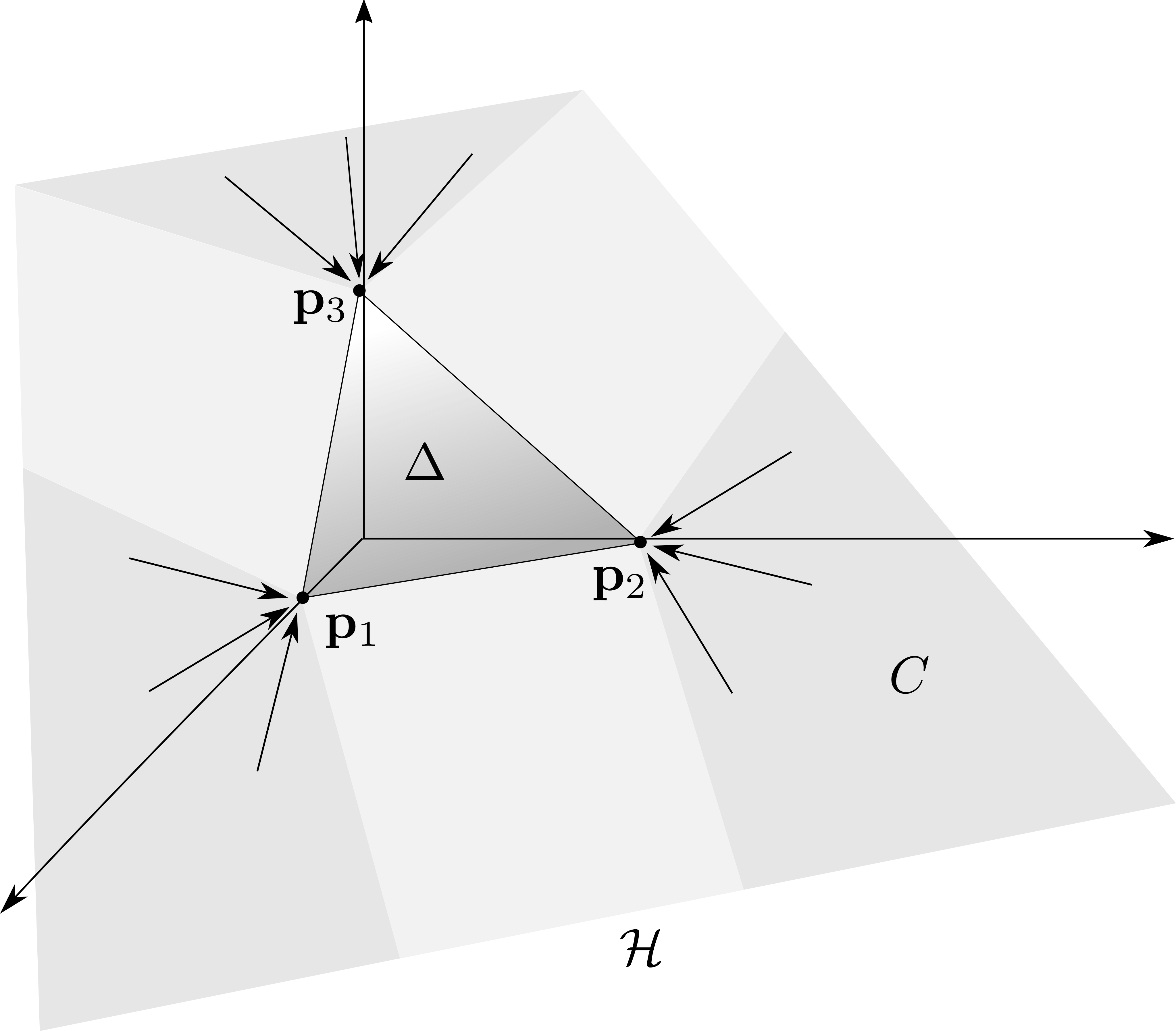We refer the reader to the work by Michelot 1986 for an algorithm that, given any point $\mathbf{x}\in\mathbb{R}^{N}$ , produces the point $\widehat{\mathbf{x}}\in\Delta$ that minimizes $\parallel\mathbf{x}-\mathbf{y}\parallel_{2}$ for $\mathbf{y}\in\Delta$ .

In the following result we state some properties that will be useful later (see Fig. 3 for an illustration of the last item).

Lemma 3.2.

Let $\mathbf{x}=(x_{1},\ldots,x_{N})$ be a point in $\mathbb{R}^{N}$ and let $\widehat{\mathbf{x}}=(\widehat{x}_{1},\ldots,\widehat{x}_{N})$ be its closest point in $\Delta$ .

(i)

$\widehat{\mathbf{x}}$ coincides with the closest point to $\proj_{\mathcal{H}}(\mathbf{x})$ in $\Delta$ , $\widehat{\proj_{\mathcal{H}}(\mathbf{x}).}$
(ii)

If $\mathbf{x}\in\mathcal{H}$ and $x_{i}\leq 0$ for some $i$ , then $\widehat{x}_{i}=0$ .
(iii)

Let $\mathbf{y}$ be a point obtained by a permutation of the coordinates of $\mathbf{x}$ , i.e. $\mathbf{y}=P\mathbf{x}$ for some permutation matrix $P$ . Then $\widehat{\mathbf{y}}=P\widehat{\mathbf{x}}$ .
(iv)

If $x_{i}=x_{j}$ for some $i,j=1,\ldots,N$ then $\widehat{x}_{i}=\widehat{x}_{j}$ .
(v)

$\widehat{\mathbf{x}}$ coincides with $\mathbf{p}_{i}=(0,\ldots,\underset{\begin{subarray}{c}\frown\vskip-1.9919pt\\ i\end{subarray}}{1},\ldots,0)$ if and only if $x_{i}-x_{j}\geq 1$ $\forall j\neq i$ .

Proof.

The proofs of items $(i)$ and $(ii)$ can be found in the paper by Michelot 1986 and are the basis of the algorithm provided there.

$(iii)$ It follows from the fact that $P$ is a permutation matrix and hence is an orthogonal matrix.

$(iv)$ This is a direct consequence of $(iii)$ .

$(v)$ Using $(i)$ and $(ii)$ we can assume that $\sum_{i}x_{i}=1$ , i.e., $\mathbf{x}$ belongs to the affine hyperplane $\mathcal{H}$ . By symmetry, it is enough to prove the result for $\mathbf{p}_{1}$ , that is, we prove that $\widehat{\mathbf{x}}=\mathbf{p}_{1}$ if and only if $x_{1}-x_{j}\geq 1$ for all $j\neq 1$ . Firstly we show that if $x_{1}-x_{j}\geq 1$ , $j\neq 1$ , then necessarily $\widehat{\mathbf{x}}=\mathbf{p}_{1}$ . Indeed, if $\mathbf{q}=(c_{1},\ldots,c_{N})\in\Delta$ , we have that

(2)		$\displaystyle d(\mathbf{x},\mathbf{q})^{2}$	$\displaystyle=$	$\displaystyle\sum_{j=1}^{N}x_{j}^{2}+\left(\sum_{j=1}^{N}c_{j}^{2}-2\sum_{j=1}^{N}c_{j}x_{j}\right)$
	$\displaystyle d(\mathbf{x},\mathbf{p}_{1})^{2}$	$\displaystyle=$	$\displaystyle\sum_{j=1}^{N}x_{j}^{2}+(1-2x_{1}).$

Now, because of the assumption $x_{1}-x_{j}\geq 1$ and $\sum_{j}c_{j}=1$ , we have that

\displaystyle\sum_{j=1}^{N}c_{j}x_{j}\leq\sum_{j=1}^{N}c_{j}x_{1}-\big(\sum_{j=2}^{N}c_{j}\big)=x_{1}+(c_{1}-1).

In particular,

\displaystyle\sum_{j=1}^{N}c_{j}^{2}-2\sum_{j=1}^{N}c_{j}x_{j}\geq\sum_{j=1}^{N}c_{j}^{2}-2(x_{1}+c_{1}-1)=(c_{1}-1)^{2}+\sum_{j=2}^{N}c_{j}^{2}+(1-2\,x_{1})\geq 1-2\,x_{1}.

Comparing this with (2), it follows that $d(\mathbf{x},q)\geq d(\mathbf{x},\mathbf{p}_{1})$ for any $q\in\Delta$ , so $\mathbf{p}_{1}=\widehat{\mathbf{x}}$ . Conversely, assume that $\mathbf{x}\in\mathcal{H}$ is such that $x_{1}-x_{i}<1$ for some $i\geq 2$ . We will show that there exists some $\mathbf{q}$ in the edge $\mathbf{p}_{1}\mathbf{p}_{i}$ such that $d(\mathbf{x},\mathbf{q})<d(\mathbf{x},\mathbf{p}_{1})$ so that $\mathbf{p}_{1}$ cannot be the closest point to $\mathbf{x}$ in the simplex $\Delta$ . Consider $\mathbf{q}=a\mathbf{p}_{1}+b\mathbf{p}_{i}$ with $a,b\geq 0$ , $a+b=1$ . As above, we have that

\displaystyle d(\mathbf{x},\mathbf{q})^{2}

\displaystyle=

\displaystyle\sum_{j=1}^{N}x_{j}^{2}+a^{2}-2\,a\,x_{1}+b^{2}-2\,b\,x_{i}.

We claim that if we take $0<b<1+x_{i}-x_{1}$ , then the point $\mathbf{q}$ satisfies the inequality between distances above. Indeed, we need to verify that

\displaystyle a^{2}-2\,a\,x_{1}+b^{2}-2\,b\,x_{i}<1-2x_{1}=(a+b)^{2}-2x_{1}=a^{2}+b^{2}+2ab-2x_{1}.

Using that $a=1-b$ , this is equivalent to the inequality $b(b-1+x_{1}-x_{i})<0$ , which is satisfied by our choice of $b$ . ∎

Remark 3.3.

If the rows of a matrix $M$ are the result of some permutation applied to the first row, the previous lemma shows that $\widehat{M}$ will preserve the same identities between entries as the matrix $M$ . Actually, it can be shown that if $M$ is a matrix in an equivariant model (Draisma and Kuttler 2009), then $\widehat{M}$ will remain in the same model. For example, the matrix

\displaystyle\footnotesize M=\left(\begin{array}[]{c@{\quad}c@{\quad}c@{\quad}c}0.9\hfil\hskip 8.50012pt&0.03\hfil\hskip 8.50012pt&-0.01\hfil\hskip 8.50012pt&0.08\\ 0.03\hfil\hskip 8.50012pt&0.9\hfil\hskip 8.50012pt&0.08\hfil\hskip 8.50012pt&-0.01\\ -0.01\hfil\hskip 8.50012pt&0.08\hfil\hskip 8.50012pt&0.9\hfil\hskip 8.50012pt&0.03\\ 0.08\hfil\hskip 8.50012pt&-0.01\hfil\hskip 8.50012pt&0.03\hfil\hskip 8.50012pt&0.9\\ \end{array}\right)

is a non-stochastic K81 matrix (see (1)). Its nearest stochastic matrix is

\displaystyle\footnotesize\widehat{M}=\left(\begin{array}[]{c@{\quad}c@{\quad}c@{\quad}c}{0.89\wideparen{6}}\hfil\hskip 8.50012pt&0.02\wideparen{6}\hfil\hskip 8.50012pt&0\hfil\hskip 8.50012pt&0.07\wideparen{6}\\ {0.02\wideparen{6}}\hfil\hskip 8.50012pt&{0.89\wideparen{6}}\hfil\hskip 8.50012pt&{0.07\wideparen{6}}\hfil\hskip 8.50012pt&0\\ 0\hfil\hskip 8.50012pt&{0.07\wideparen{6}}\hfil\hskip 8.50012pt&{0.89\wideparen{6}}\hfil\hskip 8.50012pt&{0.02\wideparen{6}}\\ {0.07\wideparen{6}}\hfil\hskip 8.50012pt&0\hfil\hskip 8.50012pt&{0.02\wideparen{6}}\hfil\hskip 8.50012pt&{0.89\wideparen{6}}\\ \end{array}\right).

and preserves the same identities between entries. That is, $\widehat{M}$ remains in the K81 model.

Lemma 3.4.

Let $M$ be a $JC69$ matrix. Then $M$ is stochastic if and only if its eigenvalues lie in $\left[-1/3,1\right]$ .

Proof.

Let $M$ be a JC69 matrix, that is, $M$ as in (1) with $c=d=b$ , $a=1-3b$ . Then, $M$ is stochastic if and only if $b\geq 0$ and $a=1-3b\geq 0$ , which is equivalent to $b\in[0,1/3]$ . As the eigenvalues of $M$ are $m_{\mathtt{A}}=1$ and $m_{\mathtt{C}}=m_{\mathtt{G}}=m_{\mathtt{T}}=1-4b$ (see Lemma 2.2), we get that $M$ is stochastic if and only if the eigenvalue $1-4b$ lies in $[-1/3,1]$ . ∎

Lemma 3.5.

Let $M$ be a non-stochastic JC69 matrix. Then $\widehat{M}$ is either the identity matrix or the matrix

\footnotesize\begin{pmatrix}0&1/3&1/3&1/3\\ 1/3&0&1/3&1/3\\ 1/3&1/3&0&1/3\\ 1/3&1/3&1/3&0\\ \end{pmatrix}.

Proof.

Let $M$ be a JC69 matrix with off-diagonal entries equal to $b$ and diagonal entries equal to $a=1-3b$ . Then it is not stochastic if either $b<0$ or $a<0$ . Let $v=(a,b,b,b)$ be the first row of $M$ and $\widehat{v}=(\widehat{a},\widehat{b},\widehat{b},\widehat{b})$ its projection onto the simplex $\Delta^{3}$ (Lemma 3.2 $(iv)$ ). The following argument is valid for each row due to Lemma 3.2 $(iii)$ .

If $b<0$ then, by Lemma 3.2 $(ii)$ , $\widehat{b}$ equals zero and $\widehat{a}$ has to be equal to $1$ since the coordinates of $\widehat{v}$ sum to $1$ . Therefore $\widehat{M}$ is the $4\times 4$ identity matrix.

If $a<0$ then $\widehat{a}=0$ and since $3\widehat{b}=1$ , $\widehat{b}=\frac{1}{3}$ . Therefore $\widehat{M}$ is a matrix with $0$ in the diagonal and $\frac{1}{3}$ at the non-diagonal entries. ∎

For later use, we close this section by stating a characterization of those K81 matrices $M$ for which $\widehat{M}$ is a permutation matrix.

Lemma 3.6.

Let $M$ be a $K81$ matrix and denote by $(a_{1},a_{2},a_{3},a_{4})$ its first row. Then $\widehat{M}$ is a permutation matrix if and only if there is some $i\in\{1,\ldots,4\}$ such that

a_{i}-a_{j}\geq 1\mbox{ for all }j\neq i.

Proof.

This is an immediate consequence of Lemma 3.2 $(v)$ . ∎

4. The case of short external branches

In this section we study evolutionary processes where substitutions at the external edges are unusual, so that probabilities of substitution of nucleotides in the corresponding transition matrices are small. This translates to matrices close to the identity at the external edges and short branch lengths, as explained in the Introduction.

We use the results of Section 3 with $N=4^{4}$ and we stick to the K81 model. Given $P\in\mathbb{R}^{4^{4}}$ , let $P_{T}^{+}$ be a point in $\mathcal{V}_{T}^{+}$ that minimizes the distance to $P$ , i.e.

d(P,P_{T}^{+})=d(P,\mathcal{V}_{T}^{+}).

The following result shows that a point arising from a tree $T$ with no substitutions at the external edges is always closer to the stochastic region of $T$ than to any other tree. See Fig. 4 for an illustration of this result.

Proposition 4.1.

Assume that $P=\psi_{T}(Id,Id,Id,Id,M)$ where $M$ is a non-stochastic $K81$ matrix and $T$ is any $4$ -leaved tree. Then,

(a)

The point $P^{+}_{T}$ is equal to $\psi_{T}(Id,Id,Id,Id,\widehat{M})$ . Moreover, $P^{+}_{T}$ coincides with the point that minimizes the distance to the standard simplex $\Delta\subset\mathbb{R}^{4^{4}}$ . In particular, the point $P^{+}_{T}$ is unique.

Figure 4. For two different quartet trees $T,T^{\prime}$ , the phylogenetic varieties $\mathcal{V}_{T}$ and $\mathcal{V}_{T^{\prime}}$ are represented as curves, with the intersection being reduced to only one point. The stochastic regions are represented with thick stroke. The point $P=\psi(Id,Id,Id,Id,M)$ with $M$ not stochastic lies in $\mathcal{V}_{T}$ but not in the stochastic region $\mathcal{V}_{T}^{+}$ . The points $P_{T}^{+}$ and $P_{T^{\prime}}^{+}$ represent points that minimize the distance from $P$ to $\mathcal{V}_{T}^{+}$ and $\mathcal{V}_{T^{\prime}}^{+}$ , respectively. The figure illustrates that $d(P,\mathcal{V}_{T}^{+})\leq d(P;\mathcal{V}_{T^{\prime}}^{+})$ (see (b) of Proposition 4.1).
(b)

If $T^{\prime}\neq T$ is another tree in $\mathcal{T}$ , then $d(P,\mathcal{V}^{+}_{T^{\prime}})\geq d(P,\mathcal{V}^{+}_{T})$ .
(c)
The following are equivalent:
1. (i)
  
  equality holds in (b);
2. (ii)
  
  $P^{+}_{T}\in\mathcal{V}^{+}_{T}\cap\mathcal{V}^{+}_{T^{\prime}}$ ;
3. (iii)
  
  the matrix $\widehat{M}$ is a permutation matrix.

Proof.

We assume that $T=T_{12\mid 34}$ , but the proof is analogous for the other trees. We define $\widehat{P}$ to be the closest point to $P$ in $\Delta$ (which is a convex set), see Lemma 3.2. First of all, as $\mathcal{V}_{T}^{+}\subset\Delta$ , we have that

(5)

\displaystyle d(P,\mathcal{V}_{T}^{+})=\min_{Q\in\mathcal{V}_{T}^{+}}d(P,Q)\geq\min_{Q\in\Delta}d(P,Q)=d(P,\widehat{P}).

We now show that $\widehat{P}\in\mathcal{V}^{+}_{T}$ . Since the transition matrices at the exterior edges of $T$ are the identity matrix, the coordinates of $P$ are

p_{ijkl}=\begin{cases}\frac{1}{4}(M)_{ik}&\text{if $i=j$ and $k=l$}\\ 0&\text{otherwise.}\end{cases}

Since $M$ is a K81 matrix the non-zero coordinates of $P$ only take $4$ different values. Moreover, because of Lemma 3.2 (ii) and (iv), we can write the coordinates of $\widehat{P}$ as

\widehat{p}_{ijkl}=\begin{cases}b_{ik}&\text{if $i=j$ and $k=l$}\\ 0&\text{otherwise.}\end{cases}

for some values $b_{ik}$ satisfying the identities of a K81 matrix (see (1)). Since $\widehat{P}$ belongs to the simplex, we have that $\sum_{i,k}b_{ik}=1$ . It follows that the matrix

\displaystyle\footnotesize 4\left(\begin{array}[]{cccc}b_{11}&b_{12}&b_{13}&b_{14}\\ b_{21}&b_{22}&b_{23}&b_{24}\\ b_{31}&b_{32}&b_{33}&b_{34}\\ b_{41}&b_{42}&b_{43}&b_{44}\\ \end{array}\right)

is a K81 stochastic matrix. Actually, this matrix is just $\widehat{M}$ , and so, $\widehat{P}=\psi_{T}(Id,Id,Id,Id,\widehat{M})$ . In particular, $\widehat{P}\in\mathcal{V}^{+}_{T}$ . Since $P^{+}_{T}$ minimizes the distance from $P$ to the variety $\mathcal{V}^{+}_{T}$ , we have $d(P,\widehat{P})\geq d(P,P^{+}_{T})$ . Because of (5), the equality holds. Moreover, from the uniqueness of the point minimizing the distance to $\Delta$ , it follows that $P^{+}_{T}=\widehat{P}$ . This concludes the proof of (a).

(b) For any tree topology $T^{\prime}$ , we have that $\mathcal{V}^{+}_{T^{\prime}}\subset\Delta$ . It follows that $d(P,\widehat{P})\leq d(P,P^{+}_{T^{\prime}})$ . Since $\widehat{P}=P^{+}_{T}$ , we infer that $d(P,P^{+}_{T})\leq d(P,P^{+}_{T^{\prime}})$ for any $T^{\prime}\neq T$ .

(i) $\Leftrightarrow$ (ii). It is clear that if $P^{+}_{T}\in\mathcal{V}^{+}_{T^{\prime}}$ , then $d(P,\mathcal{V}^{+}_{T})=d(P,P^{+}_{T})\geq d(P,\mathcal{V}^{+}_{T^{\prime}})$ . Together with the inequality in (b), this proves that (ii) implies (i). Conversely, if the equality holds, then $d(P,P^{+}_{T^{\prime}})=d(P,\Delta)$ . Because of the uniqueness of the point that minimizes the distance to $\Delta$ , it follows that $P^{+}_{T^{\prime}}=\widehat{P}$ , and we have already seen that $\widehat{P}\in\mathcal{V}^{+}_{T}$ . Therefore, $P^{+}_{T}\in\mathcal{V}^{+}_{T}\cap\mathcal{V}^{+}_{T^{\prime}}$ .

(ii) $\Leftrightarrow$ (iii). It only remains to see that $P^{+}_{T^{\prime}}=P^{+}_{T}$ (i.e. $P_{T}^{+}\in\mathcal{V}_{T}^{+}\cap\mathcal{V}_{T^{\prime}}^{+}$ ) if and only if $M$ is a permutation matrix. Assume that $\widehat{P}\in\mathcal{V}^{+}_{T^{\prime}}$ and let $F=flatt_{T^{\prime}}(\widehat{P})$ be the $16\times 16$ “flattening” matrix obtained by rearranging the coordinates of $\widehat{P}$ according to the bipartition of leaves induced by $T^{\prime}$ . For example, if $T^{\prime}=13|24$ , then $F_{(i,j)(k,l)}=\widehat{P}_{ikjl}$ . Then it is well known that the rank of $F$ is less than or equal to $4$ (Allman and Rhodes 2003, see) because $\widehat{P}\in\mathcal{V}_{T^{\prime}}$ . On the other hand, as $\widehat{P}=\psi_{T}(Id,\ldots,Id,\widehat{M})$ , $flatt_{T^{\prime}}(P)$ is a diagonal matrix whose diagonal is formed by the $16$ entries of $\widehat{M}$ multiplied by a constant (Allman and Rhodes 2009, see). The only way this matrix has rank $\leq 4$ is by imposing the vanishing of 12 entries. Since $M$ is a $K81$ stochastic matrix, $\widehat{M}$ has to be a permutation matrix. Conversely, if $\widehat{M}$ is a permutation matrix, then the corresponding point $\widehat{P}=\psi_{T}(Id,\ldots,Id,\widehat{M})$ lies in variety $\mathcal{V}^{+}_{T^{\prime}}$ for every $T^{\prime}\in\mathcal{T}$ . ∎

Remark 4.2.

Note that $P_{T}^{+}$ coincides with $\psi_{T}(Id,Id,Id,Id,\widehat{M})$ but also with any tensor obtained by a label swapping of the parameters (Allman and Rhodes 2004b).

In the following theorem we prove that, for any point $P$ close enough to the point $P_{0}=\psi_{T}(Id,Id,Id,Id,{M})$ of Proposition 4.1, the same holds: $P$ is closer to the stochastic region $\mathcal{V}_{T}^{+}$ than to the stochastic region $\mathcal{V}_{T^{\prime}}^{+}$ for $T^{\prime}\neq T$ (see Fig. 5 for an illustration). We need to exclude the case $d(P,\mathcal{V}_{T}^{+})=d(P,\mathcal{V}_{T^{\prime}}^{+})$ (case (c) of Proposition 4.1) if we want strict inequality.

Theorem 4.3.

Let $M$ be a $K81$ non-stochastic matrix such that $\widehat{M}$ is not a permutation matrix (see Lemma 3.6 for a characterization). Let $P_{0}=\psi_{T}(Id,Id,Id,Id,M)$ , $T^{\prime}\in\mathcal{T}\setminus\{T\}$ , and let $P\in\mathbb{R}^{4^{4}}$ be a point such that

\displaystyle d(P,P_{0})<\dfrac{d(P_{0},\mathcal{V}_{T^{\prime}}^{+})-d(P_{0},\mathcal{V}_{T}^{+})}{2}

(this is satisfied if $P$ is close enough to $P_{0}$ ). Then $d(P,\mathcal{V}_{T}^{+})<d(P,\mathcal{V}_{T^{\prime}}^{+})$ .

Proof.

We first define the function $f(Q)=d(Q,V_{T^{\prime}}^{+})-d(Q,V_{T}^{+})$ . By hypothesis, $\widehat{M}$ is not a permutation matrix and by Proposition 4.1, we have that $f(P_{0})>0$ . We want to show that $f(P)>0$ if $d(P,P_{0})<f(P_{0})/2$ . Clearly, we are done if $f(P)\geq f(P_{0})$ , so we assume that $f(P)<f(P_{0})$ . From the triangle inequality we have $|d(P,\mathcal{W})-d(P_{0},\mathcal{W})|\leq d(P,P_{0})$ , for any $\mathcal{W}\subset\mathbb{R}^{N}$ . Then, we obtain

	$\displaystyle\lvert f(P)-f(P_{0})\rvert$	$\displaystyle=\lvert d(P,\mathcal{V}^{+}_{T^{\prime}})-d(P_{0},\mathcal{V}^{+}_{T^{\prime}})-\left(d(P,\mathcal{V}^{+}_{T})-d(P_{0},\mathcal{V}^{+}_{T})\right)\rvert\leq$
		$\displaystyle\leq\lvert d(P,\mathcal{V}^{+}_{T^{\prime}})-d(P_{0},\mathcal{V}^{+}_{T^{\prime}})\rvert+\lvert d(P,\mathcal{V}^{+}_{T})-d(P_{0},\mathcal{V}^{+}_{T})\rvert$
		$\displaystyle\leq 2\;d(P,P_{0})<f(P_{0}).$

Therefore, $f(P)=(f(P)-f(P_{0}))+f(P_{0})=-|f(P)-f(P_{0})|+f(P_{0})>0$ . This concludes the proof. ∎

Example 4.4.

The matrix of Remark 3.3 satisfies the hypothesis of Theorem 4.3.

5. Computing the closest point to a stochastic phylogenetic region

Although in the last section we were able to answer our questions analytically, this approach seems unfeasible when we want to tackle more general problems. In this section, in order to find the distance from a point to a stochastic phylogenetic variety we use numerical algebraic geometry. Our goal is to find all critical points of the distance function to a phylogenetic variety in the interior and at the boundary of the stochastic region. Among the set of critical points we pick the one that minimizes the distance. Similar approaches, where computational and numerical algebraic geometry are applied to phylogenetics studies, can be found in the works Gross et al. 2016 and Kosta and Kubjas 2019.

Let $d_{\mathcal{X}}(x)$ denote the Euclidean distance of a point $x$ to a (complex) algebraic variety $\mathcal{X}$ , as a function of $x$ . If $\mathcal{X}_{sing}$ is the singular locus of $\mathcal{X}$ , the number of critical points of $d_{\mathcal{X}}(x)$ in $\mathcal{X}\setminus\mathcal{X}_{sing}$ for a general $x$ is called the Euclidean distance degree (EDdegree for short) of the variety. The EDdegree was introduced in Draisma et al. 2015 and it is currently an active field of research. According to Lemma $2.1$ of Draisma et al. 2015, the number of (complex) critical points of $d_{\mathcal{X}}(x)$ in $\mathcal{X}\setminus\mathcal{X}_{sing}$ is finite and constant on a dense subset.

In this section we assume the JC69 model and we parameterize each transition matrix by its eigenvalue different from $1$ (see Lemma 2.2). As introduced in Section 2.6, we denote by $\varphi_{T}(x_{1},\ldots,x_{5})$ the parameterization in the Fourier coordinates and Fourier parameters for a $4$ -leaved tree $T$ . Recall that, by Lemma 3.4, $\varphi_{T}(x_{1},\ldots,x_{5})$ is a point in the stochastic region if and only if $x_{i}\in\left[-1/3,1\right]$ , $i=1,\ldots,5$ .

Given a point $P$ , we denote by $f_{T}(x_{1},\ldots,x_{5})$ the square of the Euclidean distance function from the point $\varphi_{T}\left(x_{1},\ldots,x_{5}\right)$ to $P$ :

f_{T}(x_{1},\ldots,x_{5})=d(P,\varphi_{T}(x_{1},\ldots,x_{5}))^{2},

and by

\mathcal{D}:=\left[-1/3,1\right]^{5}

the region of stochastic parameters.

Under the Jukes-Cantor model, the singular points of the varieties $\mathcal{V}_{T}$ are those that are the image of some null parameter. In other words, $\varphi_{T}(x_{1},\ldots,x_{5})$ is a singular point of the variety if and only if $x_{i}=0$ for some $i$ (see Casanellas and Fernández-Sánchez 2008 and Casanellas et al. 2015 for details).

Hence, we can compute the number of critical points of our function $f_{T}$ in the pre-image of the smooth part of the variety as the degree of saturation ideal $I:(x_{1}\cdots x_{5})^{\infty}$ , where $I$ is generated by the partial derivatives of $f_{T}$ . Using this and the package Magma Bosma et al. 1997 we obtain:

Lemma 5.1.

If $\mathcal{V}_{\mathcal{T}}$ is the phylogenetic variety corresponding to a $4$ -leaf tree evolving under the JC69 model, then the EDdegree of $\mathcal{V}_{\mathcal{T}}$ is $290$ .

For identifying the critical points of this constrained problem we use the KKT conditions of first order for local minimums.

Karush-Kuhn-Tucker conditions (KKT)

If $f,g_{i}:\mathbb{R}^{l}\longrightarrow\mathbb{R}$ are $\mathcal{C^{\infty}}$ functions for $i=1,\dots,n$ , we consider the following minimization problem:

		$\displaystyle\underset{\mathbf{x}}{\text{minimize}}$		$\displaystyle f(\mathbf{x})$
		$\displaystyle\text{subject to}$		$\displaystyle g_{i}(\mathbf{x})\leq 0,\;i=1,\ldots,n.$

If a point $\mathbf{x}^{*}$ that satisfies $g_{i}(\mathbf{x}^{*})\leq 0$ $\forall i=1,\ldots,m$ is a local optimum of the problem, then there exist some constants $\mu=(\mu_{1},\ldots,\mu_{n})$ (called KKT multipliers) such that $\mathbf{x}^{*}$ and $\mu$ satisfy

(i)

$-\nabla f(\mathbf{x}^{*})=\sum_{i=1}^{n}\mu_{i}\nabla g_{i}(\mathbf{x}^{*}),$
(ii)

$\mu_{i}\geq 0$ $\forall i=1,\ldots,n$ ,
(iii)

$\mu_{i}g_{i}(\mathbf{x}^{*})=0$ $\forall i=1,\ldots,n$ .

According to these conditions the algorithm falls naturally into two parts. First of all we find the $290$ critical points of the objective function over all $\mathbb{C}^{5}$ and then we check the boundary of $\mathcal{D}$ .

To find the critical points at the boundary we restrict the function $f_{T}$ to all possible boundary subsets and find critical points there. Namely, on the Jukes-Cantor model we write

\displaystyle g_{1,i}(\mathbf{x}):=x_{i}-1\leq 0\qquad g_{2,i}(\mathbf{x}):=-x_{i}-1/3\leq 0

for the inequalities defining the feasible region $\mathcal{D}$ . Moreover, for each $i=1,\ldots,5$ and $l=1,2$ , write

\displaystyle S_{l,i}=\{\mathbf{x}=(x_{1},\ldots,x_{5})\mid g_{l,i}=0\}.

Then $x$ is at the boundary of $\mathcal{D}$ if it belongs to the subset $S:=\left(\cap_{i\in\iota_{1}}S_{1,i}\right)\cap\left(\cap_{j\in\iota_{2}}S_{2,j}\right)$ for some $\iota_{1},\iota_{2}\subseteq\{1,\ldots,5\}$ disjoint subsets.

We use homotopy continuation methods to solve the different polynomial systems previously described. All computations have been done with the package PHCpack.m2 (Verschelde 1999 and Gross et al. 2013) which turned out to be the only numerical package capable to find these $290$ points of $I:(x_{1}\cdot\ldots\cdot x_{5})^{\infty}.$ Macaulay2 Grayson and Stillman has been used to implement the main core of the algorithm while some previous computations have been previously performed with Magma Bosma et al. 1997. The whole code can be found in Garrote López 2019.

Input: A point

P\in\mathbb{R}^{4^{4}}

and a topology

T

Compute

f_{T}(\mathbf{x})

;

Compute

\mathcal{I}:=\left(\partial_{x_{1}}(f_{T}),\partial_{x_{2}}(f_{T}),\partial_{x_{3}}(f_{T}),\partial_{x_{4}}(f_{T}),\partial_{x_{5}}(f_{T})\right)

;

\mathcal{L}:=\{\}

;

// Empty list of valid critical points

d:=degree\big(I:(x_{1}\cdots x_{5})^{\infty}\big)

;

Find the

d

0

-dimensional solutions of

\nabla f_{T}

=0 ;

foreach solution $x$ do

if $\mathbf{x}\in\mathbb{R}^{5}$ and $g_{l,i}(\mathbf{x})\leq 0$ $\forall l,i$ then

Add

\mathbf{x}

\mathcal{L}

;

foreach disjoint subsets $\iota_{1},\iota_{2}\subseteq\{1,\ldots,5\}$ do

S:=\left(\cap_{i\in\iota_{1}}S_{1,i}\right)\cap\left(\cap_{j\in\iota_{2}}S_{2,j}\right)

;

Find the solutions of

\nabla(f_{T})_{|S}=0

;

if $\mathbf{x}\in\mathbb{R}^{5}$ and $g_{l,i}(\mathbf{x})\leq 0$ $\forall l,i$ then

Add

\mathbf{x}

\mathcal{L}

;

Evaluate each

x\in\mathcal{L}

into

f_{T}(x)

and return the point

x^{*}

with minimum

f_{T}(x^{*})

;

Output: Parameters

x^{*}_{1},x^{*}_{2},x^{*}_{3},x^{*}_{4},x^{*}_{5}

such that

P_{T}^{+}:=\varphi_{T}(x^{*}_{1},\ldots,x^{*}_{5})\in\mathcal{V}_{T}^{+}

and

d(P,\mathcal{V}_{T}^{+})=d(P,P_{T}^{+}).

Algorithm 1 The closest point to a stochastic phylogenetic region

6. The long branch attraction case

Long branch attraction, LBA for short, is one the most difficult problems to cope with phylogenetic inference (see Kück et al. 2012). It is a phenomenon that happens when fast evolving lineages are wrongly inferred to be closely related. Quartet trees representing these events are characterized for having two non-sister species that have accumulated many substitutions and two non-sister species that have very similar DNA sequences.

The length of a branch in a phylogenetic tree represents the expected number of elapsed mutations along the evolutionary process represented by the branch and, for the K81 and JC69 models, is estimated as $-log\big(det(M)\big)/4$ , where $M$ is the transition matrix associated to the edge. Thus, the LBA for quartet trees is represented as in Fig. 6, with two long non-sister branches and two short non-sister branches and interior edge. As the length of an edge is related to the eigenvalues of the corresponding transition matrix, for the JC69 model the eigenvalue different than 1 determines it.

Throughout this section we use the notation introduced in Section 5. Consider the tree in Fig. 6, with a non-stochastic matrix $M$ at the interior edge, a stochastic transition matrix $K$ at edges pointing to leaves $1$ and $3$ , and the identity matrix $Id$ at the remaining edges. Assume $K$ and $M$ are Jukes-Cantor matrices. Then, let $k$ (respectively $m$ ) be the eigenvalue of $K$ (resp. of $M$ ) different from 1.¹¹ 1 Since JC69 matrices are determined by their eigenvalue other than 1, we will adopt the convention of representing the matrix with a capital letter and its eigenvalue by the same letter in lower case. Since $K$ is stochastic, $k$ is in $\left[-1/3,1\right]$ (see Lemma 3.4). We also assume $m>1$ since $M$ is not stochastic (the other possibility would be that $m<-1/3$ , but this leads to a biologically unrealistic situation because in these evolutionary models the transition matrices should not be too far from the identity matrix if one wants to be able to do inference from data). Let $P:=\varphi_{12|34}\left(k,1,k,1,m\right)$ be the Fourier coordinates of the corresponding joint distribution.

In this section we study the distance of $P$ to the stochastic phylogenetic regions $\mathcal{V}_{12|34}^{+}$ , $\mathcal{V}_{13|24}^{+}$ , $\mathcal{V}_{14|23}^{+}$ to give an answer to Question 1. As observed in Remark 2.4, we can use Fourier coordinates to compute distances. Given $P=\varphi_{12|34}\left(k,1,k,1,m\right)$ and $T\in\mathcal{T}$ , we want to find its closest point in $\mathcal{V}_{T}^{+}$ , so our goal is to find $(x_{1},\ldots,x_{5})\in\mathcal{D}$ such that $d\left(P,\mathcal{V}_{T}^{+}\right)=d\left(P,\varphi_{T}\left(x_{1},x_{2},x_{3},x_{4},x_{5}\right)\right)$ .

Therefore, using the notation of Section 5, we translate the problem of finding the closest point to $P=\varphi_{12|34}\left(k,1,k,1,m\right)$ in the stochastic phylogenetic region $\mathcal{V}_{T}^{+}$ can be translated into the following optimization problem:

Problem 6.1.

		$\displaystyle\underset{\mathbf{x}}{\text{minimize}}$		$\displaystyle f_{T}(\mathbf{x}):=d\left(P,\varphi_{T}\left(x_{1},x_{2},x_{3},x_{4},x_{5}\right)\right)^{2}$
		$\displaystyle\text{subject to}$		$\displaystyle g_{1,i}(\mathbf{x})\leq 0,\;i=1,\ldots,5,$
		$\displaystyle g_{2,i}(\mathbf{x})\leq 0,\;i=1,\ldots,5.$

where $g_{1,i}(\mathbf{x})=x_{i}-1$ and $g_{2,i}(\mathbf{x})=-x_{i}-\frac{1}{3}$ .

6.1. Local minimum

The JC69 phylogenetic variety $\mathcal{V}_{T}\subset\mathbb{R}^{4^{4}}$ has a linear span $L_{T}$ of dimension $12$ . As the closest point in $\mathcal{V}_{T}$ (resp. $\mathcal{V}^{+}_{T}$ ) to a point $P\in\mathbb{R}^{4^{4}}$ coincides with the closest point to $proj_{L}(P)$ in $\mathcal{V}_{T}$ (resp. $\mathcal{V}^{+}_{T}$ ), it is enough to restrict to $L$ to compute optimal points. However, the varieties $L_{T}$ differ for each tree and their union spans a linear space of dimension $14$ (Casanellas et al. 2012).

For example, for $T=12|34$ , the Euclidean distance (in Fourier coordinates) from $P=\varphi_{12|34}(k,1,k,\allowbreak 1,m)\in L_{12|34}$ to a point $\varphi_{12|34}\left(x_{1},x_{2},x_{3},x_{4},x_{5}\right)\in\mathcal{V}_{12|34}$ is given by the square root of the following function:

	$\displaystyle f_{12\|34}(x_{1},x_{2},x_{3},x_{4},x_{5}):=\$	$\displaystyle 12\left(x_{1}x_{2}x_{3}x_{4}x_{5}-k^{2}m\right)^{2}+9\left(x_{1}x_{2}x_{3}x_{4}-k^{2}\right)^{2}$
		$\displaystyle+6\left(x_{1}x_{2}x_{3}x_{5}-k^{2}m\right)^{2}+6\left(x_{1}x_{2}x_{4}x_{5}-km\right)^{2}$
		$\displaystyle+6\left(x_{1}x_{3}x_{4}x_{5}-k^{2}m\right)^{2}+6\left(x_{2}x_{3}x_{4}x_{5}-km\right)^{2}$
		$\displaystyle+3\left(x_{1}x_{3}x_{5}-k^{2}m\right)^{2}+3\left(x_{2}x_{3}x_{5}-km\right)^{2}+3\left(x_{1}x_{4}x_{5}-km\right)^{2}$
		$\displaystyle+3\left(x_{2}x_{4}x_{5}-m\right)^{2}+3\left(x_{1}x_{2}-k\right)^{2}+3\left(x_{3}x_{4}-k\right)^{2}.$

An initial numerical approach suggests a candidate $\mathbf{x}^{*}$ to be a minimum of this optimization problem when $T=12|34$ (and also for the other trees, as we will see later). Define

\omega:=\frac{4}{9}+\frac{11}{27\sqrt[3]{\frac{69+16\sqrt{3}}{243}}}+\sqrt[3]{\frac{69+16\sqrt{3}}{243}}\approx 1.734

and the intervals

I:=\left[-\frac{1}{3},1\right]\quad\mbox{ and }\quad\Omega:=\left(1,\omega\right].

Straightforward computations show that the function $x\mapsto f_{12|34}(x,1,x,1,1)$ has only one (real) critical point $\tilde{x}$ , when $(k,m)\in I\times\Omega$ .

Proposition 6.2.

For $(k,m)\in I\times\Omega$ and $T\in\mathcal{T}$ , the unique critical point $\tilde{x}(k,m)$ of the function $f_{T}(x,1,x,1,1)$ is given by the expression

\displaystyle\tilde{x}(k,m)=\frac{3k^{2}\left(3m+1\right)-4}{36\gamma(k,m)}+\gamma(k,m),

where $\gamma(k,m)=\sqrt[3]{\frac{1}{24}k\left(3m+1\right)+\frac{1}{216}\sqrt{\alpha(k,m)}}$ and $\alpha(k,m)$ is a positive value given by

	$\displaystyle\alpha(k,m)=$	$\displaystyle\ -729k^{6}m^{3}-27k^{6}+108k^{4}-243\left(3k^{6}-4k^{4}-3k^{2}\right)m^{2}-63k^{2}$
		$\displaystyle-27\left(9k^{6}-24k^{4}-2k^{2}\right)m+64.$

Moreover, the function $\tilde{x}:I\times\Omega\rightarrow\mathbb{R}$ is a continuous function.

This proposition is proved in Appendix A.1. The computations in this section and in the Appendix have been done with SageMath (The Sage Developers 2019) version $8.6$ . From now on, we will use the following notation: given $(k,m)\in I\times\Omega$ , we denote $\mathbf{x}^{*}\in\mathbb{R}^{5}$ the following point:

\displaystyle\textbf{x}^{*}=\left\{\begin{array}[]{c@{\quad}l}(\tilde{x}(k,m),1,\tilde{x}(k,m),1,1)&\mbox{ if }\tilde{x}(k,m)<1;\\ (1,1,1,1,1)&\mbox{otherwise.}\end{array}\right.

As the parameter of $\mathbf{x}^{*}$ corresponding to the interior edge is 1, $\varphi_{T}(\mathbf{x}^{*})$ belongs to the intersection of the tree phylogenetic varieties $\mathcal{V}_{12\mid 34}\cap\mathcal{V}_{13\mid 24}\cap\mathcal{V}_{14\mid 23}$ (see also Lemma 4.1). For that reason it is natural to ask whether $\mathbf{x}^{*}$ is also a local minimum of the optimization Problem 6.1 for $T=13|24$ or $T=14|23$ .

Theorem 6.3.

If $k\in[-1/3,1]$ and $m\in\Omega$ , then $\mathbf{x}^{*}$ is a local minimum of the optimization Problem 6.1 for any $T\in\mathcal{T}$ .

Proof.

In order to prove that $\mathbf{x}^{*}$ is a local minimum we first show that $\mathbf{x}^{*}$ satisfies the Karush-Kuhn-Tucker (KKT) conditions defined in Section 5 for some KKT multipliers $\mu_{1,i}$ , $\mu_{2,i}$ , $i=1,\dots,5$ .

Assume first that $\tilde{x}(k,m)<1$ . Then we observe that $\partial_{x_{1}}\,f_{12|34}(\mathbf{x}^{*})=\partial_{x_{3}}\,f_{12|34}(\mathbf{x}^{*})=0$ . Moreover we have $g_{1,i}(\mathbf{x}^{*})=0$ for $i=2,4,5$ , $g_{1,i}(\mathbf{x}^{*})\neq 0$ for $i=1,3$ and $g_{2,i}(\mathbf{x}^{*})\neq 0$ $\forall i$ .

Therefore, by $(iii)$ of the KKT conditions, we need to take

	$\displaystyle\mu_{2,i}$	$\displaystyle=$	$\displaystyle 0,\mbox{ for }i=1,\ldots,5$
	$\displaystyle\mu_{1,i}$	$\displaystyle=$	$\displaystyle 0,\mbox{ for }i=1,3.$

Moreover, $\nabla g_{1,i}(\mathbf{x})=(0,\ldots,\overset{\begin{subarray}{c}i\\ \smile\end{subarray}}{1},\ldots,0)^{t}$ for all $i$ and for every $\mathbf{x}$ . Therefore condition $(i)$ ,

-\nabla f_{12|34}(\mathbf{x}^{*})=\mu_{1,2}\nabla g_{1,2}(\mathbf{x}^{*})+\mu_{1,4}\nabla g_{1,4}(\mathbf{x}^{*})+\mu_{1,5}\nabla g_{1,5}(\mathbf{x}^{*}),

is equivalent to

\left(0,\partial_{x_{2}}\,f_{12|34}(\mathbf{x}^{*}),0,\partial_{x_{4}}\,f_{12|34}(\mathbf{x}^{*}),\partial_{x_{5}}\,f_{12|34}(\mathbf{x}^{*})\right)^{t}=-(0,\mu_{1,2},0,\mu_{1,4},\mu_{1,5})^{t},

which implies that necessarily

\displaystyle\mu_{1,2}=-\partial_{x_{2}}\,f_{12|34}(\mathbf{x}^{*});\qquad\mu_{1,4}=-\partial_{x_{4}}\,f_{12|34}(\mathbf{x}^{*});\qquad\mu_{1,5}=-\partial_{x_{5}}\,f_{12|34}(\mathbf{x}^{*})\,.

Because of condition $(iii)$ , to conclude it is enough to show that these partial derivatives are negative. This is proven in the first part of the proofs of Lemma A.5, Lemma A.6 and Lemma A.7 of the Appendix.

As a consequence, the entries of any directional derivative $\partial_{\mathbf{v}}\,f_{12|34}(\mathbf{x}^{*})$ are less than or equal to zero for any vector $\mathbf{v}$ . Moreover $\partial_{\mathbf{v}}\,f_{12|34}(\mathbf{x}^{*})$ is the zero vector if and only if $\mathbf{v}$ belongs to the $x_{1}x_{3}$ -plane. As according to Lemma A.10 (see Appendix), $\mathbf{x}^{*}$ is a local minimum if we fix $x_{2}=x_{4}=x_{5}=1$ , we can conclude that $\mathbf{x}^{*}$ is a local minimum of $f_{12|34}$ on $\mathcal{D}$ .

If $\tilde{x}(k,m)$ is greater than or equal to $1$ , by the KKT conditions and the same reasoning as before we need to prove that $\partial_{x_{i}}\,f_{12|34}(\mathbf{x}^{*})$ is negative for every $i$ , since no partial derivative of $f_{12|34}$ vanishes on $\mathbf{x}^{*}$ . This is proven in the second case of Lemmas A.5, A.6, A.7 of the Appendix for $i=2,4$ and $5$ respectively. It is a consequence of the second case of Lemma A.10 that the partial derivatives with respect to $x_{1}$ and $x_{3}$ are also negatives (see Corollary A.11 for the precise statement). Therefore $\mathbf{x}^{*}$ is a local optimum.

The proof for topologies $13|24$ and $14|23$ follows directly from the previous results since the functions $f_{13|24}$ and $f_{14|23}$ satisfy $\partial_{x_{i}}\,f_{13|24}(\mathbf{x}^{*})=\partial_{x_{i}}\,f_{14|23}(\mathbf{x}^{*})=\ \partial_{x_{i}}\,f_{12|34}(\mathbf{x}^{*})$ for $i\neq 5$ and $\partial_{x_{5}}\,f_{13|24}(\mathbf{x}^{*})$ and $\partial_{x_{5}}\,f_{14|23}(\mathbf{x}^{*})$ are also negative by Lemma A.8 and Lemma A.9 (see Appendix). ∎

6.2. Global minimum

Although we are not able to prove that the local minimum presented above is indeed a global minimum, our evidences suggest that it is so for $T=12|34$ :

Conjecture 6.4.

Let $T=12|34$ and $P_{0}:=\varphi_{T}\left(k_{0},1,k_{0},1,m_{0}\right)$ . If $(k_{0},m_{0})\in I\times\Omega$ , then

d(P_{0},\mathcal{V}_{T}^{+})=d\big(P_{0},\varphi_{T}\big(\tilde{x}(k_{0},m_{0}),1,\tilde{x}(k_{0},m_{0}),1,1\big)\big)

and $\varphi_{T}\big(\tilde{x}(k_{0},m_{0}),1,\tilde{x}(k_{0},m_{0}),1,1\big)$ is the unique point in $\mathcal{V}_{T}^{+}$ that minimizes the distance to $P_{0}$ .

Remark 6.5.

We have tested the conjecture for $1000$ pairs of parameters $(k,m)$ randomly chosen on the region $\left(0,1/4\right]\times\left(1,3/2\right]$ in order to simulate points close to the LBA phenomenon. Every experiment has verified that the global minimum of the problem is unique and is the point $\mathbf{x}^{*}$ , which is defined as in (6.1) (and was proved to be a local minimum). The computations have been done with Macaulay2 and a list of the tested parameters $k$ and $m$ can be found in Garrote López 2019. Though the conjecture is stated for $T=12|34$ , it is also true for any $T\in\mathcal{T}$ by permuting the parameters accordingly.

In the following theorem, we assume $T=12|34$ and prove that, for any point $P$ close enough to a point $P_{0}=\varphi_{T}\left(k_{0},1,k_{0},1,m_{0}\right)$ satisfying the previous conjecture, the distance from $P$ to the stochastic phylogenetic region $\mathcal{V}_{T^{\prime}}^{+}$ , for $T^{\prime}\neq T$ , is upper bounded by the distance from $P$ to $\mathcal{V}_{T}^{+}$ ; see Fig. 7 for an illustration.

Theorem 6.6.

Let $T=12|34$ and $(k_{0},m_{0})\in I\times\Omega$ , and assume that $P_{0}:=\varphi_{T}\left(k_{0},1,k_{0},1,m_{0}\right)\in\mathcal{V}_{T}$ satisfies that the minimum distance from $P_{0}$ to $\mathcal{V}_{T}^{+}$ is attained at a unique point $P_{0}^{+}$ given by $P_{0}^{+}=\varphi_{T}\big(\tilde{x}(k_{0},m_{0}),1,\tilde{x}(k_{0},m_{0}),1,1\big)\big)$ with $\tilde{x}(k_{0},m_{0})\neq 0$ . Then, if $P$ is close enough to $P_{0}$ and $T^{\prime}\neq T$ is another tree in $\mathcal{T}$ , its closest point in $\mathcal{V}_{T}^{+}$ belongs also to $\mathcal{V}^{+}_{T^{\prime}}$ . In particular,

d(P,\mathcal{V}_{T}^{+})\geq d(P,\mathcal{V}_{T^{\prime}}^{+}).

Proof.

We consider the following sets of points in the border of $\mathcal{V}_{T}^{+}$ ,

	$\displaystyle\mathcal{B}_{x_{5}=1}$	$\displaystyle:=$	$\displaystyle\varphi_{T}(\mathcal{D}\cap\{x_{5}=1\})$
	$\displaystyle\mathcal{B}_{x_{5}=-1/3}$	$\displaystyle:=$	$\displaystyle\varphi_{T}(\mathcal{D}\cap\{x_{5}=-1/3\}).$

Given a point $P$ , we define $f_{T,P}(\textbf{x})$ as the square of the distance function from $\varphi_{T}(\textbf{x})$ to $P$ , and we consider the set

W_{P}:=\left\{\varphi_{T}(\textbf{x})\ \bigg\rvert\;\textbf{x}\in\,\mathcal{D}\mbox{ and }\partial_{x_{5}}\,f_{T,P}(\textbf{x})=0\ \right\}\cup\mathcal{B}_{x_{5}=-1/3}.

Define also $g(P):=d(P,W_{P})-d(P,\mathcal{B}_{x_{5}=1})$ , which is continuous as a function of $P$ .

By hypothesis, $P_{0}^{+}$ equals $\varphi_{T}(\textbf{x}_{0}^{*})$ where $\textbf{x}_{0}^{*}=\big(\tilde{x}(k_{0},m_{0}),1,\tilde{x}(k_{0},m_{0}),1,1\big)$ . Since $\tilde{x}(k_{0},m_{0})\neq 0$ , $\textbf{x}_{0}^{*}$ is the only preimage of $P_{0}^{+}$ (Casanellas and Fernández-Sánchez 2008, see the work by). Therefore, $P_{0}^{+}$ lies in $\mathcal{B}_{x_{5}=1}$ but not in $W_{P_{0}}$ (see Lemma A.7), so that $g(P_{0})>0$ . If $P$ is close enough to $P_{0}$ , then the function $g(P)$ is still positive. This implies that the global minimum $P^{+}$ of $f_{T,P}(\textbf{x})$ lies in $\mathcal{D}$ (which is still unique if $P$ is close to $P_{0}$ ) does not lie in $W_{P}$ and therefore lies in the border $\mathcal{B}_{x_{5}=1}$ . As a consequence, $P_{+}$ lies also in $\mathcal{V}^{+}_{T^{\prime}}$ and $d(P,\mathcal{V}_{T}^{+})\geq d(P,\mathcal{V}_{T^{\prime}}^{+})$ . ∎

Remark 6.7.

Note that when $k_{0}=1$ , this situation is a special case of the situation considered in Section 4; the only difference is that we are now restricting ourselves to the JC69 model instead of considering the K81. The result obtained here coincides with the case considered in Proposition 4.1 (c), where the closest point lies in the intersection of the varieties and $d(P,\mathcal{V}_{T}^{+})=d(P,\mathcal{V}_{T^{\prime}}^{+})$ .

7. Study on simulated data

In this section we simulate points close to a given phylogenetic variety and we compute its distance to the stochastic region of this variety as well as to the other phylogenetic varieties (distinguishing also the stochastic region of the varieties). We do this in the setting of long branch attraction of the previous section and for balanced trees. We cannot do this theoretically because, even if we have found a local minimum for the long branch attraction setting (Theorem 6.3), we cannot warranty that it is global and also because we do not have a formula for the distance when the input does not lie on the variety. The computations of this section are performed using Algorithm 1.

We consider a $4$ -leaf tree $12|34$ with JC69 matrices. Suppose $k_{a}$ and $k_{b}$ are the Fourier parameters of matrices at the exterior edges and $M$ is a JC69 matrix at the interior edge, with eigenvalue $m$ that takes values in the interval $\left[0.94,1.06\right]$ (see Fig. 8). These values represent points in $\mathcal{V}_{12|34}$ that range from the stochastic region of the variety $\mathcal{V}_{12\mid 34}^{+}$ (that is $m\leq 1$ ) to the non-stochastic part ( $m>1$ ). For each set of parameters we considered $100$ data points, each corresponding to the observation of $10000$ independent samples from the corresponding multinomial distribution $\varphi_{T}(k_{a},k_{b},k_{a},k_{b},m)$ . As the varieties $\mathcal{V}_{T}$ all lie in a linear space of dimension $14$ (see the beginning of Section 6.1), we first project these data to this linear variety.

For each data point $P$ generated as above and for each tree $T\in\mathcal{T}$ , we have computed the distance of $P$ to the stochastic region of the variety $\mathcal{V}_{T}^{+}$ , $d(P,\mathcal{V}_{T}^{+})$ using Algorithm 1 and we have also computed the distance to the complete variety, $d(P,\mathcal{V}_{T})$ . These computations have been performed for the three tree topologies $12|34$ , $13|24$ and $14|23$ .

For each set of parameters $k_{a},k_{b}$ and $m$ we have plotted the average of each of these distances computed from the $100$ data points. In each graphic we have fixed $k_{a}$ and $k_{b}$ and let $m$ vary in the $x$ -axis from $0.94$ to $1.06$ ; the $y$ -axis represents the distance. The grey background part of the plots represent the region of data points sampled from non-stochastic parameters, whereas the white part represents the stochastic region.

The plots on the top of Fig. 9 represent trees in the long branch attraction (LBA) case (see Fig. 7), while those on the bottom represent balanced trees ( $k_{a}=k_{b}$ ); on the left we represent the distance to the phylogenetic varieties and on the right to the stochastic phylogenetic regions. Concerning the plots on the left (distance to the phylogenetic varieties), the distance to $\mathcal{V}_{12|34}$ is always smaller for balanced trees (for all values of $m$ ), but this does not hold true in the LBA case (top left figure): for points close to the intersection of the varieties, that is, $m$ close $1$ , the points are closer to variety corresponding to the tree $13|23$ (this is the reason why methods based solely on algebraic tools might perform incorrectly in the LBA case). In both cases (long branch attraction and balanced trees) we observe a similar behaviour on the plots on the right (distance to stochastic regions): we note that for $m\leq 1$ the distance to $\mathcal{V}_{12|34}^{+}$ is almost always the smallest (except for some points with $m$ very close to 1 in the top figure) and when $m>1$ the distance to $\mathcal{V}_{12|34}^{+}$ becomes greater than the distance to the other stochastic regions. This illustrates the inequality of Theorem 6.6.

The different performance on the two plots of the distances to $\mathcal{V}_{13|24}^{+}$ and $\mathcal{V}_{14|23}^{+}$ are due to the shapes of the trees that we are considering. When the tree is balanced we see that the distances to $\mathcal{V}_{13|24}^{+}$ and $\mathcal{V}_{14|23}^{+}$ are almost equal.

Every simulation performed has showed us that, when $m>1$ , the closest point to $P$ in $\mathcal{V}_{12\mid 34}^{+}$ , i.e. $P_{12\mid 34}^{+}$ , belongs to the intersection of the varieties, i.e. $P_{12\mid 34}^{+}\in\mathcal{V}_{12|34}^{+}\cap\mathcal{V}_{13|24}^{+}\cap\mathcal{V}_{14|23}^{+}$ . However, this is not true when we compute the closest point to $\mathcal{V}_{T^{\prime}}^{+}$ for $T^{\prime}\neq 12|34$ . In the case of long branch attraction the closest point $P_{14|23}^{+}\in\mathcal{V}_{14\mid 23}^{+}$ to $P$ was always the image of parameters at the interior of $\mathcal{D}$ by $\varphi_{14|23}$ whether for $T=13|24$ , the parameters describing the closest point to $P$ are in the interior of $\mathcal{D}$ approximately half of the time.

These simulations verify that, if $P\in\mathbb{R}^{4^{4}}$ is a distribution satisfying $d(P,\mathcal{V}_{12|34})<\min\{d(P,\mathcal{V}_{13|24}),\allowbreak d(P,\mathcal{V}_{14|23})\}$ , it is possible that $d(P,\mathcal{V}_{12|34}^{+})>\min\{d(P,\mathcal{V}_{13|24}^{+}),d(P,\mathcal{V}_{14|23}^{+})\}$ . This provides an affirmative answer to the Question $1$ posed at the beginning of the paper. This suggests that considering the stochastic part of phylogenetic varieties and the resulting semi-algebraic constraints needed to describe them may be an interesting strategy for phylogenetic reconstruction in the long branch attraction setting, and also for balanced trees. However, as it has become evident throughout this paper, to deal with both algebraic and semi-algebraic conditions is not an easy task, and more work is needed in order to design practical methods for phylogenetic inference under more general evolutionary models than the models used here.

7.1. Computations

The computations were performed on a machine with $10$ Dual Core Intel(R) Xeon(R) Silver $64$ Processor $4114$ ( $2.20$ GHz, $13.75$ M Cache) equipped with $256$ GB RAM running Ubuntu $18.04.2$ . We have used Macaulay2 version $1.3$ and SageMath version $8.6$ .

Acknowledgements

The authors would like to thank Piotr Zwiernik for sharing initial discussion in this topic. The authors were partially supported by Spanish government Secretaría de Estado de Investigación, Desarrollo e Innovación [MTM2015-69135-P (MINECO / FEDER)] and [PID2019-103849GB-I00 (MICINN)]; Generalitat de Catalunya [2014 SGR-634]. M. Garrote-López was also funded by Spanish government, research project Maria de Maeztu [MDM-2014-0445 (MINECO)].

References

Allman and Rhodes [2003] E. S. Allman and J. A. Rhodes. Phylogenetic invariants of the general Markov model of sequence mutation. 186:113–144, 2003.
Allman and Rhodes [2004a] E. S. Allman and J. A. Rhodes. Mathematical models in biology, an introduction. Cambridge University Press, January 2004a. ISBN 0-521-52586-1).
Allman and Rhodes [2004b] E. S. Allman and J. A. Rhodes. Quartets and parameter recovery for the general Markov model of sequence mutation. Applied Mathematics Research Express, 2004:107–132, 2004b.
Allman and Rhodes [2007] E. S. Allman and J. A. Rhodes. Phylogenetic invariants. In O Gascuel and M A Steel, editors, Reconstructing Evolution. Oxford University Press, 2007.
Allman and Rhodes [2009] E. S. Allman and J. A. Rhodes. The identifiability of covarion models in phylogenetics. IEEE ACM Trans. Comput. Biol. Bioinformatics, 6:76–88, 2009.
Allman et al. [2012] Elizabeth S Allman, John A Rhodes, and Amelia Taylor. A semialgebraic description of the general Markov model on phylogenetic trees. SIAM Journal on Discrete Mathematics, 28, 12 2012. doi: 10.1137/120901568.
Allman et al. [2013] E. S. Allman, James H. Degnan, and J. A. Rhodes. Species tree inference by the star method and its generalizations. Journal of Computational Biology, 20(1):50–61, 2013.
Allman et al. [2017] E. S. Allman, Laura S. Kubatko, and J. A. Rhodes. Split Scores: A Tool to Quantify Phylogenetic Signal in Genome-Scale Data. Systematic Biology, 66(4):620–636, 2017.
Bosma et al. [1997] Wieb Bosma, John Cannon, and Catherine Playoust. The Magma algebra system. I. The user language. J. Symbolic Comput., 24(3-4):235–265, 1997. ISSN 0747-7171. doi: 10.1006/jsco.1996.0125. URL http://dx.doi.org/10.1006/jsco.1996.0125. Computational algebra and number theory (London, 1993).
Casanellas and Fernández-Sánchez [2007] M. Casanellas and J. Fernández-Sánchez. Performance of a new invariants method on homogeneous and nonhomogeneous quartet trees. 24:288–293, 2007.
Casanellas and Fernández-Sánchez [2008] M. Casanellas and J. Fernández-Sánchez. Geometry of the Kimura 3-parameter model. Advances in Applied Mathematics, 41(3):265–292, 2008.
Casanellas and Fernández-Sánchez [2016] M. Casanellas and J. Fernández-Sánchez. Invariant versus classical quartet inference when evolution is heterogeneous across sites and lineages. Systematic Biology, 65(2):280–291, 2016.
Casanellas et al. [2012] M. Casanellas, J. Fernández-Sánchez, and Anna Kedzierska. The space of phylogenetic mixtures for equivariant models. Algorithms for Molecular Biology, 7(33), 2012.
Casanellas et al. [2015] M. Casanellas, J. Fernández-Sánchez, and M. Michałek. Low degree equations for phylogenetic group-based models. Collectanea Mathematica, 66(2):203–225, 2015.
Chifman and Kubatko [2014] J. Chifman and L. Kubatko. Quartet Inference from SNP Data Under the Coalescent Model. Bioinformatics, 30(23):3317–3324, 2014.
Chifman and Kubatko [2015] J. Chifman and L. Kubatko. Identifiability of the unrooted species tree topology under the coalescent model with time-reversible substitution processes, site-specific rate variation, and invariable sites. Journal of Theoretical Biology, 374:35–47, 2015. ISSN 0022-5193. doi: https://doi.org/10.1016/j.jtbi.2015.03.006. URL http://www.sciencedirect.com/science/article/pii/S0022519315001095.
Cox et al. [2007] D. A. Cox, J. Little, and D. O’Shea. Ideals, Varieties, and Algorithms: An Introduction to Computational Algebraic Geometry and Commutative Algebra, (Undergraduate Texts in Mathematics). Springer-Verlag, Berlin, Heidelberg, 2007. ISBN 0387356509.
Draisma and Kuttler [2009] J. Draisma and J. Kuttler. On the ideals of equivariants tree models. Mathematische Annalen, 344:619–644, 2009.
Draisma et al. [2015] J. Draisma, E. Horobeţ, G. Ottaviani, B. Sturmfels, and R. Thomas. The Euclidean distance degree of an algebraic variety. Foundations of Computational Mathematics, pages 1–51, 2015. ISSN 1615-3375.
Evans and Speed [1993] S. N. Evans and T. P. Speed. Invariants of some probability models used in phylogenetic inference. 21(1):355–377, 1993.
Garrote López [2019] M. Garrote López. Distance to sthocastic phylogenetic region: Repository, 2019. https://github.com/marinagarrote/StochasticPhylogeneticVarieties.
[22] D. R. Grayson and M. E. Stillman. Macaulay2, a software system for research in algebraic geometry. Available at http://www.math.uiuc.edu/Macaulay2/.
Gross et al. [2013] E. Gross, S. Petrovic, and J. Verschelde. Interfacing with PHCpack. Journal of Software for Algebra and Geometry, 5:20–25, 01 2013. doi: 10.2140/jsag.2013.5.20.
Gross et al. [2016] E. Gross, B. Davis, K. L. Ho, D. J. Bates, and H. A. Harrington. Numerical algebraic geometry for model selection and its application to the life sciences. Journal of the Royal Society Interface, 13, 10 2016. doi: 10.1098/rsif.2016.0256.
Jukes and Cantor [1969] T. H. Jukes and C. R. Cantor. Evolution of protein molecules. In Mammalian Protein Metabolism, pages 21–132, 1969.
Kimura [1981] M. Kimura. Estimation of evolutionary distances between homologous nucleotide sequences. 78:1454–1458, 1981.
Klaere and Liebscher [2012] S. Klaere and V. Liebscher. An algebraic analysis of the two state Markov model on tripod trees. Mathematical Biosciences, 237(1):38 – 48, 2012. ISSN 0025-5564. doi: https://doi.org/10.1016/j.mbs.2012.03.001. URL http://www.sciencedirect.com/science/article/pii/S0025556412000326.
Kosta and Kubjas [2019] D. Kosta and K. Kubjas. Maximum likelihood estimation of symmetric group-based models via numerical algebraic geometry. Bulletin of Mathematical Biology, 81:337 – 360, 2019.
Kreinin and Sidelnikova [2001] A. Kreinin and M. Sidelnikova. Regularization algorithms for transition matrices. Algo Research Quarterly, 4:23–40, 2001.
Kück et al. [2012] P. Kück, C. Mayer, J.-W. Wägele, and B. Misof. Long branch effects distort maximum likelihood phylogenies in simulations despite selection of the correct model. PLOS ONE, 7(5):1–7, 05 2012.
Lake [1987] J. A. Lake. A rate-independent technique for analysis of nucleic acid sequences: evolutionary parsimony. 4:167–191, 1987.
Matsen [2009] F. A. Matsen. Fourier transform inequalities for phylogenetic trees. IEEE/ACM Transactions on Computational Biology and Bioinformatics, 6(1):89–95, 2009.
Michelot [1986] C. Michelot. A finite algorithm for finding the projection of a point onto the canonical simplex of rn. J. Optim. Theory Appl., 50(1):195–200, July 1986. ISSN 0022-3239. doi: 10.1007/BF00938486. URL https://doi.org/10.1007/BF00938486.
The Sage Developers [2019] The Sage Developers. SageMath, the Sage Mathematics Software System (Version 8.6), 2019. https://www.sagemath.org.
Verschelde [1999] J. Verschelde. PHCpack: a general-purpose solver for polynomial systems by homotopy continuation. ACM Trans. Math. Softw., 25(2):251–276, 1999. URL http://dblp.uni-trier.de/db/journals/toms/toms25.html#Verschelde99.
Zwiernik and Smith [2011] P. Zwiernik and J. Q. Smith. Implicit inequality constraints in a binary tree model. Electronic Journal of Statistics, 5:1276–1312, 2011.

Appendix A Technical proofs - local minimum

First we recall the notation introduced in Section 6. Denote by $\mathbf{x}^{*}\in\mathbb{R}^{5}$ the point

\displaystyle\textbf{x}^{*}=\left\{\begin{array}[]{cl}(\tilde{x}(k,m),1,\tilde{x}(k,m),1,1)&\mbox{ if }\tilde{x}(k,m)<1,\\ (1,1,1,1,1)&\mbox{otherwise,}\end{array}\right.

where

(11)

\tilde{x}(k,m)=\frac{3k^{2}\left(3m+1\right)-4}{36\gamma(k,m)}+\gamma(k,m),

\gamma(k,m)=\sqrt[3]{\frac{1}{24}k\left(3m+1\right)+\frac{1}{216}\sqrt{\alpha(k,m)}},

and

\alpha(k,m)=-729k^{6}m^{3}-27k^{6}+108k^{4}-243\left(3k^{6}-4k^{4}-3k^{2}\right)m^{2}-63k^{2}-27\left(9k^{6}-24k^{4}-2k^{2}\right)m+64.

Write $\omega=\frac{4}{9}+\frac{11}{27\sqrt[3]{\frac{69+16\sqrt{3}}{243}}}+\sqrt[3]{\frac{69+16\sqrt{3}}{243}}\approx 1.734$ and consider the intervals $I=\left[-\frac{1}{3},1\right]$ and $\Omega=\left(1,\omega\right].$

A.1. Proof of Proposition 6.2

In this section we prove the technical results needed to prove Proposition 6.2:

Proposition 6.2. For $(k,m)\in I\times\Omega$ and $T\in\mathcal{T}$ the critical point $\tilde{x}(k,m)$ of $f_{T}(x,1,x,1,1)$ is given by the expression (11). Moreover, $\tilde{x}:I\times\Omega\rightarrow\mathbb{R}$ is a continuous function.

Proof.

Straightforward computations show that $f_{12|34}(x,1,x,1,1)$ = $f_{13|24}(x,1,x,1,1)$ = $f_{14|24}(x,1,x,1,1)$ and that the only real critical point of this function, when $(k,m)\in I\times\Omega$ , is the point

\tilde{x}(k,m)

given by expression (11). In order to prove that $\tilde{x}$ is a continuous real function on $I\times\Omega$ , we prove first that $\gamma(k,m)$ is real in Lemma A.1 and then that it does not vanish in Lemma A.2. ∎

Lemma A.1.

$\alpha(k,m)\geq 0$ , for all $(k,m)\in I\times\Omega$ .

Proof.

Consider $\alpha_{m}(k):=\alpha(k,m)$ as a function of $k$ , i.e. suppose m is fixed.

\displaystyle\alpha_{m}(k)=\underbrace{\left(-729m^{3}-729m^{2}-243m-27\right)}_{a(m)}k^{6}+\underbrace{\left(972m^{2}+648m+108\right)}_{b(m)}k^{4}+\underbrace{\left(729m^{2}+54m-63\right)}_{c(m)}k^{2}+\underbrace{64}_{d}.

Note that $\alpha(k,m)$ is an even function of $k$ (i.e. $\alpha_{m}(k)=\alpha_{m}(-k)$ ). This function has a local minimum at $k=0$ since

\begin{cases}\alpha_{m}(k)=a(m)k^{6}+b(m)k^{4}+c(m)k^{2}+d\mbox{ and }\alpha_{m}(0)=d=64>0,\\ \alpha^{\prime}_{m}(k)=6a(m)k^{5}+4b(m)k^{3}+2c(m)k\mbox{ and }\alpha^{\prime}_{m}(0)=0,\\ \alpha^{\prime\prime}_{m}(k)=30a(m)k^{4}+12b(m)k^{2}+2c(m)\mbox{ and }\alpha^{\prime\prime}_{m}(0)=2\left(729m^{2}+54m-63\right)>0\mbox{ for }m>1.\end{cases}

$\alpha_{m}(k)$ is an even polynomial of degree $6$ in $k$ with one positive local minimum at $k=0$ . It can be seen that the leading coefficient $a(m)$ is negative for all $m\in\Omega$ . It follows that $\alpha_{m}(k)$ has limit to $-\infty$ when $k$ goes to $\pm\infty$ , Thus, its number of real roots will be even and at least two. Suppose $\alpha_{m}(k)$ has at least $4$ real roots, then the number of local extremes of $\alpha_{m}(k)$ should be at least seven, but $\alpha^{\prime}_{m}(k)$ has degree $5$ , and therefore it has at most $5$ roots. Therefore $\alpha_{m}(k)$ only has $2$ real roots (one positive and one negative) and a (local) minimum at $k=0$ .

We want to see now that $\alpha_{m}(k)$ remains positive in $I$ as long as $m\in\Omega$ .

Note that for $m=1$ , $\alpha_{1}(k)=-1728k^{6}+1728k^{4}+720k^{2}+64$ is zero if and only if $k=\pm\frac{2\sqrt{3}}{3}\approx\pm 1.154\not\in I$ . On the other hand, the roots of $\alpha_{\omega}(k)$ are $\pm 1$ . In the following claim we show that, for any $m\in[1,\omega]$ , the positive root of $\alpha_{m}(k)$ is in the interval $\left[1,\frac{2\sqrt{3}}{3}\right]$ . By symmetry, the negative root of $\alpha_{m}(k)$ will be in $\left[-\frac{2\sqrt{3}}{3},-1\right]$ and therefore $\alpha_{m}(k)$ remains positive in $I$ , see Figure 10.

Claim. Let $\textbf{k}:[1,\omega]\to\left[1,\frac{2\sqrt{3}}{3}\right]$ be the positive solution of $\alpha_{m}(k)=0$ (so that $\alpha(\textbf{k}(m),m)=0\ \forall m\in[m_{1},m_{2}]$ ). Then $\textbf{k}(m)$ is well defined, continuous and strictly decreasing.

Proof of claim. As observed above, $\alpha_{m}(k)$ has exactly one real positive root for any $m>1$ . Note that $\textbf{k}(m)$ is continuous by the Implicit Function Theorem. We have seen above that $\textbf{k}(1)=\frac{2\sqrt{3}}{3}>1=\textbf{k}(\omega)$ . If k was not strictly decreasing, then k would not be injective: there would exist some $m^{\prime},m^{\prime\prime}\in[1,\omega]$ such that $\textbf{k}(m^{\prime})=\textbf{k}(m^{\prime\prime})$ and $\alpha(\textbf{k}(m^{\prime}),m^{\prime})=\alpha(\textbf{k}(m^{\prime}),m^{\prime\prime})=0$ . In order to reach a contradiction, we show that for any value of $k$ , $\alpha(k,m)$ only vanishes for a unique real value of $m$ . To this aim, consider $\alpha(k,m)$ as a function of $m$ ,

	$\displaystyle\alpha_{k}(m)=$	$\displaystyle\underbrace{\left(-729k^{6}\right)}_{a(k)}m^{3}+\underbrace{243\left(-3k^{6}+4k^{4}+3k^{2}\right)}_{b(k)}m^{2}+\underbrace{27\left(-9k^{6}+24k^{4}+2k^{2}\right)}_{c(k)}m$
		$\displaystyle\underbrace{-27k^{6}+108k^{4}-63k^{2}+64}_{d(k)}.$

This exhibits $\alpha_{k}(m)$ as a degree $3$ polynomial in $m$ and it has a unique real root since it has negative discriminant for every $k\neq 0$ :

	$\displaystyle D(m)$	$\displaystyle=18a(k)b(k)c(k)d(k)-4b(k)^{3}d(k)+b(k)^{2}c(k)^{2}-4a(k)c(k)^{3}-27a(k)^{2}d(k)^{2}$
		$\displaystyle=-99179645184(k^{6}+3k^{8})$

Hence, we conclude that $\textbf{k}(m)$ is well defined and is a strictly decreasing function on $[1,\omega]$ .

∎

Lemma A.2.

$\gamma(k,m)\neq 0$ , for all $(k,m)\in I\times\Omega$ .

Proof.

$\gamma(k,m)=0$ if and only if

(12)

9k\left(3m+1\right)=-\sqrt{\alpha(k,m)}.

By squaring both members, we derive that $\alpha(k,m)-\big(9k\left(3m+1\right)\big)^{2}=0$ . The left member of this expression is equal to $-\left(9k^{2}m+3k^{2}-4\right)^{3}$ , which vanishes if and only if $k=\pm\frac{2}{\sqrt{9m+3}}$ . Only the negative solution of $k$ satisfies equation (12). Note that $k=-\frac{2}{\sqrt{9m+3}}$ is always negative and it will be smaller than $-1/3$ if and only if $m<11/3$ .

Therefore, for all $k\in\left[-1/3,1\right]$ and $m<\omega<11/3$ , $\gamma(k,m)$ does not vanish. ∎

A.2. Technical results needed for proving Theorem 6.3

In this section we state and prove the results needed to complete the proof of Theorem 6.3.

To this end, first we need to prove that $\partial_{x_{2}}\,f_{12|34}(\mathbf{x}^{*})$ and $\partial_{x_{4}}\,f_{12|34}(\mathbf{x}^{*})$ are negative (see Lemmas A.5, A.6) and that $\partial_{x_{5}}\,f_{T}(\mathbf{x}^{*})$ is negative for the three topologies $T\in\mathcal{T}$ (this is done in Lemmas A.7, A.8 and A.9). Then we prove that $\mathbf{x}^{*}$ is a critical point of the function $f_{T}$ , for any $T\in\mathcal{T}$ , restricted to the boundary $x_{2}=x_{4}=x_{5}=1$ , which is proven in Lemma A.10. The idea and arguments for the proofs of this section are based on basic concepts and results on Elimination Theory. A good general reference for this is Chapter $3$ of Cox et al. 2007.

The proofs of these lemmas are divided into two parts. On the first part we assume $\tilde{x}(k,m)<1$ and on the other $\tilde{x}(k,m)$ is assumed to be greater or equal than $1$ . For this reason, in the following lemma we start by studying for which parameters $k$ and $m$ one has $\tilde{x}(k,m)\geq 1$ .

Lemma A.3.

It holds that $\tilde{x}(k,m)=1$ for $(k,m)\in I\times\Omega$ if and only if $m$ is equal to

\mathrm{m}(k):=\frac{-3k^{2}-k+16}{3k(3k+1)}.

Moreover, $\tilde{x}(k,m)>1$ if and only if $m>\mathrm{m}(k)$ ; in this case $k$ is strictly positive.

Remark A.4.

It is immediate to check that there are no points $m\in\Omega$ satisfying $\tilde{x}(0,m)=1$ (see Figure 11). In particular, the condition of the above lemma implies implicitly that the denominator does not vanish.

Proof.

Consider new variables $x$ , $g$ and $a$ that will allow us to make explicit the algebraic relations of $\tilde{x}(k,m)$ , $\gamma(k,m)$ and $\alpha(k,m)$ . Then, for $(k,m)\in I\times\Omega$ $\tilde{x}(k,m)=1$ if and only if $(k,m)$ is a solution of the system of equations:

(13)

\begin{cases}p(x):=x-1=0,\\ p_{\tilde{x}}(x,g,k,m):=36xg-36g^{2}-9k^{2}m-3k^{2}+4=0,\\ p_{\gamma}(g,a,k,m):=216g^{3}-9k\left(3m+1\right)-a=0,\\ p_{\alpha}(a,k,m):=a^{2}-\alpha(k,m)=0.\end{cases}

Polynomials $p_{\tilde{x}}$ , $p_{\gamma}$ and $p_{\alpha}$ stand for the relations introduced in Proposition 6.2. Define the ideal $\mathcal{I}:=\left(p(x),p_{\tilde{x}}(x,g,k,m),p_{\gamma}(x,g,a,k,m),p_{\alpha}(a,k,m)\right)$ in the polynomial ring $\mathbb{C}[x,g,a,k,m]$ and compute the elimination ideal $\mathcal{I}\cap\mathbb{C}[k,m]$ . According to Lemma $1$ and Theorem $3$ in section $3.2$ of Cox et al. 2007, the variety $\mathcal{V}(\mathcal{I}\cap\mathbb{C}[k,m])$ is the smallest algebraic variety containing the possible values $(k,m)$ that correspond to points in $\mathcal{V}(\mathcal{I})$ . However this inclusion is strict and there are points $(k,m)\in\mathcal{V}(\mathcal{I}\cap\mathbb{C}[k,m])$ that do not expand to solutions of (13).

In this case, the ideal $\mathcal{I}\cap\mathbb{C}[k,m]$ is generated by the polynomial

(14)

\left(9k^{2}m+3k^{2}-4\right)^{3}\left(9k^{2}m+3k^{2}+3km+k-16\right).

The polynomial vanishes if and only if one of the factors does. The first factor $9k^{2}m+3k^{2}-4$ (as a polynomial in $m$ ) has a root at $m=\frac{4-3k^{2}}{9k^{2}}$ and substituting it at (13) we get that either

(15)

\begin{cases}g=0,\ a=-\frac{12}{k}\mbox{ and }k\neq 0,\mbox{ or}\\ g=1,\ a=108\mbox{ and }k=\frac{1}{9}\end{cases}

None of these two solutions are satisfied for $k\in I,\ m\in\Omega$ . By Lemma A.2, $\gamma(k,m)$ is different from zero, then $g$ can not be equal to zero. The second solution in (15) implies $m=\frac{107}{3}$ , which is not in $\Omega$ .
The second factor of the polynomial in (14) vanishes at the points $(k,\mathrm{m}(k))$ . By Proposition 6.2, $\tilde{x}$ is a continuous real function on $(k,m)$ in $I\times\Omega$ . Then to verify when $\tilde{x}(k,m)$ is greater than $1$ it is enough to evaluate it at a point $(k,m)\in I\times\Omega$ such that $m>\mathrm{m}(k)$ and at a point $(k,m)\in I\times\Omega$ such that $m<\mathrm{m}(k)$ . For example, $\tilde{x}(0,3/2)=0<1$ and $\tilde{x}(1,3/2)\approx 1.194>1$ . Therefore, $\tilde{x}>1$ if and only if $m>m(k)$ . Straightforward computations show that for any pair $(k,m)\in I\times\Omega$ such that $\tilde{x}(k,m)\geq 1$ it is satisfied that $k>0$ (see Figure 11).

∎

The aim of the following three lemmas is to prove that $\partial_{x_{i}}\,f_{12|34}(\mathbf{x}^{*})<0$ for $i=2,4,5$ . In every lemma, the idea of the proof is the same. We consider an ideal $\mathcal{I}$ for which the contraction in $\mathbb{C}[k,m]$ is the set of points $(k,m)$ such that $\partial_{x_{i}}\,f_{12|34}(\mathbf{x}^{*})=0$ .

Lemma A.5.

$\partial_{x_{2}}\,f_{12|34}(\mathbf{x}^{*})<0$ for all $(k,m)\in I\times\Omega$ .

Proof.

Given $(k,m)\in I\times\Omega$ , write $\tilde{x}$ for $\tilde{x}(k,m)$ . The proof falls naturally into two cases.

1st case. Suppose $\tilde{x}<1$ . By definition, $\mathbf{x}^{*}=(\tilde{x},1,\tilde{x},1,1)$ in this case. Therefore, $\partial_{x_{2}}\,f_{12|34}((x,1,x,1,1))$ is given by the polynomial:

p(x,k,m)=54x^{4}-18\left(2k^{2}m+k^{2}-2\right)x^{2}-6\left(5km+k\right){x}-6m+6,\\

To prove that this function is negative we prove that it never vanishes on $I\times\Omega$ and is negative for a particular value in that region. $\partial_{x_{2}}\,f_{12|34}(\mathbf{x}^{*})$ is zero if and only if the following polynomials vanish:

(16)

p(x,k,m),\mbox{ }p_{\tilde{x}}(x,g,k,m),\mbox{ }p_{\gamma}(g,a,k,m),\mbox{ and }p_{\alpha}(a,k,m).

where $p_{\tilde{x}}(x,g,k,m)$ , $p_{\gamma}(g,a,k,m)$ and $p_{\alpha}(a,k,m)$ are defined as in (13).

We consider the ideal $\mathcal{I}=\left(p(k,m,x),p_{\tilde{x}}(k,m,x,g),p_{\gamma}(k,m,x,g,a),p_{\alpha}(k,m,a)\right)$ and we compute the elimination ideal $\mathcal{I}\cap\mathbb{C}[k,m]$ which turns out to be generated by exactly one polynomial:

(17)

\left(m-1\right)\left(3k^{2}+1\right)\left(9k^{2}m+3k^{2}-4\right)^{3}h(k,m)

where

	$\displaystyle h\left(k,m\right)=$	$\displaystyle\ 81k^{6}m^{3}-27k^{6}m^{2}-45k^{6}m-9k^{6}+39k^{4}m^{3}+547k^{4}m^{2},$
		$\displaystyle+469k^{4}m+97k^{4}-1312k^{2}m^{2}-1120k^{2}m-256k^{2}-768m^{2}.$

The polynomial in (17) is zero if and only if at least one of its factors vanishes. The first factor is zero when $m=1$ , but $1\not\in\Omega$ . The second one has no real solutions in $k$ . Note that $9k^{2}m+3k^{2}-4$ is zero when $k=\pm\frac{2}{\sqrt{9m+3}}$ . However, the negative solution does not belong to $I$ if $m\in\Omega$ (see the proof of Lemma A.2) and the positive one does not generate a solution of (16). The case of $h(k,m)$ is not that simple. Consider $h$ as a polynomial in $m$ :

	$\displaystyle h_{k}\left(m\right)=$	$\displaystyle\underbrace{\left(81k^{6}+39k^{4}\right)}_{a(k)}m^{3}+\underbrace{\left(-27k^{6}+547k^{4}-1312k^{2}-768\right)}_{b(k)}m^{2}+$
		$\displaystyle\underbrace{\left(-45k^{6}+469k^{4}-1120k^{2}\right)}_{c(k)}m+\underbrace{\left(-9k^{6}+97k^{4}-256k^{2}\right)}_{d(k)}.$

The discriminant of $h_{k}\left(m\right)$ is

\displaystyle D(k)=-49152k^{2}(\sqrt{6}-k)(\sqrt{6}+k)(384-106k^{2}+39k^{4})(64+115k^{2}-38k^{4}+3k^{6})^{2}.

The discriminant $D(k)$ has three real roots at $k=0$ and $k=\pm\sqrt{6}$ with $\sqrt{6}\sim 2.449$ . Since $D(-1)=D(1)<0$ we conclude $D(k)\leq 0\ \forall k\in I$ and hence $h_{k}(m)$ only has one real root in this interval. Since the leading coefficient of $h_{k}$ is positive and $h_{k}(2)=441k^{6}+3535k^{4}-7744k^{2}-3072<0$ we conclude that the root of $h_{k}(m)$ is greater than $2$ and therefore does not belong to $\Omega$ .

Consequently there are no points in $\mathcal{V}(\mathcal{I}\cap\mathbb{C}[k,m])$ in the region $I\times\Omega$ . Since $f_{12|34}$ is continuous and well defined in $I\times\Omega$ it may be concluded that $f_{12|34}$ has the same sign in all the domain. Evaluating at any point $(k,m)\in I\times\Omega$ we conclude that $\partial_{x_{2}}\,f_{12|34}(\mathbf{x}^{*})$ is negative on this region.

2nd case. Suppose that $\tilde{x}\geq 1$ . We already know that in this case, $m\geq\mathrm{m}(k)$ , which implies that $k>0$ (see figure 11). On the other hand, we have $\partial_{x_{2}}\,f_{12|34}(\textbf{1})=-18k^{2}-6(6k^{2}+5k+1)m-6k+96$ is negative if and only if $m>\frac{-3k^{2}-k+16}{6k^{2}+5k+1}$ . Now, it is straightforward to check that for positive $k$ , $\mathrm{m}(k)>\frac{-3k^{2}-k+16}{6k^{2}+5k+1}$ .

∎

Lemma A.6.

$\partial_{x_{4}}\,f_{12|34}(\mathbf{x}^{*})<0$ for all $(k,m)\in I\times\Omega$ .

Proof.

Computing the partial derivative and substituting we get $\partial_{x_{4}}\,f_{12|34}(\mathbf{x}^{*})=\partial_{x_{2}}\,f_{12|34}(\mathbf{x}^{*})$ . This follows from the symmetry on $f_{12|34}$ and on $\mathbf{x}^{*}$ . Therefore, Lemma A.6 is a consequence of Lemma A.5.∎

Lemma A.7.

$\partial_{x_{5}}\,f_{12|34}(\mathbf{x}^{*})<0$ for all $(k,m)\in I\times\Omega$ .

Proof.

We split the proof into two cases

1st case. Suppose $\tilde{x}<1$ :

\displaystyle\partial_{x_{5}}\,f_{12|34}(\mathbf{x}^{*})=54\tilde{x}^{4}-18(3k^{2}m-2)\tilde{x}^{2}-36km\tilde{x}-6m+6.

In this case consider the ideal $\mathcal{I}=\left(p(x,k,m),p_{\tilde{x}}(x,g,k,m),p_{\gamma}(x,g,a,k,m),p_{\alpha}(a,k,m)\right)$ where $p(x,k,m)=54{x}^{4}-18(3k^{2}m-2){x}^{2}-36km{x}-6m+6$ . The ideal $\mathcal{I}\cap\mathbb{C}[k,m]$ is generated by the polynomial,

\left(m-1\right)\left(3k^{2}+1\right)\left(9k^{2}m+3k^{2}-4\right)^{3}h(k,m)

where $h(k,m)=81k^{4}m^{3}-(27k^{4}+288k^{2}+256)m^{2}-(45k^{4}+96k^{2})m-9k^{4}$ . We only need to study the intersection of $h(k,m)$ with $I\times\Omega$ since the other factors have already been studied in the proof of Lemma A.5. Taking $h(k,m)$ as a function of $m$ we compute its discriminant,

D(k)=-442368k^{6}(2+3k^{2})(128+18k^{2}+27k^{4})

which has only one real root at $k=0$ . Substituting at $k=\pm 1$ we get $D(-1)=D(1)=-382648320<0$ . Therefore $D(k)\leq 0\ \forall k\in I$ and $h_{k}(m)$ has exactly one real root. If $k\in I$ this root is not in $\Omega$ since $h(k,1)=-384k^{2}-256<0\ \forall k$ , and $h(k,2)=441k^{4}-1344k^{2}-1024<0\ \forall k\in I.$ Same argument as before is valid to conclude $\partial_{x_{5}}\,f_{12|34}(\mathbf{x}^{*})$ is negative in our domain.

2nd case. Suppose $\tilde{x}\geq 1$ : The function $\partial_{x_{5}}\,f_{12|34}(\textbf{1})=-6(9k^{2}+6k+1)m+96$ is negative if and only if $m>\frac{16}{9k^{2}+6k+1}$ . The value $\mathrm{m}(k)$ defined in Lemma A.3 is greater than $\frac{16}{9k^{2}+6k+1}$ for all $k\in\left[0,1\right]$ . Since $k>0$ when $\tilde{x}(k,m)>1$ , $\partial_{x_{2}}\,f_{12|34}(\textbf{1})$ is negative for all $k\in I,m\in\Omega$ such that $m>\mathrm{m}(k)$ . ∎

Lemma A.8.

$\partial_{x_{5}}\,f_{13|24}(\mathbf{x}^{*})\leq 0$ for all $(k,m)\in I\times\Omega$ .

Proof.

We split the proof into two cases. 1st case. Assume $\tilde{x}<1$ , then:

\partial_{x_{5}}\,f_{13|24}(\mathbf{x}^{*})=48\tilde{x}^{4}-12(3k^{2}m+k^{2}-4)\tilde{x}^{2}-12(3km+k)\tilde{x}.

Write $p(x,k,m)$ for this polynomial and $\mathcal{I}=\left(p(x,k,m),p_{\tilde{x}}(x,g,k,m),p_{\gamma}(x,g,a,k,m),p_{\alpha}(a,k,m)\right)$ . In this case the contraction ideal $\mathcal{I}\cap\mathbb{C}[k,m]$ is generated by the polynomial

k^{4}(m-1)(3m+1)^{3}(9k^{2}m+3k^{2}-4)^{3}

which vanishes if and only if $m=1$ , $m=-1/3$ , $k=0$ or $m=\frac{4-3k^{2}}{9k^{2}}$ . The two first possible values of $m$ do not belong to $\Omega$ . If $m=\frac{4-3k^{2}}{9k^{2}}$ , then $\partial_{x_{5}}\,f_{13|24}(\mathbf{x}^{*})$ vanishes if and only if $k=1/\sqrt{3}$ , but then $m=1$ , which is not in $\Omega$ . It only remains to study the case $k=0$ . Evaluating $\partial_{x_{5}}\,f_{13|24}(\mathbf{x}^{*})$ at $k=1$ and $k=-1$ , we check that it takes a negative value. Finally, the case $k=0$ implies that $\tilde{x}=0$ , which gives $\partial_{x_{5}}\,f_{13|24}(\mathbf{x}^{*})=0$ .

2nd case. Suppose $\tilde{x}\geq 1$ : The value of $\partial_{x_{5}}\,f_{13|24}(\textbf{1})=-6(9k^{2}+6k+1)m+96$ is negative if and only if $m>\frac{16}{9k^{2}-6k+1}$ . Since the value $\mathrm{m}(k)$ obtained in Lemma A.3 is greater than $\frac{16}{9k^{2}-6k+1}$ for all $k\in\left[0,1\right]$ the claim follows. ∎

Lemma A.9.

$\partial_{x_{5}}\,f_{14|23}(\mathbf{x}^{*})\leq 0$ for all $(k,m)\in I\times\Omega$ .

Proof.

We split the proof into two cases.
1st case. Assume $\tilde{x}<1$ , then:

\partial_{x_{5}}\,f_{14|23}(\mathbf{x}^{*})=54\tilde{x}^{4}-6(7k^{2}m+2k^{2}-6)\tilde{x}^{2}-12(2km+k)\tilde{x}-6m+6

and write $p(x,k,m)$ for this polynomial. Let $\mathcal{I}:=\left(p(x,k,m),p_{\tilde{x}}(x,g,k,m),p_{\gamma}(x,g,a,k,m),p_{\alpha}(a,k,m)\right)$ , then the contraction ideal $\mathcal{I}\cap\mathbb{C}[k,m]$ is generated by the polynomial

(18)

(m-1)(9k^{2}m+3k^{2}-4)^{3}h(k,m)

where $h(k,m)=a(m)k^{8}+b(m)k^{6}+c(m)k^{4}+d(m)k^{2}+e(m)$ and

	$\displaystyle a(m)$	$\displaystyle=36m^{4}-129m^{3}+19m^{2}+61m+13,$
	$\displaystyle b(m)$	$\displaystyle=-942m^{3}+2362m^{2}+1750m+286,$
	$\displaystyle c(m)$	$\displaystyle=-2097m^{3}+7003m^{2}+3853m+457,$
	$\displaystyle d(m)$	$\displaystyle=672m^{2}+8928m+3072,$
	$\displaystyle e(m)$	$\displaystyle=2304m^{2}$

The polynomial in (18) vanishes if $m=1\not\in\Omega$ , $k=\pm\frac{2}{\sqrt{9m+3}}$ or $h(k,m)$ is zero. However, recall that $k=-\frac{2}{\sqrt{9m+3}}$ does not belong to $I$ if $m\in\Omega$ (see the proof of Lemma A.2) and evaluating $\partial_{x_{5}}\,f_{14|23}(\mathbf{x}^{*})$ at $k=\frac{2}{\sqrt{9m+3}}$ one can check that it vanishes if and only if $m=1$ which is not in $\Omega$ .

It remains to see if $h(k,m)$ vanishes for any values $(k,m)\in I\times\Omega$ . Straightforward computations show that the roots of the polynomials $a(m)$ , $b(m)$ , $c(m)$ , $d(m)$ and $e(m)$ do not lie in $\Omega$ . By evaluating these polynomials at particular values of $\Omega$ , it is immediate to check that a(m) is negative, while the other polynomials are positive. Thus, by the Descartes rule $h_{m}(k)$ (i.e. $h(k,m)$ considered as a function of $k$ ) has only one positive real root. Since it is an even plynomial on $k$ is has also one real negative root. We claim that the positive root of $h_{m}(k)$ is greater than $1$ for any $m\in\Omega$ : observe that $h_{m}(0)=2304m^{2}$ is always positive. Moreover, it is easy to check that the polynomial $h_{m}(1)=36m^{4}-3168m^{3}+12360m^{2}+14592m+3828$ is always positive for any $m\in\Omega$ . Then, since $h_{m}(k)$ has only one positive root and $h_{m}(0),\ h_{m}(1)>0$ , the roots of $h_{m}(k)$ do not lie in $I$ for $m\in\Omega$ . Evaluating $\partial_{x_{5}}\,f_{13|24}(\mathbf{x}^{*})$ at any point in $I\in\Omega$ , we check that it takes a negative value.

2nd case. Suppose $\tilde{x}\geq 1$ : The value of $\partial_{x_{5}}\,f_{14|23}(\textbf{1})=-6(7k^{2}+4k+1)m-12(k^{2}+k-8)$ is negative if and only if $m>-\frac{2(k^{2}+k-8)}{7k^{2}+4k+1}$ . Moreover, $-\frac{2(k^{2}+k-8)}{7k^{2}+4k+1}<\mathrm{m}(k)$ (see Lemma A.3 for a definition of $m(k)$ ) for all $k\in\left[0,1\right]$ . Then, the statement follows.

∎

Lemma A.10.

For any quartet tree topology $T\in\mathcal{T}$ consider the function $g:I\times I\longrightarrow\mathbb{R}$ defined as $g(x,y)=f_{T}(x,1,y,1,1)$ . Then, the point

\displaystyle\mathbf{u}:=\left\{\begin{array}[]{cl}\left(\tilde{x}(k,m),\tilde{x}(k,m)\right)&\mbox{ if }\tilde{x}(k,m)<1;\\ (1,1)&\mbox{otherwise;}\end{array}\right.

is a local minimum of $g$ .

Proof.

Straightforward computations show that $f_{12|34}(x,1,y,1,1)=f_{13|24}(x,1,y,1,1)=f_{14|23}(x,1,y,1,1)=g(x,y)$ . Therefore the following proof is valid for any (trivalent) tree topology with 4 leaves. To prove that $\mathbf{u}$ is a local minimum of $g(x,y)$ we consider two cases. We first assume that $\tilde{x}<1$ and we will prove that $\mathbf{u}$ is a local minimum of $g$ . The second case is when $\tilde{x}\geq 1$ so that $\mathbf{u}$ is on the boundary of $I\times I$ . By the KKT conditions we prove that $\nabla g(1,1)$ is negative. We write $\tilde{x}$ for $\tilde{x}(k,m)$ .

1st case. Assume $\tilde{x}<1$ . The first derivatives of $g(x,y)$ vanish at $\mathbf{u}$ . The Hessian matrix of $g$ evaluated at a point $(x,x)$ is

\footnotesize\mathbf{H}=\left(\begin{array}[]{cc}72{x}^{2}+24&-54k^{2}m-18k^{2}+144{x}^{2}\\ -54k^{2}m-18k^{2}+144{x}^{2}&72{x}^{2}+24\\ \end{array}\right).

To show that $\mathbf{H}$ is a positive definite matrix, we see that all its principal minors are positive for all $(k,m)\in I\times\Omega$ . The first one is clearly positive since it is the sum of positive numbers. To prove that the determinant of $\mathbf{H}$ is also positive we will follow the same ideas of the previous lemmas.

Consider the ideal $\mathcal{I}=\big(\det(\mathbf{H}),p_{\tilde{x}}(x,g,k,m),p_{\gamma}(x,g,a,k,m),p_{\alpha}(a,k,m)\big)$ where

\det(\mathbf{H})=-324(3k^{2}m+k^{2}-8x^{2})^{2}+576(3{x}^{2}+1)^{2}.

The elimination ideal $\mathcal{I}\cap\mathbb{C}[k,m]$ is generated by the polynomial

(20)

\left(9k^{2}m+3k^{2}-4\right)^{3}\left(27k^{2}m^{2}-126k^{2}m-45k^{2}-64\right)h(k,m)

where

	$\displaystyle h(k,m)=$	$\displaystyle\ 729k^{6}m^{3}+729k^{6}m^{2}+243k^{6}m+27k^{6}-972k^{4}m^{2}-648k^{4}m-108k^{4}-729k^{2}m^{2}$
		$\displaystyle-54k^{2}m+63k^{2}-64.$

We are interested in the real zeros of each factor of (20). As in the previous lemmas, it is straightforward to check that the points of the form $(k,\frac{-3k^{2}+4}{9k^{2}})$ that lie on the domain $I\times\Omega$ do not extend to solutions of the original ideal $\mathcal{I}$ ; more precisely, $\det(\mathbf{H})$ does not vanish over these points. For any value $k\in I$ , the second factor only vanishes at $m=\frac{21k\pm 8\sqrt{9k^{2}+3}}{9k}$ , which does not belong to $\Omega$ . Indeed, if we denote $m^{+}(k)=\frac{21k+8\sqrt{9k^{2}+3}}{9k}$ and $m^{-}(k)=\frac{21k-8\sqrt{9k^{2}+3}}{9k}$ , then we want to prove that the image of these functions does not meet $\Omega$ . Note that $m^{+}(k)$ is a decreasing function since its derivative $\partial_{k}\,m^{+}(k)=\frac{-8}{3k^{2}\sqrt{9k^{2}+3}}$ is negative for all $k\neq 0$ . Moreover,

\begin{array}[]{ll}\lim_{k\to-\infty}m^{+}(k)=\frac{-1}{3},&\lim_{k\to+\infty}m^{+}(k)=5,\\ \lim_{k\to 0^{-}}m^{+}(k)=-\infty,&\lim_{k\to 0^{+}}m^{+}(k)=+\infty.\\ \end{array}

Hence, $Im(m^{+}(k))\cap\Omega$ is empty. The function $m^{-}(k)$ is increasing since its derivative $\partial_{k}\,m^{-}(k)=\frac{8}{3k^{2}\sqrt{9k^{2}+3}}$ is positive for all $k\neq 0$ . The limits of this function are

\begin{array}[]{ll}\lim_{k\to-\infty}m^{-}(k)=5,&\lim_{k\to+\infty}m^{-}(k)=\frac{-1}{3},\\ \lim_{k\to 0^{-}}m^{-}(k)=+\infty,&\lim_{k\to 0^{+}}m^{-}(k)=-\infty\\ \end{array}

and therefore the image of $m^{-}(k)$ neither intersects with $\Omega$ .

Consider $h(k,m)$ as a function of $m$ . As its discriminant $D(k)=-297538935552k^{8}-99179645184k^{6}$ is negative for all $k\neq 0$ , then the polynomial $h_{k}(m)$ has at most one real root $\forall k$ . Moreover, $h_{k}(1)\leq 0$ and $h_{k}(\omega)\leq 0$ for all $k$ and hence $h_{k}$ is smaller or equal than zero for all $m\in\Omega$ . Therefore it can be deduced that $\det(\mathbf{H})$ has constant sign in the region $I\times\Omega$ . Substituting at a particular point on that region we check that $\det(\mathbf{H})>0$ for all $(k,m)\in I\times\Omega$ .

2nd case. Assume $\tilde{x}\geq 1$ . In this case, since we are in the boundary of the domain, we need to prove that $\nabla g(1,1)<0$ . The gradient

\nabla g(1,1)=(-54k^{2}m-18k^{2}-18km-6k+96,-54k^{2}m-18k^{2}-18km-6k+96)

is zero if and only if $m=\mathrm{m}(k)$ . Moreover for $m\geq\mathrm{m}(k)$ or equivalently for $\tilde{x}\geq 1$ the polynomial $-54k^{2}m-18k^{2}-18km-6k+96$ is negative. ∎

Corollary A.11.

$\partial_{x_{1}}\,f_{T}(\mathbf{x}^{*})$ and $\partial_{x_{3}}\,f_{T}(\mathbf{x}^{*})$ are less than or equal to zero for any $T$ .

Proof.

For any $T$ , $\partial_{x_{1}}\,f_{T}(\mathbf{x}^{*})=\partial_{x}\,g(\mathbf{u})$ and $\partial_{x_{3}}\,f_{T}(\mathbf{x}^{*})=\partial_{y}\,g(\mathbf{u})$ , where $g(x,y)$ and $\mathbf{u}$ are defined as in the previous lemma. Therefore, as shown in Lemma A.10 the partials $\partial_{x_{1}}\,f_{T}(\mathbf{x}^{*})$ and $\partial_{x_{3}}\,f_{T}(\mathbf{x}^{*})$ are zero if $\tilde{x}(k,m)<1$ and negative if $\tilde{x}(k,m)\geq 1$ . ∎