- AGN
- Active Galactic Nuclei
- ALMA
- Atacama Large Millimeter Array
- ATCA
- Australia Telescope Compact Array
- ATNF
- Australia Telescope National Facility
- ATOA
- Australia Telescope Online Archive
- AT20G
- Australia Telescope 20 GHz Survey
- ASKAP
- Australian Square Kilometre Array Pathfinder
- CASS
- CSIRO Astronomy and Space Science
- CABB
- Compact Array Broadband Backend
- CMZ
- Central Molecular Zone
- CSIRO
- Australian Commonwealth Scientific and Industrial Research Organisation
- CC
- Core Collapse
- CR
- Cosmic Ray
- CSS
- Compact Steep Spectrum
- CTA
- Cherenkov Telescope Array
- DM
- Dispersion Measure
- EMU
- Evolutionary Map of the Universe
- ESP
- Early Science Project
- FWHM
- Full Width at Half-Maximum power
- GC
- Galactic Center
- GLEAM
- GaLactic and Extragalactic All-sky MWA survey
- GPS
- Gigahertz Peak Spectrum
- HFP
- High Frequency Peaker
- ISM
- Interstellar Medium
- LMC
- Large Magellanic Cloud
- MCs
- Small & Large Magellanic Clouds
- MCELS
- Magellanic Cloud Emission Line Survey
- MIRIAD
- Multichannel Image Reconstruction, Image Analysis and Display
- MOST
- Molonglo Observatory Synthesis Telescope
- MRC
- Molonglo Reference Catalogue of Radio Sources
- MWA
- Murchison Widefield Array
- MW
- Milky Way
- NRAO
- National Radio Astronomy Observatory
- NVSS
- NRAO VLA Sky Survey
- OPAL
- Online Proposal Applications & Links
- pc
- parsec: 1 pc m
- PMN
- Parkes-MIT-NRAO
- PN
- Planetary Nebula
- PWN
- Pulsar Wind Nebulae
- PNe
- Planetary Nebulae
- POSSUM
- Polarisation Sky Survey. of the Universe’s Magnetism
- RM
- Rotation Measure
- QSO
- Quasi-Stellar Objects
- RFI
- Radio-Frequency Interference
- RMS
- Root Mean Squared
- RM
- Rotation Measure
- RSG
- Red Super Giant
- SCEM
- School of Computing, Engineering and Mathematics
- SED
- Spectral Energy Distribution
- SFG
- Star Forming Galaxies
- Spectral Index,
- SKA
- Square Kilometre Array
- SMB
- Super Massive Black Hole
- SMC
- Small Magellanic Cloud
- SN
- Supernova
- SNRs
- Supernova Remnants
- SNR
- Supernova Remnant
- SUMSS
- Sydney University Molonglo Sky Survey
- WISE
- Wide-Field Infrared Survey Explorer
- VLA
- Very Large Array
- VLBI
- Very Long Baseline Interferometry
- MYSO
- Massive Young Stellar Object
- HFPs
- High Frequency Peakers
- ESP
- Early Science Project
- YSOs
- Young Stellar Objects
- IRAC
- Infrared Array Camera
- BL-Lac
- BL Lacertae
- FSRQs
- Flat Spectrum Radio Quasars
- IR
- Infrared
Radio Observations of Supernova Remnant G1.9+0.32019Radio Observations of Supernova Remnant G1.9+0.3–References
Abstract
We present 1 to 10 GHz radio continuum flux density, spectral index, polarisation and RM (RM) images of the youngest known Galactic SNR (SNR) G1.9+0.3, using observations from the ATCA (ATCA). We have conducted an expansion study spanning 8 epochs between 1984 and 2017, yielding results consistent with previous expansion studies of G1.9+0.3. We find a mean radio continuum expansion rate of () per cent year-1 (or km s-1 at an assumed distance of 8.5 kpc), although the expansion rate varies across the SNR perimeter. In the case of the most recent epoch between 2016 and 2017, we observe faster-than-expected expansion of the northern region. We find a global spectral index for G1.9+0.3 of (76 MHz–10 GHz). Towards the northern region, however, the radio spectrum is observed to steepen significantly (1). Towards the two so called (east & west) “ears” of G1.9+0.3, we find very different RM values of 400-600 rad m2 and 100-200 rad m2 respectively. The fractional polarisation of the radio continuum emission reaches (19 2) per cent, consistent with other, slightly older, SNR such as Cas A.
Keywords:
ISM: individual objects: G1.9+0.3, ISM: supernova remnants, radio continuum: ISM, supernovae: general1 Introduction
There are currently only 10 confirmed ‘young’ (defined as being less than 2000 years old) Galactic SNR out of a predicted 50 (van den Bergh & Tammann 1991; Cappellaro et al. 2005). The SNR G1.9+0.3 is believed to be the youngest in the MW (MW) with an age (calculated from its expansion rate) of 150 years (Borkowski et al. 2017; De Horta et al. 2014; Reynolds et al. 2009; Reynolds et al. 2008; Green et al. 2008; Carlton et al. 2011). Pavlović 2017 estimated the age of G1.9+0.3 as 120 years, based on an analysis of the hydrodynamical and radio evolution of this young SNR. Previous studies suggest G1.9+0.3 is a Type Ia SNR (Borkowski et al. 2013). The high expansion velocity of G1.9+0.3, absence of an obvious PWN (PWN), and bilateral symmetry of the X-ray emission have all been previously used as evidence (Borkowski et al. 2017). Borkowski et al. 2013 further postulated that only a very unusual core-collapse event could reproduce the observations, while a reasonable SN (SN) Type Ia model can reach the observed size and velocity with a mean external density of 0.02 cm−3 (Borkowski et al. 2010). Therefore, detailed studies of this fast evolving SNR will give us unprecedented insight into the evolution of SNR in general, with a particular interest in the early stages of their evolution, the dynamics of SN ejecta and on particle acceleration.
Upon its discovery with the VLA (Green & Gull 1984, VLA; ), G1.9+0.3 was noted to have a radio brightness comparable to the Tycho and Kepler SNRs with a spectral index of 11 1 Spectral index is defined as . MOST (MOST) Galactic Survey data resolved a shell-like morphology with diameter 12 (Gray 1994). Subsequent studies of 20/90 cm VLA (VLA) data characterised the SNR as having diameter 1′ and spectral index of (LaRosa et al. 2000; Nord et al. 2004), with the steep spectral index suggesting the radio emission is primarily synchrotron based. Farnes 2012 later mapped the spatial variation in polarisation and spectral index, noting flatter spectra in the NW and SE of the remnant.
Distance is a key variable for calculating expansion velocity and age. Nord et al. 2004 inferred the distance to be 7.8 kpc using the lack of 74 MHz absorption by the Galactic Plane as an indicator that G1.9+0.3 is on the near side of the GC (GC). This distance is consistent with X-ray absorption studies (Green et al. 2008). Subsequently, H i absorption in the so-called ‘Feature-I’ gas structure (Cohen 1975, See Section 3.1) was observed in the G1.9+0.3 radio continuum emission, implying that the SNR is beyond Feature-I (Roy & Pal 2014). Feature-I extends 5∘ in Galactic longitude and does not appear in H i-absorption towards the Sagittarius A∗ radio continuum, so this component lies beyond the precise GC distance. It follows that G1.9+0.3, as it corresponds with Feature-I, must also lie beyond the GC, which, following IAU standards, we assume to lie at a distance of 8.5 kpc (Kerr & Lynden-Bell 1986). However, we do note the recent disagreement in this fundamental parameter by Francis & Anderson 2014 and de Grijs & Bono 2016. The far 3 kpc-Expanding arm at line of sight velocity 50 km s-1, does not appear in absorption (Roy & Pal 2014), therefore G1.9+0.3 is in front of this component. We therefore assume G1.9+0.3 to have a distance of 8.5 kpc, which is consistent with both X-ray absorption studies (Carlton et al. 2011), and the lower and upper distance constraints derived from Feature-I and the far Expanding arm, respectively.
Green et al. 2008 re-observed G1.9+0.3 at 4.86 GHz using the VLA after Reynolds et al. 2008 used 2007 Chandra images to show G1.9+0.3 had expanded significantly since 1985 and its X-ray emission appeared to be predominantly synchrotron in nature. By comparing these new VLA observations with the 1985 VLA observations made at 1.49 GHz, Green et al. 2008 determined that G1.9+0.3 had expanded by 152 per cent over 23 years (0.65 per cent per yr). Using only the 1985 and 1989 VLA observations, Gómez & Rodríguez 2009 derived a smaller expansion rate of per cent, and estimated the G1.9+0.3 age to be yrs. De Horta et al. 2014 later used all available ATCA and VLA radio-continuum observations at 6 cm, to estimate a median expansion rate of 0.5630.078 per cent per yr between 1984 and 2009. It was noted that the apparent expansion of G1.9+0.3 was slower (0.484 per cent per yr) in the 1980s compared to recent epochs (2014; 0.641 per cent per yr).
X-ray observations have also been used to measure expansion, with Carlton et al. 2011 finding an expansion rate of 0.642 0.049 per cent per yr and a flux density increase of 1.7 1.0 per cent per yr by comparing 2007 and 2009 Chandra images. A simple uniform-expansion model leads to a G1.9+0.3 age estimate of 15611 years old assuming no deceleration, however, a uniform expansion model is probably an oversimplification. Borkowski et al. 2013 recorded ejecta from G1.9+0.3 to have speeds as large as 18 000 km s-1. In their study, an implied abundance inhomogeneity of Fe-rich northern ejecta and Si/S-rich eastern ejecta were said to be consistent with asymmetrical Type Ia SN explosion models.
As G1.9+0.3 expanded, it also brightened. Murphy et al. 2008 found that the flux density of G1.9+0.3 at 843 MHz increased by () per cent per yr over the last two decades. From simulations based on the non-linear diffuse shock acceleration (NLDSA) model, Pavlović 2017 found that the radio flux density should have increased by per cent per yr over the past two decades. Such behaviour would be consistent with a SNR sweeping up the surrounding ISM (ISM) increasing number of particles which can be injected into the NLDSA process, gaining ultra-relativistic energies and emitting synchrotron radiation. Additionally, this numerical model predicts that the radio flux density will increase, reaching its maximum value around 500 years from now. During the late free expansion phase, the SNR flux density will start to decrease. The beginning of Sedov phase will start around 1700 years after the initial SN explosion. Pavlović 2017 emphasised that in this stage of evolution of G1.9+0.3, we are witnessing the fastest increase in radio brightness this SNR will ever produce. Moreover the steep radio continuum spectrum of G1.9+0.3 obtained from various observations can be explained as a result of the efficient NLDSA accompanying with strong magnetic field amplification (Pavlović 2017).
However, Reynolds et al. 2008 noted that the radii of the X-ray and radio shells of G1.9+0.3 differ by per cent. This difference can not be explained if electrons are accelerated only at the forward shock of G1.9+0.3 as the maximum offset possible in the case of very efficient magnetic field amplification and thus efficient synchrotron cooling is of the order of 5 per cent. Brose et al. 2019 showed that the different expansion and brightening of the radio and X-ray shells can be explained if the X-ray emission originates at the forward shock and the radio emission mainly at the reverse shock. Efficient particle acceleration at the reverse shock has been proposed earlier (Telezhinsky et al. 2013). Combined with the young age of G1.9+0.3, a reverse-shock density three times higher than the forward-shock density and a reverse shock speed of km s-1 in the plasma frame, G1.9+0.3 is a prime candidate for the detectable non-thermal emission from the reverse shock.
G1.9+0.3 has previously been observed with the ATCA. However, the CABB (CABB) upgrade (Wilson et al. 2011) increased the resolution, sensitivity and bandwidth of the array. This allows us a detailed look at the SNR morphology and spectrum, as well as providing additional epochs with which to measure the expansion of this young Galactic SNR. Observations of G1.9+0.3 from 1984, 1985, 1987, 1989 and 2008 (taken from the VLA archives) and our ATCA observations (from 2009, 2016 and 2017) give us an opportunity to conduct a high-precision study of its expansion in the radio regime.
In this paper, we present the results from 2016 & 2017 ATCA observations of G1.9+0.3. In Section 3.1 we investigate H i absorption and CO(1-0) structure towards G1.9+0.3 in the context of previous studies. We derive the expansion rate of G1.9+0.3 using the new observations taken using the ATCA and previous images from the ATCA and VLA in Section 3.2. This is followed by our polarisation and RM studies of the SNR in Section 3.3. In Section 3.4, we present spectral index maps, and calculate a revised G1.9+0.3 spectral index using our ATCA observations and data from the GLEAM (GLEAM) project (Wayth et al. 2015). In Section 3.5, we then calculate the general and local radio flux density increase of G1.9+0.3.
2 Data and Observations
We observed the SNR G1.9+0.3 in 2016 and 2017 using the ATCA across three twelve hour periods (Project C1952; Table 1). Using the EW352 array on 26-27 January 2016, we observed in spectral line (observed at 1421 MHz, 1610 MHz, 1664 MHz, 1666 MHz and 1719 MHz) and continuum mode (2100, 5000 and 9000 MHz) using a frequency switching technique. The 6B array was used on 8-9 March 2016 in continuum mode (2.1, 5 and 9 GHz). On 20-21 May 2017, we used the 6A array in spectral line mode (observing at 1421 MHz, 1610 MHz, 1664 MHz, 1666 MHz and 1719 MHz) and continuum mode (2100, 5000 and 9000 MHz) using a frequency switching mode. Over this time and across all arrays used, there was a total of 44 unique baselines, covering a range of spacings between 30 m and 5969 m and giving us excellent uv coverage.
The same flux density calibrator (1934-628) and phase calibrator (1710-269) were used for all observations. The complete observational details are available in Table 1.
The miriad (Sault et al. 1995) software package was used to reduce the data in multi-frequency synthesis mode, with the deconvolution being completed with the invert, mfclean and restor tasks, and primary beam correction with the linmos task with shadowed data flagged out. Figures 1 and 2 show the final continuum images at each of observed frequencies (2.1, 5 and 9 GHz), as well as combined (2.1 and 5 GHz and 2.1, 5 and 9 GHz). The two combination images were synthesised using a restricted uv range within the invert task to ensure appropriate (common) uv coverage. These images are the most sensitive (R.M.S Noise of 0.05/0.06 mJy beam-1) and prove to be ideal for our expansion study (Section 3.2), and localised spectral index study (Section 3.4). However, we acknowledge that the physical meaning of such images is ambiguous, since different emission mechanisms are contributing emission on different scales at different frequencies.
The 2016 images at 2.1 and 5 GHz were created using a robust of –1, the 9 GHz image using a robust (‘Briggs Weighting’) of 0, and the two combination images with a robust of –1. All images were phase self-calibrated using the selfcal task. The 2017 images are all prepared using a robust of –1. Images in Figures 1 and 2 were produced using the cgdisp task, and analysed using the karma software package (Gooch 2011).
The H i absorption study in Section 3.1 was completed using the Stokes I image cube produced by miriad with its invert, clean, restor, uvmodel, uvlin — subtracting continuum using a linear model based on 1900 line-free channels — tasks.
The expansion study shown in Section 3.2 was completed using the Stokes I images produced by miriad with its invert, mfclean, restor, linmos tasks and shell profiles measured using the cgslice task. Figures 5, 6 and 7 were created using the matplotlib python library (Hunter 2007).
The polarisation study in Section 3.3 was completed using the Stokes I, Q and U images at 5 GHz produced by miriad with its invert, mfclean, restor and impol tasks. The images in Figure 8 were produced by smoothing to a common resolution of 9′′ and then overlaying the polarisation vectors on a continuum image using the cgdisp task. The RM in this section was measured by splitting the 2 GHz bandwidth into four equal bands.
The spectral index and spectral index map in Section 3.4 were completed using the Stokes I images produced by miriad with its invert, mfclean, restor, linmos and mfspin tasks. Figure 11 was created using the cgdisp task. The spectral index map is created using a combined 2.1, 5 and 9 GHz image, with the uv coverage tapered to ensure that all frequencies cover the same uv range. This resulted in better sensitivity over the wider frequency range at the expense of somewhat lower resolution.
To complement our ATCA data, we examined preliminary 12CO(1-0) and 13CO(1-0) data from the Mopra Southern Galactic Plane CO Survey (Burton et al. 2013), taken between 2013 and 2018 by the 22-m Mopra radio telescope, located in the Warrambungles National Park, Australia. The full survey data release will cover longitudes of 11011∘ and latitudes of , with extensions in selected regions of interest (Braiding et al. 2018). The full survey also includes the C18O(1-0) and C17O(1-0) isotopologue transitions, however these were not available for this investigation. The specific CMZ (CMZ) data presented in this paper are preliminary and will be publicly released by Blackwell et al. 2019, who also outline the full data reduction process.
Mopra CO data have a 36′′ angular resolution. The Mopra spectrometer, MOPS, has eight 4096-channel dual-polarisation bands that deliver spectra with a velocity resolution of 0.1 km s-1 when in ‘zoom’-mode. The full velocity-range of the CO data scrutinised in our analysis is km s-1, encompassing all of the known molecular components within the CMZ.
| Date | Array | Channels | Bandwidth | Frequency |
| Configuration | (MHz) | (MHz) | ||
| 26th-27th January 2016 | EW352 | 5121 | 2.5 | 1421 |
| 26th-27th January 2016 | EW352 | 2049 | 1 | 1610, 1664, 1666, 1719 |
| 26th-27th January 2016 | EW352 | 2049 | 2048 | 2100, 5000, 9000 |
| 8th-9th March 2016 | 6B | 2049 | 2048 | 2100, 5000, 9000 |
| 20th-21st May 2017 | 6A | 5121 | 2.5 | 1421 |
| 20th-21st May 2017 | 6A | 2049 | 1 | 1610, 1664, 1666, 1719 |
| 20th-21st May 2017 | 6A | 2049 | 2048 | 2100, 5000, 9000 |
| Year | Frequency | R.M.S. Noise | Synthesised | Position | Robust |
|---|---|---|---|---|---|
| (GHz) | (mJy Beam-1) | Beam | Angle | ||
| 2016 | 2.1 | 0.03 | 6.04′′ 2.41′′ | –0.8° | –1 |
| 2016 | 5.0 | 0.10 | 2.64′′ 1.15′′ | –5.1° | –1 |
| 2016 | 9.0 | 0.11 | 2.28′′ 0.98′′ | –6.2° | 0 |
| 2016 | 2.1 5.0 | 0.06 | 3.63′′ 2.12′′ | –4.1° | –1 |
| 2016 | 2.0 5.0 9.0 | 0.05 | 3.49′′ 2.11′′ | –5.1° | –1 |
| 2017 | 2.1 | 0.12 | 5.35′′ 2.06′′ | +2.4° | –1 |
| 2017 | 5.0 | 0.13 | 2.81′′ 1.01′′ | +3.2° | –1 |


3 Results and Analysis
3.1 Absorption
Figure 3 displays spectra for Mopra 12CO(1-0), 13CO(1-0) and ATCA H i towards G1.9+0.3. Both a raw H i spectrum and a residual H i spectrum, where the H i spectrum from a neighbouring region is subtracted, are shown. Absorption previously observed by Roy & Pal 2014 at 10 km s-1 is visible in our residual H i spectrum.
Roy & Pal 2014 attributed this gas component to local and Sagittarius arm gas. 12CO(1-0) and 13CO(1-0) emission indicates that molecular gas is also present towards G1.9+0.3 at a line-of-sight velocity 10 km s-1 and it may be associated with an atomic component corresponding to the H i-dip present in the residual H i spectrum. However, since the central line velocities are offset by 3 km s-1 (7 km s-1 for CO, 10 km s-1 for H i), we make no firm conclusion regarding an association. Additionally, the complex nature of the GC makes it difficult to disentangle the foreground and background sources

Roy & Pal 2014 also found H i absorption components at 50 km s-1 and 150 km s-1. Our ATCA residual H i spectrum does not clearly show either feature, so we do not make any new firm conclusions regarding the foreground/background nature of line of sight H i components, and assume a distance of 8.5 kpc in our analysis.
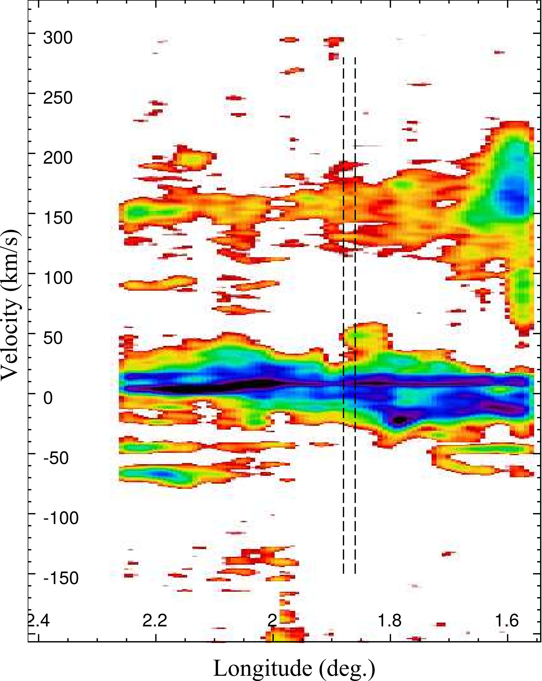
Figure 4 is a position-velocity image of Mopra CO(1-0) emission towards 0.9∘ of longitude encompassing G1.9+0.3. This image shows near-zero and 50 km s-1 components visible in the CO(1-0) spectrum (Figure 3), as well as gas at 150 km s-1 that can not be discerned in Figure 3. As noted by Roy & Pal 2014, gas at 150 km s-1 likely corresponds to the so-called ‘Feature-I’, which is close to the inner Galactic centre and extends to be background to Sgr A*. As noted earlier, this feature is seen in H i absorption by Roy & Pal 2014, but not confirmed in our analysis of ATCA H i data. We further note that a tentative H i emission component at 150 km s-1 may exist in Figure 3. However, since ‘Feature-I’ is very close to the Galactic Centre, a confirmation of this component would have little effect on the assumed G1.9+0.3 distance of 8.5 kpc.
| Image | R.M.S | 5 | Resolution | Synthesised |
|---|---|---|---|---|
| type | (mJy beam-1) | (mJy beam -1) | (km s-1) | Beam & P.A. |
| Continuum Map | 2.5 | 12.4 | N/A | 14.75′′ 5.86′′, 19.4° |
| Total Intensity Cube | 31.5 | 157.8 | 0.1 | 14.75′′ 5.86′′, 19.4° |
| Spectrum Cube | 3.5 | 17.5 | 1 | 14.75′′ 5.86′′, 19.4° |
3.2 Expansion
Given the lack of known young Galactic SNRs, confirmation of the age as well as the measurement of its expansion is very important for evolutionary studies. The calculation of G1.9+0.3 age and expansion rate follows the method described in De Horta et al. 2014 and Roper et al. 2018
Expansion is calculated across multiple radio-continuum images from between 1984 and 2017, produced from observations using both the VLA and ATCA. Details of the observations are in Table 4. These images were smoothed/convolved to a single beam size (matched to the lowest resolution image – 11.12′′ 5.32′′). They were then regridded to ensure that all images had the same center of RA(J2000)=17h48m45s and DEC(J2000)=–27∘10′6.7′′and same pixel size. Shell profiles were then measured over 32 arcs, beginning at due west and continuing counter-clockwise (paralactic angle, see Figure 6). 32 arcs were chosen to avoid over-sampling the images, giving a shell profile every 11∘ in SNR shell azimuth, demonstrated in Figure 7.
Using the shell profiles measured from all 8 epochs over a single arc, we measure the distance from the SNR centre to the peak radio brightness along the shell. These radii data points were plotted against corresponding years, and a least squares fit to the line was used to determine the expansion rate in arcseconds per unit of time. The residuals from the fitted line were used to establish the statistical uncertainty of this expansion rate. In this analysis, the southern break-out region where no clear shell profile could be discerned was excluded, demonstrated in Figure 7.
Once the entire SNR (at each given observation date) had been measured and fitted lines produced, we estimated the expansion of G1.9+0.3 (in arcseconds per year, percentage per year and kilometres per second), and finally, the approximate free-expansion age. The former is shown in Figures 5 and 6. The areas on Figure 6 marked with a horizontal green, purple, black and orange line and labelled “W”, “N-NE”, “E-SE” and “S” correspond to the areas introduced by Borkowski et al. 2017, demonstrated in Figure 7. This allows us to directly compare our radio continuum expansion study to the X-ray estimates. We have included in Table 5 the mean expansion rates and age, as well as the maximum expansion rates and age based thereupon. As expected, these are the regions with the largest expansion rate at both wavebands.
Overall, we have found that the SNR G1.9+0.3 has expanded between 1984 and 2017 at an average rate of (0.780.09) per cent per yr or (8 9001 200) km s-1 which implies a free-expansion age of (14219) yrs, dating this SNR explosion to mid-to-late 19th century. This result agrees with previous studies estimating an expansion rate of (0.6420.049) per cent per yr by Borkowski et al. 2017; Carlton et al. 2011 and is slightly faster than the (0.5630.078) per cent per yr measured by De Horta et al. 2014.
| Observing | Project | Telescope | Array Configuration | Bandwidth | Frequency | Original Synthesised | Original Position |
|---|---|---|---|---|---|---|---|
| Date | Code | Configuration | (MHz) | (GHz) | Beam | Angle | |
| 26/05/1984 | AG0146 | VLA | C | 50 | 4.8351 & 4.8851 | 7.76′′ 3.43′′ | –6.2° |
| 16/04/1985 | AG0184 | VLA | B | 50 | 1.4649 & 1.5149 | 2.78′′ 1.11′′ | –5.5° |
| 22/02/1987 | AB0407 | VLA | CD | 50 | 4.8351 & 4.8851 | 10.05′′ 9.27′′ | +64.1° |
| 23/06/1989 | AB0544 | VLA | BC | 50 | 4.8351 & 4.8851 | 8.03′′ 3.35′′ | –26.3° |
| 12/03/2008 | AG0793 | VLA | C | 50 | 4.8351 & 4.8851 | 2.78′′ 1.11′′ | –5.5° |
| 20/01/2009 | C1952 | ATCA | EW352 + 6C | 128 | 4.5440 & 5.1840 | 11.12′′ 5.32′′ | –0.8° |
| 19/02/2016 | C1952 | ATCA | EW352 + 6B | 4096 | 2.1000 & 5.0000 | 7.74′′ 3.51′′ | –5.5° |
| 20/05/2017 | C1952 | ATCA | 6A | 4096 | 2.1000 & 5.0000 | 1.80′′ 0.68′′ | +2.4° |
| Average | Maximum | Average | Maximum | Average | Maximum | Average | Minimum | |
|---|---|---|---|---|---|---|---|---|
| Region | Expansion | Expansion | Expansion | Expansion | Expansion | Expansion | Age | Age |
| (arcsec year-1) | (arcsec year-1) | (% year-1) | (% year-1) | (km s-1) | (km s-1) | (years) | (years) | |
| Overall | 0.22 0.03 | 0.34 0.08 | 0.78 0.09 | 1.20 0.23 | 8854 1195 | 13616 3075 | 142 19 | 93 7 |
| West | 0.18 0.03 | 0.19 0.04 | 0.65 0.09 | 0.67 0.11 | 7364 1248 | 7627 1462 | 155 18 | 149 15 |
| North | 0.18 0.03 | 0.21 0.05 | 0.56 0.10 | 0.65 0.16 | 7338 1290 | 8539 2059 | 178 18 | 153 11 |
| East | 0.28 0.03 | 0.34 0.08 | 0.84 0.10 | 1.02 0.23 | 11181 1324 | 13616 3075 | 119 17 | 98 7 |
| South | 0.23 0.01 | 0.24 0.02 | 0.90 0.04 | 0.96 0.06 | 9196 545 | 9798 731 | 111 41 | 104 31 |

3.3 Polarisation
The polarisation of a SNR can be an additional clue towards its age, with young SNR’s typically exhibiting a radially orientated magnetic field (Reynolds et al. 2012). At the same time, polarisation is an indicator of the emission mechanism of the SNR, with the presence of polarisation indicative of non-thermal emission from high energy electrons. As a shock evolves and sweeps-up an increasing mass, the shock is expected to decelerate, giving rise to Rayleigh–Taylor instabilities (Gull 1975; Chevalier 1976). As this occurs, the magnetic field lines become increasingly disordered and toroidal, which is apparent from the disordered polarisation vectors (Gull 1973; Johnston et al. 2004). This is largely borne out by similarly young Type Ia SNR’s (Milne 1987), as well as those in the LMC (Bozzetto et al. 2014, LMC;).
The ATCA, by default, records the Stokes Q and U parameters required to calculate the polarisation vectors. This ensures that as long as the secondary calibrator is observed regularly, and the data are correctly calibrated, then the resultant polarisation map will be reliable.
The full resolution polarisation images and the RM map have very little signal-to-noise ratio. For a better analysis we therefore convolved the Q and U maps in the four bands to a common resolution of 9′′. We re-calculated maps of polarised intensity (PI) and polarisation angle and the resulting RM at the resolution of 9′′. The resulting RM map and an integrated polarised intensity map across the whole band around 5 GHz are displayed in Figure 8-left. We also corrected the observed polarisation angles for Faraday rotation and added the corrected B-vectors to the PI map in Figure 8-right.
In the RM map in Figure 8-left we can see that the eastern (left) shell is dominated by high positive RM of about +400 to +600 rad m-2, while the western (right) shell shows mostly low positive RM of about 100 to 200 rad m-2. To quantify the distributions of RM on both of the shells we plot RM values as a function of Right Ascension (RA) in Figure 9. Dashed lines represent the mean values of the eastern and western shells, 411 rad m-2 and 123 rad m-2 respectively. The two concentrations of RM at about and just below belong to the weakly polarised northern part of the shell (see left panel in Figure 8). In Figure 8-right the derived magnetic field vectors in the southern parts of the shells seem to be mostly parallel to the shock normal (parallel from now on), with an average angle of about to the RA axis. To the north, the eastern shell shows a departure from the parallel magnetic field at a Declination of about exhibiting close to tangential field (perpendicular to the shock normal; perpendicular from now on). This change in the field structure also coincides with a region of elevated RM value. The parallel magnetic field seems to continue further north for the Western shell, but then changes towards the weakly polarised blobs in the northern part of the shell. This difference in intrinsic magnetic field directions projected to the plane of the sky might be caused by possible interaction of the SNR shell with molecular material in the north.

3.4 Spectral Index
We estimated the spectral index in Figure 10 by fitting a line to the 20 flux densities, integrated over the source, between 76.155 MHz and 227.195 MHz measured by the GLEAM project using the MWA (Hurley-Walker et al. 2017, MWA;), an 843 MHz flux density taken from Murphy et al. 2008 measured with the MOST and scaled by 12 per cent to account for the brightening found within their paper, and the flux densities measured from our 2016 ATCA observations. Our flux densities were measured from the 2016 ATCA 2.1, 5 and 9 GHz images, where they had all been convolved to the same beam and pixel size. The 2.1 GHz image was then masked to 20 ( 0.16 mJy beam-1) and then used to mask the 5 and 9 GHz images to ensure the flux density measurements were taking into account the same pixels for all images. All flux densities used in Figure 10 are listed in Table 6.
Using these flux densities, we obtain a spectral index of 0.02 — shown in Figure 10 — which is comparable to the spectral index of –0.93 0.23 calculated by LaRosa et al. 2000. However, it is steeper than the spectral index calculated by Green et al. 2008 of –0.620.06. Green et al. 2008 note that their estimated spectral index differs from values in the literature, and instead suggest a spectral index of –0.7, which is closer to the spectral index estimated here. With a spectral index of –0.81 0.02, G1.9+0.3 has one of the steepest spectral indexes known in our Galaxy and MCs (Bozzetto et al. 2017; Maggi et al. 2019, MCs; ).
Such a steep spectral index is characteristic of young SNR (Urošević 2014). The steep spectra of young SNRs can be caused by quasi-perpendicular magnetic field geometry (Bell et al. 2011), turbulent magnetic field amplification (Bell et al. 2019), Alfvenic drift effect (Jiang et al. 2013), and by pure NLDSA effects which efficiently produce strong magnetic field amplification (Pavlović 2017).
By using the radio spectrum from the ATCA, MOST and MWA (MWA) in conjunction with the distance of 8.5 kpc and a diameter of 95′′, we can calculate the total flux density at 1 GHz (0.99 Jy) surface Brightness ( W (m2 Hz SR)-1) and luminosity between 10 MHz and 100 GHz (0.891026 W Hz-1).
The spectral index map presented in Figure 11 is the product of the miriad task mfspin, with our 2.1, 5.0 and 9.0 GHz data combined into a single uv file before imaging, with the uv range tapered to ensure matching coverage across all bands. This image was then masked to 20 – where is measured to be 0.05 mJy beam-1, before the miriad task mfspin was run, allowing for the final 20 spectral index map in Figure 11 to be created. The steepest section of this spectral index map is measured at –1.07 in the northern region, where we also see somewhat randomised polarisation vectors (Figure 8) and extreme radio brightening in Section 3.5. The average spectral index measured across the SNR is –0.61, with a standard deviation of 0.18.
We would not necessarily expect the spectral index presented in Figure 10 to be equivalent to the average spectral index measured from the spectral index map presented in Figure 11, as the spectral index presented in Figure 10 is effectively taking the average across the map unweighted by flux density, whereas the spectral index map in Figure 11 is effectively weighted by the flux density.
| Instrument | (MHz) | (Jy) |
|---|---|---|
| MWA | 76.155 | 8.438 |
| MWA | 83.835 | 8.022 |
| MWA | 91.515 | 7.216 |
| MWA | 99.195 | 6.734 |
| MWA | 106.875 | 7.184 |
| MWA | 114.555 | 5.827 |
| MWA | 122.235 | 5.953 |
| MWA | 129.915 | 5.135 |
| MWA | 142.715 | 5.885 |
| MWA | 150.395 | 4.512 |
| MWA | 158.075 | 4.556 |
| MWA | 165.755 | 3.261 |
| MWA | 173.435 | 3.838 |
| MWA | 181.115 | 4.301 |
| MWA | 188.795 | 4.240 |
| MWA | 196.475 | 3.575 |
| MWA | 204.155 | 3.263 |
| MWA | 211.835 | 3.044 |
| MWA | 219.515 | 3.518 |
| MWA | 227.195 | 2.188 |
| MOST | 843.000 | 1.104 |
| ATCA | 2100.000 | 0.645 |
| ATCA | 5000.000 | 0.249 |
| ATCA | 9000.000 | 0.181 |


3.5 Radio Brightening
In Figure 12, a striking difference in the northern shock position was observed, with the 2017 G1.9+0.3 image extending farther north than 2016 image. By taking our 2.1 GHz observations from March 2016 with the ATCA in a 6B configuration and our 2.1 GHz observations from May 2017 with the ATCA in a 6A configuration imaged to the same beam size, we can construct an image comparing the flux density levels from each. Figure 13 is an image that shows the relative radio flux density brightening, calculated using Equation 1 across the 14 month period.
| (1) |
We mask the resulting image so that any pixel is masked if it is below 10 in either the 2016 image (0.16 mJy beam-1, or in the 2017 image (0.28 mJy beam-1).
The brightness percentage map in Figure 13 has an average increase of 1.95 per cent. There is a minimum of –57.08 per cent, and a maximum brightening of 228.30 per cent along the northern region where we found decreased expansion in Section 3.2, a less-ordered polarisation field as can be seen in Figure 8-Right and a steep spectral index in Section 3.4.
By interpolating this 1.95 per cent brightening rate from the measured 14 months to 12 months, we find an average brightening of (1.670.35) per cent per yr (consistent with the value of 1.8 per cent predicted by simulations in Pavlović 2017), minimum brightening rate of –50 per cent per yr and a maximum brightening rate of 200 per cent per yr. Our new average result is in line with the (1.22) per cent per yr measured by Murphy et al. 2008 with their study over 20 years using the MOST, and the 2 per cent increase per year measured by Green et al. 2008 with the VLA.


4 Discussion
SNR G1.9+0.3 is unique, in that it is the youngest known Galactic Type Ia SNR. As such, it provides a window into the evolution of the young SNR. While some of the observations demonstrated are within the expected and currently measured bounds – Radio expansion rate and spectral index – some observations differ.
The RM map shown in Figure 9 is indicative of one of the divergences from current observations. A similar behaviour for the distribution of RM on the two opposite shells of an SNR were found for the SNR G296.5+10.0 by Harvey-Smith et al. 2010. They found relatively constant RM of opposite sign on both shells of the SNR. As G1.9+0.3 is estimated to be further away, and closer to the centre of our Galaxy, we would expect quite significant foreground RM. Assuming a positive foreground RM of about +267 rad m-2, the internal eastern and western shell RM would be roughly matched with opposite signs of about rad m-2 (see Figure 9). We tried to analyse the foreground RM by comparing RM of pulsars and extra-galactic sources, at short angular distances from the SNR. For the pulsars we are using the “The Australia Telescope National Facility Pulsar Catalogue” (Manchester et al. 2005)22 2 http://www.atnf.csiro.au/research/pulsar/psrcat/. We find two pulsars with known RM of +421 and +916 rad m-2 within of G1.9+0.3 (Han et al. 2018) with DM (DM) distances of 5.2 and 4.2 kpc, respectively (Yao et al. 2017). There are two linearly polarised background extra-galactic sources with RM of +806 and +638 rad m-2 within of G1.9+0.3 taken from a catalog of Faraday RM of point sources published by Xu & Han 201433 3 http://zmtt.bao.ac.cn/RM/searchGRM.html. These values indicate that the RM in this direction are varying a lot and are in general positive with a high amplitude. A foreground RM of +267 rad m-2 is certainly not unexpected, but is low compared to other RM from the same direction. However, it also cannot be excluded that the difference in the RM between the eastern and western shell is simply due to variations of the foreground RM.
Harvey-Smith et al. 2010 showed that such a behaviour of the RM in G296.5+10.0 can be explained by a SNR expanding inside an azimuthal/toroidal magnetic field in the stellar wind of the progenitor star of the SN explosion. In this case, magnetic field lines would be wrapped around the expanding SNR in the equatorial region which in the projected picture will show up as a quasi-radial field inside the shell with the decrease of the in-plane component towards the edge of the remnant. This roughly corresponds to what we see in G1.9+0.3 (see Figure 8-left) if the equatorial plane is tilted by with respect to the RA axis. From such a magnetic field configuration we would expect the RM to have the same amplitude on both shells but opposite sign. Harvey-Smith et al. 2010 simulated the expansion of a late time stellar wind of the progenitor star in order to calculate the RM that would be imposed on background linearly polarised emission. They studied several different progenitor stars and showed that the RSG (RSG) wind can be responsible for the levels of the RM in G296.5+10.0. Using the same formalism, it is easy to demonstrate that this could also be a plausible scenario to explain the RM distribution in G1.9+0.3.
However, the RSG wind and toroidal magnetic field hypothesis does not explain all aspects of this SNR.
First, to reach the size of G1.9+0.3 in this scenario, the age of the SNR would need to be closer to 400 years old (Dwarkadas 2005; Telezhinsky et al. 2013), because of the expected shock speed of a SNR expanding inside the stellar wind of the progenitor star. A super-luminous SN explosion would be required to reach the expansion velocity and size observed in G1.9+0.3. Additionally, the lower shock speed anticipated from this scenario would result in a lower maximum electron energy, which would be difficult to reconcile with the observed X-ray emission. The RSG-scenario should produce more thermal X-ray emission than reported by Borkowski et al. 2013.
Second, the RSG-scenario would make G1.9+0.3 a twin of Cassiopeia A, which would raise the question – why are the respective morphologies so different?
Third, a toroidal magnetic field in the stellar wind of the progenitor star would be parallel to the shock, which makes particle acceleration at the shock very inefficient (Caprioli & Spitkovsky 2014; Völk et al. 2003) which in turn results in a lack of magnetic field amplification by the CR. This contradicts the explanation of the synchrotron emission from the SNR. Theoretical modeling requires a high magnetic field downstream of the forward shock with estimates ranging from 180 G (Brose et al. 2019) to G (Pavlović 2017; Urošević et al. 2018) which in turn are in agreement with an equipartition magnetic field of G (De Horta et al. 2014).
Finally, simulations presented in Brose et al. 2019 strongly suggest that radio emission predominantly originates from the reverse shock, which means that it is not sensitive to the the structure of the magnetic field upstream of the forward shock. A dedicated study of polarisation of the X-ray emission would be extremely important to solve some of these discrepancies.
Unexpected radio brightening was also observed in the northern region. Uchiyama et al. 2007 has previously observed localised brightening (and fading; explained by synchrotron cooling) of X-ray emission in RX J1713.73946 on a one year timescale. This was said to be synchrotron emission from electrons quickly accelerated by the diffusive shock acceleration (DSA) process, and the high energy of the variable emission indicated magnetic field amplification in that region of the SNR shock, which corresponds to dense molecular clumps (Sano et al. 2010; Maxted et al. 2013; Sano et al. 2015). Therefore, the largest brightening increase in the northern parts of G1.9+0.3 (Figure 13) may indicate regions of shock interaction with a highly inhomogeneous ISM. This motivates future X-ray studies probing small-scale X-ray features as well as future ISM observations at arc-sec resolution (e.g. using ALMA, e.g. see Sano et al. 2019, or ATCA) to identify shock/ISM interactions.
In addition to exhibiting short-timescale X-ray brightening linked to particle acceleration, SNR RX J1713.7-3946 is a strong TeV gamma-ray source (Aharonian et al. 2007; H.E.S.S. Collaboration et al. 2018) and has been the subject of a number of investigations that search for signatures of CR hadrons accelerated within the SNR shell (Fukui et al. 2012, e.g.). The localised radio brightening of G1.9+0.3 discovered in our study highlights the potential of G1.9+0.3 as a powerful particle accelerator as well. Indeed, as argued in Section 3.3, the B-field amplification implied by strong synchrotron X-ray emission can be naturally explained by CRs (e.g. CR streaming instabilities). It follows that this object is a key target in CR origin studies with future high-sensitivity TeV gamma-ray observations of the Cherenkov Telescope Array (Cherenkov Telescope Array Consortium et al. 2019, CTA, see).
5 Conclusion
This radio study of the youngest known Galactic SNR has used new ATCA observations in 2016 and 2017 and preliminary observations from the Mopra and MWA telescopes to examine the flux density, distance, spectral index, polarisation, brightening and expansion of the G1.9+0.3 shell. Our main findings are:
- •
Our H i and CO study is consistent with a distance of 8.5 kpc;
- •
G1.9+0.3 has a mean expansion (in radio continuum) rate of (0.78 0.09) per cent per yr over a 31 year period, equivalent to (88001200) km s-1 at a distance of 8.5 kpc;
- •
There are very different RM values towards the two so called (east & west) “ears” of G1.9+0.3. The expansion into the stellar wind of a RGS star progenitor could potentially explain the polarisation characteristics we observe for SNR G1.9+0.3. This hypothesis, however, would have difficulties explaining hydrodynamic properties of the remnant and its observed X-ray emission;
- •
G1.9+0.3 has a global spectral index of (-0.81 0.02), which steepens to towards the remnant’s north, where we also find increased brightening of up to 195 per cent, consistent with brightening due to expansion into an inhomogeneous ISM;
- •
There is an average radio brightening of (1.67 0.35) per cent per yr;
Acknowledgements
The ATCA is part of the Australia Telescope National Facility which is funded by the Commonwealth of Australia for operation as a National Facility managed by CSIRO (CSIRO). This paper includes archived data obtained through the Australia Telescope Online Archive (http://atoa.atnf.csiro.au). We used the karma and miriad software packages developed by the ATNF (ATNF) and the python programming language. This work is part of the project 176005 “Emission nebulae: structure and evolution” supported by the Ministry of Education, Science, and Technological Development of the Republic of Serbia.
References
- Aharonian et al. (2007) Aharonian F., et al., 2007, A&A, 464, 235
- Bell et al. (2011) Bell A. R., Schure K. M., Reville B., 2011, MNRAS, 418, 1208
- Bell et al. (2019) Bell A. R., Matthews J. H., Blundell K. M., 2019, MNRAS, 488, 2466
- Blackwell et al. (2019) Blackwell R., et al., 2019, Publ. Astron. Soc. Australia, submitted
- Borkowski et al. (2010) Borkowski K. J., Reynolds S. P., Green D. A., Hwang U., Petre R., Krishnamurthy K., Willett R., 2010, ApJ, 724, L161
- Borkowski et al. (2013) Borkowski K. J., Reynolds S. P., Hwang U., Green D. A., Petre R., Krishnamurthy K., Willett R., 2013, ApJ, 771, L9
- Borkowski et al. (2017) Borkowski K. J., Gwynne P., Reynolds S. P., Green D. A., Hwang U., Petre R., Willett R., 2017, ApJ, 837, L7
- Bozzetto et al. (2014) Bozzetto L. M., Filipović M. D., Urošević D., Kothes R., Crawford E. J., 2014, MNRAS, 440, 3220
- Bozzetto et al. (2017) Bozzetto L. M., et al., 2017, ApJS, 230, 2
- Braiding et al. (2018) Braiding C., et al., 2018, Publ. Astron. Soc. Australia, 35, e029
- Brose et al. (2019) Brose R., Sushch I., Pohl M., Luken K. J., Filipovic M. D., Lin R., 2019, arXiv e-prints, p. arXiv:1906.02725
- Burton et al. (2013) Burton M. G., et al., 2013, Publ. Astron. Soc. Australia, 30, e044
- Cappellaro et al. (2005) Cappellaro E., Barbon R., Turatto M., 2005, in Marcaide J.-M., Weiler K. W., eds, Vol. 99, IAU Colloq. 192: Cosmic Explosions, On the 10th Anniversary of SN1993J. p. 347, doi:10.1007/3-540-26633-X_48
- Caprioli & Spitkovsky (2014) Caprioli D., Spitkovsky A., 2014, ApJ, 783, 91
- Carlton et al. (2011) Carlton A. K., Borkowski K. J., Reynolds S. P., Hwang U., Petre R., Green D. A., Krishnamurthy K., Willett R., 2011, ApJ, 737, L22
- Cherenkov Telescope Array Consortium et al. (2019) Cherenkov Telescope Array Consortium et al., 2019, Science with the Cherenkov Telescope Array. World Scientific Publishing Co, doi:10.1142/10986
- Chevalier (1976) Chevalier R. A., 1976, ApJ, 207, 872
- Cohen (1975) Cohen R. J., 1975, MNRAS, 171, 659
- De Horta et al. (2014) De Horta A. Y., et al., 2014, Serbian Astronomical Journal, 189, 41
- Dwarkadas (2005) Dwarkadas V. V., 2005, ApJ, 630, 892
- Farnes (2012) Farnes J. S., 2012, PhD thesis, University of Cambridge j.farnes@mrao.cam.ac.uk
- Francis & Anderson (2014) Francis C., Anderson E., 2014, MNRAS, 441, 1105
- Fukui et al. (2012) Fukui Y., et al., 2012, ApJ, 746, 82
- Gómez & Rodríguez (2009) Gómez Y., Rodríguez L. F., 2009, Rev. Mex. Astron. Astrofis., 45, 91
- Gooch (2011) Gooch R., 2011, Karma: Visualisation Test-Bed Toolkit, Astrophysics Source Code Library (ascl:1102.018)
- Gray (1994) Gray A. D., 1994, MNRAS, 270, 847
- Green & Gull (1984) Green D. A., Gull S. F., 1984, Nature, 312, 527
- Green et al. (2008) Green D. A., Reynolds S. P., Borkowski K. J., Hwang U., Harrus I., Petre R., 2008, MNRAS, 387, L54
- Gull (1973) Gull S. F., 1973, MNRAS, 161, 47
- Gull (1975) Gull S. F., 1975, MNRAS, 171, 263
- H.E.S.S. Collaboration et al. (2018) H.E.S.S. Collaboration et al., 2018, A&A, 612, A6
- Han et al. (2018) Han J. L., Manchester R. N., van Straten W., Demorest P., 2018, ApJS, 234, 11
- Harvey-Smith et al. (2010) Harvey-Smith L., Gaensler B. M., Kothes R., Townsend R., Heald G. H., Ng C.-Y., Green A. J., 2010, ApJ, 712, 1157
- Hunter (2007) Hunter J. D., 2007, Computing In Science & Engineering, 9, 90
- Hurley-Walker et al. (2017) Hurley-Walker N., et al., 2017, MNRAS, 464, 1146
- Jiang et al. (2013) Jiang Z. J., Zhang L., Fang J., 2013, MNRAS, 433, 1271
- Johnston et al. (2004) Johnston S., McClure-Griffiths N. M., Koribalski B., 2004, MNRAS, 348, L19
- Kerr & Lynden-Bell (1986) Kerr F. J., Lynden-Bell D., 1986, MNRAS, 221, 1023
- LaRosa et al. (2000) LaRosa T. N., Kassim N. E., Lazio T. J. W., Hyman S. D., 2000, AJ, 119, 207
- Maggi et al. (2019) Maggi P., et al., 2019, arXiv e-prints, p. arXiv:1908.11234
- Manchester et al. (2005) Manchester R. N., Hobbs G. B., Teoh A., Hobbs M., 2005, AJ, 129, 1993
- Maxted et al. (2013) Maxted N., et al., 2013, Publ. Astron. Soc. Australia, 30, e055
- Milne (1987) Milne D. K., 1987, Australian Journal of Physics, 40, 771
- Murphy et al. (2008) Murphy T., Gaensler B. M., Chatterjee S., 2008, MNRAS, 389, L23
- Nord et al. (2004) Nord M. E., Lazio T. J. W., Kassim N. E., Hyman S. D., LaRosa T. N., Brogan C. L., Duric N., 2004, AJ, 128, 1646
- Pavlović (2017) Pavlović M. Z., 2017, MNRAS, 468, 1616
- Reynolds et al. (2008) Reynolds S. P., Borkowski K. J., Green D. A., Hwang U., Harrus I., Petre R., 2008, ApJ, 680, L41
- Reynolds et al. (2009) Reynolds S. P., Borkowski K. J., Green D. A., Hwang U., Harrus I., Petre R., 2009, ApJ, 695, L149
- Reynolds et al. (2012) Reynolds S. P., Gaensler B. M., Bocchino F., 2012, Space Sci. Rev., 166, 231
- Roper et al. (2018) Roper Q., et al., 2018, MNRAS, 479, 1800
- Roy & Pal (2014) Roy S., Pal S., 2014, in Ray A., McCray R. A., eds, IAU Symposium Vol. 296, Supernova Environmental Impacts. pp 197–201, doi:10.1017/S1743921313009460
- Sano et al. (2010) Sano H., et al., 2010, ApJ, 724, 59
- Sano et al. (2015) Sano H., et al., 2015, ApJ, 799, 175
- Sano et al. (2019) Sano H., et al., 2019, ApJ, 873, 40
- Sault et al. (1995) Sault R. J., Teuben P. J., Wright M. C., 1995, in Astronomical Data Analysis Software and Systems IV. p. 433
- Telezhinsky et al. (2013) Telezhinsky I., Dwarkadas V. V., Pohl M., 2013, A&A, 552, A102
- Uchiyama et al. (2007) Uchiyama Y., Aharonian F. A., Tanaka T., Takahashi T., Maeda Y., 2007, Nature, 449, 576
- Urošević (2014) Urošević D., 2014, Ap&SS, 354, 541
- Urošević et al. (2018) Urošević D., Pavlović M. Z., Arbutina B., 2018, ApJ, 855, 59
- Völk et al. (2003) Völk H. J., Berezhko E. G., Ksenofontov L. T., 2003, A&A, 409, 563
- Wayth et al. (2015) Wayth R. B., et al., 2015, Publ. Astron. Soc. Australia, 32, e025
- Wilson et al. (2011) Wilson W. E., et al., 2011, MNRAS, 416, 832
- Xu & Han (2014) Xu J., Han J.-L., 2014, Research in Astronomy and Astrophysics, 14, 942
- Yao et al. (2017) Yao J. M., Manchester R. N., Wang N., 2017, ApJ, 835, 29
- de Grijs & Bono (2016) de Grijs R., Bono G., 2016, ApJS, 227, 5
- van den Bergh & Tammann (1991) van den Bergh S., Tammann G. A., 1991, ARA&A, 29, 363