Black holes with a nonconstant kinetic term in degenerate higher-order scalar tensor theories

Masato Minamitsuji Affiliation: Centro de Astrofísica e Gravitação - CENTRA, Departamento de Física, Instituto Superior Técnico - IST, Universidade de Lisboa - UL, Av. Rovisco Pais 1, 1049-001 Lisboa, Portugal James Edholm Affiliation: Physics Department, Lancaster University, Lancaster, LA1 4YW

Abstract

We investigate static and spherically symmetric black hole (BH) solutions in shift-symmetric quadratic-order degenerate higher-order scalar-tensor (DHOST) theories. We allow a nonconstant kinetic term $X=g^{\mu\nu}\partial_{\mu}\phi\partial_{\nu}\phi$ for the scalar field $\phi$ and assume that $\phi$ is, like the spacetime, a pure function of the radial coordinate $r$ , namely $\phi=\phi(r)$ . First, we find analytic static and spherically symmetric vacuum solutions in the so-called Class Ia DHOST theories, which include the quartic Horndeski theories as a subclass. We consider several explicit models in this class and apply our scheme to find the exact vacuum BH solutions. BH solutions obtained in our analysis are neither Schwarzschild or Schwarzschild (anti-) de Sitter. We show that a part of the BH solutions obtained in our analysis are free of ghost and Laplacian instabilities and are also mode stable against the odd-parity perturbations. Finally, we argue the case that the scalar field has a linear time dependence $\phi=qt+\psi(r)$ and show several simple examples of nontrivial BH solutions with a nonconstant kinetic term obtained analytically and numerically.

I Introduction

Scalar-tensor theories have provided the unified mathematical description of modified gravity theories Berti et al. 2015. In classic scalar-tensor theories, whose Lagrangian density depends on the metric $g_{\mu\nu}$ , the scalar field $\phi$ , and its first-order derivative $\phi_{\mu}:=\nabla_{\mu}\phi$ , ${\cal L}={\cal L}(g_{\mu\nu},\phi,\phi_{\mu})$ , the Euler-Lagrange (EL) equations are given by the second-order differential equations. However, the Lagrangian density of modern scalar-tensor theories may also contain the second-order derivatives of the scalar field $\phi_{\mu\nu}:=\nabla_{\mu}\nabla_{\nu}\phi$ . Although generically the EL equations in such theories contain higher derivative terms, the appearance of Ostrogradsky ghosts Woodard 2015 can be avoided using certain degeneracy conditions Motohashi et al. 2016a. Degenerate higher-order scalar-tensor (DHOST) theories Langlois and Noui 2016; Crisostomi et al. 2016; Ben Achour et al. 2016a; Ben Achour et al. 2016b; Crisostomi and Koyama 2018; Langlois et al. 2018 (see also Langlois 2019; Kobayashi 2019) provide the most general framework of scalar-tensor theories which are free from Ostrogradsky instabilities Woodard 2015, and hence the system contains only three degrees of freedom (DOFs), namely, two tensorial and one scalar polarizations (See § II for details). Applications of DHOST theories to cosmological and astrophysical problems have been investigated in Refs. Langlois et al. 2017; Langlois et al. 2018; Dima and Vernizzi 2018; Creminelli et al. 2018; Saltas and Lopes 2019.

The application of modern scalar-tensor theories to BH physics has attracted great interest. Besides the Schwarzschild or Kerr solutions in General Relativity (GR) with or without a constant scalar field Motohashi and Minamitsuji 2018; Motohashi and Minamitsuji 2019, i.e. GR BH solutions, they also allow BH solutions which are absent in GR. A typical nontrivial BH solution is the stealth Schwarzschild solution Babichev and Charmousis 2014; Kobayashi and Tanahashi 2014 obtained in shift-symmetric Horndeski theories with the assumptions of a linearly time-dependent scalar field $\phi=qt+\psi(r)$ and a constant kinetic term $X={\rm const}$ , where $t$ and $r$ are the time and radial coordinates of the static and spherically symmetric spacetime and $X:=g^{\mu\nu}\phi_{\mu}\phi_{\nu}$ represents the canonical kinetic term of the scalar field. In stealth solutions, the spacetime geometry is completely independent of the coupling functions and the profiles of the scalar field. Stealth Schwarzschild solutions have also been found in shift-symmetric DHOST theories in Refs. Ben Achour and Liu 2019; Motohashi and Minamitsuji 2019; Takahashi et al. 2019; Minamitsuji and Edholm 2019. Another nontrivial solution is the Schwarzschild-(anti-) de Sitter solution with the same properties of the scalar field Babichev and Charmousis 2014; Kobayashi and Tanahashi 2014; Babichev et al. 2018; Ben Achour and Liu 2019; Motohashi and Minamitsuji 2019; Takahashi et al. 2019; Minamitsuji and Edholm 2019. Kerr-(anti-) de Sitter solutions with a constant $X$ were obtained in Ref. Charmousis et al. 2019a; Charmousis et al. 2019b. It was recently argued, however, that stealth or Schwarzschild-(anti-) de Sitter BH solutions with the constant kinetic term suffer issues of the strong coupling in the sector of the scalar perturbations de Rham and Zhang 2019. Neutron star (NS) solutions were also explicitly constructed in Ref. Kobayashi and Hiramatsu 2018. In this paper, we will investigate BH solutions with a nonconstant $X$ in quadratic DHOST theories.

While BH solutions with a constant $X$ can be obtained without explicitly specifying the functions which determine the coupling of the scalar field, those with a nonconstant $X$ will require explicit choices of these coupling functions. Static and spherically symmetric BH solutions obtained without the assumption of a nonconstant kinetic term typically have the metrics of neither Schwarzschild- nor Schwarzschild-(anti-) de Sitter spacetimes. In the context of the shift-symmetric Horndeski theory, the first exact static and spherically symmetric solutions with $\phi=\phi(r)$ and a nonconstant $X$ were asymptotically locally anti-de Sitter Rinaldi 2012; Anabalon et al. 2014; Minamitsuji 2014. An asymptotically flat solution with the static scalar field $\phi=\phi(r)$ was also constructed in a class of the shift-symmetric Horndeski theory with a linear coupling to the Gauss-Bonnet term Sotiriou and Zhou 2014a; Sotiriou and Zhou 2014b. However, in these solutions the Noether current $J^{\mu}$ does not vanish at the event horizon and the norm $J_{\mu}J^{\mu}$ blows up there Babichev et al. 2017. The static, spherically symmetric, and asymptotically flat BH solutions with both the ansatz of the scalar field $\phi=\phi(r)$ and $\phi=qt+\psi(r)$ , which were different from the Schwarzschild solution, were obtained in the shift-symmetric Horndeski and GLPV theories with vanishing Noether current $J^{\mu}=0$ under the assumption that $X$ is a nontrivial function of $r$ Babichev et al. 2017.

Recently, in Ref. Ben Achour et al. 2019 static and spherically symmetric BH solutions with a nonconstant $X=X(r)$ in the quadratic DHOST theories have been explored by the disformal transformation of the known BH solutions. In this paper, instead, we will focus on analytic BH solutions with a nonconstant $X$ by the direct integration of the equations of motion. Our approach will follow that developed in previous work to solve the problems in static and spherically symmetric systems Kobayashi and Hiramatsu 2018; Takahashi et al. 2019. Although the equations of motion are given by higher-order differential equations with respect to the radial coordinate $r$ , because of the properties of the underlying theories, these higher-order differential equations are degenerate and their combination provides a constraint relation. With this constraint relation, the system can reduce to that of the second-order differential equations.

The paper is constructed as follows: In § II, we give an overview of the quadratic DHOST theories. In § III, we present the strategy to find the static and spherically symmetric vacuum solutions with the scalar field $\phi=\phi(r)$ in the shift-symmetric Class Ia quadratic DHOST theories. In § IV, we present the explicit models and BH solutions with a nonconstant $X$ , and investigate the odd-mode stability of these solutions. In § V, we argue the case of a linearly time dependent scalar field $\phi=qt+\psi(r)$ , and provide several models giving rise to notrivial BH solutions analytically and numerically. The last § VI is devoted to a brief summary and conclusion.

II The DHOST Theories

In the context of analytical mechanics, a simple example of degenerate higher-derivative system is given by Langlois and Noui 2016; Langlois 2019; Kobayashi 2019

\displaystyle L=\frac{a_{1}}{2}\ddot{x}^{2}+a_{2}\ddot{x}\dot{y}+\frac{a_{3}}{2}\dot{y}^{2}+\frac{1}{2}\dot{x}^{2}+\cdots,

(1)

where ‘dot’ means a derivative with respect to time; the variables $x$ and $y$ are the straightforward analogs of the scalar field $\phi$ and the metric $g_{\mu\nu}$ in the scalar-tensor theories, respectively; $a_{i}$ ( $i=1,2,3$ ) are assumed to be constant for simplicity. The EL equations for $x$ and $y$ are given by $a_{1}\ddddot{x}+a_{2}\dddot{y}+\cdots=0$ and $a_{2}\dddot{x}+a_{3}\ddot{y}+\cdots=0$ , where dots denote the terms composed of the lower-order derivatives. Eliminating $y$ with the new variable $z=a_{2}\dot{x}+a_{3}y$ , we obtain the two independent equations $\left(a_{2}^{2}-a_{1}a_{3}\right)\ddddot{x}+\left(\cdots\right)\ddot{x}+\cdots=0$ and $\ddot{z}+\cdots=0$ . Generically, in order to determine evolution of the system, we need the six initial data of $x$ , $\dot{x}$ , $\ddot{x}$ , $\dddot{x}$ , $z$ , and $\dot{z}$ and hence there are 2 $+$ 1 DOFs, where the extra one is known as an Ostrogradsky ghost Woodard 2015. However, by imposing the additional condition $a_{2}^{2}-a_{1}a_{3}=0$ , the system reduces to that of the two second-order differential equations $\ddot{x}+\cdots=0$ and $\ddot{z}+\cdots=0$ , and contains 2 physical DOFs, namely, the Ostrogradsky ghost is eliminated. The condition like $a_{2}^{2}-a_{1}a_{3}=0$ is called the degeneracy condition. A degenerate theory corresponds to a class of higher-derivative theories where the EL equations can reduce to the second-order systems after a suitable redefinition of variables Langlois and Noui 2016; Motohashi et al. 2016a; Klein and Roest 2016; Motohashi et al. 2018a; Motohashi et al. 2018b.

DHOST theories correspond to the extension of the degenerate theories in analytical mechanics to scalar-tensor theories Langlois and Noui 2016; Ben Achour et al. 2016a; Ben Achour et al. 2016b; Crisostomi and Koyama 2018; Langlois et al. 2018. The construction of DHOST theories starts from the the most general covariant scalar-tensor Lagrangian density which contains up to second-order covariant derivatives of the scalar field $\phi_{\mu\nu}$ , ${\cal L}={\cal L}\left(g_{\mu\nu},\phi,\phi_{\mu},\phi_{\mu\nu}\right)$ , and then expands it in terms of $\phi_{\mu\nu}$ as

\displaystyle\frac{{\cal L}}{\sqrt{-g}}

\displaystyle=

\displaystyle F_{0}(\phi,X)-F_{1}(\phi,X)\Box\phi+F_{2}(\phi,X)R+F_{3}(\phi,X)G^{\alpha\beta}\phi_{\alpha\beta}+C_{2}^{\alpha\beta\rho\sigma}\left(g_{\mu\nu},\phi,\phi_{\mu}\right)\phi_{\alpha\beta}\phi_{\rho\sigma}+{\cal O}\left[(\phi_{\rho\sigma})^{3}\right],

(2)

where $R$ and $G^{\alpha\beta}$ are the Ricci scalar and Einstein tensor associated with the metric $g_{\mu\nu}$ ; $\phi_{\mu\nu\cdots\alpha}:=\nabla_{\mu}\nabla_{\nu}\cdots\nabla_{\alpha}\phi$ represents the covariant derivative associated with $g_{\mu\nu}$ ; $X=g^{\mu\nu}\phi_{\mu}\phi_{\nu}$ is the ordinary kinetic term; $\Box\phi:=g^{\mu\nu}\phi_{\mu\nu}$ ; and $C_{2}^{\alpha\beta\rho\sigma}$ is a general rank-4 covariant tensor constructed from $g_{\mu\nu}$ , $\phi$ and $\phi_{\mu}$ with certain symmetries. We note that in the above theory (2) the $F_{0}$ and $F_{1}$ terms correspond to a part of the Horndeski theory Horndeski 1974; Deffayet et al. 2009a; Deffayet et al. 2009b; Deffayet et al. 2011; Kobayashi et al. 2011. Truncating Eq. (2) at the order of $\phi_{\mu\nu}^{2}$ and setting $F_{1}=F_{3}=0$ ^*1^*1 *1 We set $F_{1}=F_{3}=0$ , as we will focus on the shift- and reflection-symmetric theories., we obtain

\displaystyle\frac{{\cal L}}{\sqrt{-g}}=F_{0}(\phi,X)+F_{2}(\phi,X)R+\sum_{I=1}^{5}A_{I}(\phi,X)L_{I}^{(2)},

(3)

where

\displaystyle L_{1}^{(2)}=\phi_{\mu\nu}\phi^{\mu\nu},\quad L_{2}^{(2)}=\left(\Box\phi\right)^{2},\quad L_{3}^{(2)}=\Box\phi\phi^{\mu}\phi_{\mu\nu}\phi^{\nu},\quad L_{4}^{(2)}=\phi^{\mu}\phi_{\mu\rho}\phi^{\rho\nu}\phi_{\nu},\quad L_{5}^{(2)}=\left(\phi_{\mu}\phi^{\mu\nu}\phi_{\nu}\right)^{2},

(4)

where $A_{I}(\phi,X)$ ( $I=1,\cdots,5$ ) are functions of $\phi$ and $X$ . Degeneracy conditions for the quadratic DHOST theory (3) were obtained in Refs Langlois and Noui 2016; Ben Achour et al. 2016a; Ben Achour et al. 2016b. Among them, we focus on the Class Ia (also known as Class ²N-I) DHOST theories Langlois and Noui 2016; Ben Achour et al. 2016a for which the degenerate conditions are given by

$\displaystyle A_{2}$	$\displaystyle=$	$\displaystyle-A_{1}\neq-\frac{F_{2}}{X},$
$\displaystyle A_{4}$	$\displaystyle=$	$\displaystyle\frac{1}{8(F_{2}-XA_{1})^{2}}\left\{4F_{2}\left[3(A_{1}-2F_{2X})^{2}-2A_{3}F_{2}\right]-A_{3}X^{2}(16A_{1}F_{2X}+A_{3}F_{2})\right.$
		$\displaystyle\left.+4X\left[3A_{1}A_{3}F_{2}+16A_{1}^{2}F_{2X}-16A_{1}F_{2X}^{2}-4A_{1}^{3}+2A_{3}F_{2}F_{2X}\right]\right\},$
$\displaystyle A_{5}$	$\displaystyle=$	$\displaystyle\frac{1}{8(F_{2}-XA_{1})^{2}}(2A_{1}-XA_{3}-4F_{2X})\left(A_{1}(2A_{1}+3XA_{3}-4F_{2X})-4A_{3}F_{2}\right).$	(5)

The theory (3) with Eq. (II) includes the quintic-order Horndeski Horndeski 1974 and Gleyzes-Langlois-Piazza-Vernizzi (GLPV) Gleyzes et al. 2015 theories as subclasses. The other classes of the quadratic DHOST theories suffer Laplacian instabilities of scalar perturbations in cosmological backgrounds Langlois et al. 2017; Langlois et al. 2018; Langlois 2019 and are excluded from our analysis. The almost coincident measurements of gravitational waves (GWs) emitted from a binary NS merger by LIGO and its associated short gamma-ray burst Abbott et al. 2017a; Abbott et al. 2017b; Abbott et al. 2017c; Abbott et al. 2017c; Creminelli and Vernizzi 2017; Ezquiaga and Zumalacarregui 2017; Baker et al. 2017; Sakstein and Jain 2017 suggest that the difference between the speed of GWs $c_{gw}$ and the speed of light $c$ is at most of ${\cal O}(10^{-15})$ . Theories compatible with the condition $c_{g}=c$ on cosmological scales have to satisfy $A_{1}=A_{2}=0$ (see also de Rham and Melville 2018). Further constraints on DHOST theories are imposed in terms of graviton decay into dark energy Creminelli et al. 2018, which put $A_{3}=0$ . In DHOST theories, if the scalar field has cosmological time-dependence, the effects of the fifth force can be enhanced inside astrophysical bodies; constraints in terms of stellar dynamics have been obtained in Refs. Kobayashi et al. 2015; Dima and Vernizzi 2018; Langlois et al. 2018; Saltas and Lopes 2019.

III Static and spherically symmetric solutions in the shift-symmetric DHOST theories

III.1 The shift-symmetric quadratic DHOST theores

We focus on the shift-symmetric Class Ia quadratic DHOST theories (3) with degeneracy conditions (II) which are invariant under the shift of the scalar field $\phi\to\phi+c$ where $c$ is constant. The shift symmetry can be imposed by suppressing the $\phi$ dependence from the coupling functions in Eq. (3)

\displaystyle F_{i}=F_{i}(X),\qquad A_{I}=A_{I}(X),\qquad(i=0,2;~I=1,2,3,4,5).

(6)

We rewrite the Lagrangian density Eq. (3) as

\displaystyle{\cal L}={\cal L}_{F}+\sum_{i=1}^{5}{\cal L}_{A_{i}},

(7)

where ${\cal L}_{F}/\sqrt{-g}:=F_{0}(X)+F_{2}(X)R$ , ${\cal L}_{A_{1}}/\sqrt{-g}:=A_{1}(X)\phi^{\rho\sigma}\phi_{\rho\sigma}$ , ${\cal L}_{A_{2}}/\sqrt{-g}:=A_{2}(X)(\Box\phi)^{2}$ , ${\cal L}_{A_{3}}/\sqrt{-g}:=A_{3}(X)\Box\phi\left(\phi^{\rho}\phi_{\rho\sigma}\phi^{\sigma}\right)$ , ${\cal L}_{A_{4}}/\sqrt{-g}:=A_{4}(X)\phi^{\sigma}\phi_{\sigma\rho}\phi^{\rho\alpha}\phi_{\alpha}$ , and ${\cal L}_{A_{5}}/\sqrt{-g}:=A_{5}(X)(\phi^{\rho}\phi_{\rho\sigma}\phi^{\sigma})^{2}$ . The theory is also reflection-symmetric, namely invariant under the transformation $\phi\to-\phi$ . Varying the action with respect to $\phi$ , we obtain the EL equation of the scalar field

\displaystyle\nabla_{\mu}\left(\frac{\partial{\cal L}}{\partial\phi_{\mu}}\right)-\nabla_{\mu}\nabla_{\nu}\left(\frac{\partial{\cal L}}{\partial\phi_{(\mu\nu)}}\right)=\frac{\partial{\cal L}}{\partial\phi}.

(8)

In shift-symmetric theories, i.e., $\partial{\cal L}/\partial\phi=0$ , and Eq. (8) can be rewritten into the form of the conservation law $\nabla_{\mu}J^{\mu}=0$ , where

\displaystyle J^{\mu}:=\frac{1}{\sqrt{-g}}\left[\frac{\partial{\cal L}}{\partial\phi_{\mu}}-\nabla_{\nu}\left(\frac{\partial{\cal L}}{\partial\phi_{(\mu\nu)}}\right)\right],

(9)

corresponds to the Noether current associated with the shift symmetry. Following Eq. (7), the Noether current can be written as

\displaystyle J^{\mu}=J^{\mu}_{F}+\sum_{i=1}^{5}J_{A_{i}}^{\mu},

(10)

where

$\displaystyle J^{\mu}_{F}$	$\displaystyle:=$	$\displaystyle 2\left(F_{0X}+F_{2X}R\right)\phi^{\mu},$	(11)
$\displaystyle J_{A_{1}}^{\mu}$	$\displaystyle:=$	$\displaystyle 2A_{1X}\phi^{\mu}\phi^{\alpha\beta}\phi_{\alpha\beta}-2A_{1X}X_{\nu}\phi^{\mu\nu}-2A_{1}\phi^{\mu\nu}{}_{\nu},$	(12)
$\displaystyle J_{A_{2}}^{\mu}$	$\displaystyle:=$	$\displaystyle 2A_{2X}\phi^{\mu}(\Box\phi)^{2}-2A_{2X}X^{\mu}\Box\phi-2A_{2}\nabla^{\mu}(\Box\phi),$	(13)
$\displaystyle J_{A_{3}}^{\mu}$	$\displaystyle:=$	$\displaystyle 2A_{3X}\phi^{\mu}\Box\phi\left(\phi^{\rho}\phi_{\rho\sigma}\phi^{\sigma}\right)+2A_{3}(\Box\phi)\phi^{\mu}{}_{\sigma}\phi^{\sigma}-A_{3X}X^{\mu}\phi^{\rho}\phi_{\rho\sigma}\phi^{\sigma}-A_{3}\nabla^{\mu}\left(\phi^{\rho}\phi_{\rho\sigma}\phi^{\sigma}\right)$	(14)
	$\displaystyle-$	$\displaystyle A_{3X}X_{\nu}(\Box\phi)\phi^{\mu}\phi^{\nu}-A_{3}\nabla_{\nu}(\Box\phi)\phi^{\mu}\phi^{\nu}-A_{3}\Box\phi\phi^{\mu}{}_{\nu}\phi^{\nu}-A_{3}(\Box\phi)^{2}\phi^{\mu},$	(14)
$\displaystyle J_{A_{4}}^{\mu}$	$\displaystyle:=$	$\displaystyle 2A_{4X}\phi^{\mu}\phi^{\sigma}\phi_{\sigma\rho}\phi^{\rho\alpha}\phi_{\alpha}+2A_{4}\phi^{\mu}{}_{\rho}\phi^{\rho\alpha}\phi_{\alpha}-A_{4X}X_{\nu}\left(\phi^{\mu}\phi^{\nu\alpha}\phi_{\alpha}+\phi^{\nu}\phi^{\mu\alpha}\phi_{\alpha}\right)$	(15)
	$\displaystyle-$	$\displaystyle A_{4}\left(\phi^{\mu}{}_{\nu}\phi^{\nu\alpha}\phi_{\alpha}+\phi^{\mu}\phi^{\nu\alpha}{}_{\nu}\phi_{\alpha}+\phi^{\mu}\phi^{\nu\alpha}\phi_{\alpha\nu}+\Box\phi\phi^{\mu\alpha}\phi_{\alpha}+\phi^{\nu}\phi^{\mu\alpha}{}_{\nu}\phi_{\alpha}+\phi^{\nu}\phi^{\mu\alpha}\phi_{\alpha\nu}\right),$	(15)
$\displaystyle J_{A_{5}}^{\mu}$	$\displaystyle:=$	$\displaystyle 2A_{5X}\phi^{\mu}\left(\phi^{\rho}\phi_{\rho\sigma}\phi^{\sigma}\right)^{2}+4A_{5}\left(\phi^{\rho}\phi_{\rho\sigma}\phi^{\sigma}\right)\phi^{\mu}{}_{\alpha}\phi^{\alpha}-2A_{5X}X_{\nu}\left(\phi^{\rho}\phi_{\rho\sigma}\phi^{\sigma}\right)\phi^{\mu}\phi^{\nu}$	(16)
	$\displaystyle-$	$\displaystyle 2A_{5}\nabla_{\nu}\left(\phi^{\rho}\phi_{\rho\sigma}\phi^{\sigma}\right)\phi^{\mu}\phi^{\nu}-2A_{5}\left(\phi^{\rho}\phi_{\rho\sigma}\phi^{\sigma}\right)\phi^{\mu}{}_{\nu}\phi^{\nu}-2A_{5}\left(\phi^{\rho}\phi_{\rho\sigma}\phi^{\sigma}\right)\phi^{\mu}{}\Box\phi,$	(16)

with $X_{\nu}:=\nabla_{\nu}X$ and $X^{\nu}:=g^{\mu\nu}X_{\mu}$ .

III.2 Static and spherically symmetric spacetime

We assume the static and spherically symmetric spacetime metric

\displaystyle ds^{2}=-A(r)dt^{2}+\frac{dr^{2}}{B(r)}+r^{2}(d\theta^{2}+\sin^{2}\theta d\varphi^{2}),

(17)

and the scalar field which shares the same symmetry with the spacetime

\displaystyle\phi=\phi(r).

(18)

In this ansatz $X=B\phi^{\prime 2}$ , where a ‘prime’ denotes a derivative with respect to $r$ , e.g. $\phi^{\prime}:=\partial\phi/\partial r$ . We note that in contrast to the case of the Horndeski and GLPV theories Kobayashi and Tanahashi 2014; Babichev et al. 2017, the Noether current in DHOST theories contains the second-order and third-order derivative terms of the scalar field, $\phi^{\prime\prime}(r)$ and $\phi^{\prime\prime\prime}(r)$ .

The EL equation for the scalar field (8) is given by $0=\partial_{\mu}\left(\sqrt{-g}J^{\mu}\right)\propto\partial_{r}\left(r^{2}\sqrt{A/B}J^{r}\right)$ , which can be integrated as $r^{2}\sqrt{A/B}J^{r}=C_{0}$ , where $C_{0}$ is an integration constant. We impose the regularity of the norm of the Noether current everywhere on and outside the event horizon $J_{\mu}J^{\mu}=(1/B)(J^{r})^{2}=C_{0}^{2}/(r^{4}A)<\infty$ . The regularity of $J_{\mu}J^{\mu}$ at the event horizon ( $A\to 0$ and $B\to 0$ ) imposes $C_{0}=0$ , and hence the EL equation for the scalar field reduces to $J^{r}=0$ . Then, since $J_{\mu}J^{\mu}=0$ , it also vanishes at the cosmological horizon, if it exists.

On the other hand, the EL equations for the metric functions $A$ and $B$ , denoted by $E_{A}=0$ and $E_{B}=0$ in the rest respectively, can be obtained by substituting the ansatz (17) into the Lagrangian density (3) and then varying with respect to these variables. One might worry about the missing independent components of the metric equations, since in Eq. (17) we have already fixed the gauge Motohashi et al. 2016b. However, as long as we focus on the ansatz $\phi=\phi(r)$ , the EL equations for $\phi$ , $A$ , and $B$ obtained from the gauge-fixed ansatz Eq. (17) provide a closed set of the equations.

III.3 The degenerate equations

First, using $\phi^{\prime}=\pm\sqrt{X/B}$ , the equations $E_{A}=E_{B}=J^{r}=0$ written in terms of $\phi^{\prime}$ , $\phi^{\prime\prime}$ and $\phi^{\prime\prime\prime}$ can be rewritten into those in terms of $X$ , $X^{\prime}$ , and $X^{\prime\prime}$ as

$\displaystyle 0$	$\displaystyle=$	$\displaystyle J^{r}=C_{JX}(A,B,X)X^{\prime\prime}+C_{JA}(A,B,X)A^{\prime\prime}+C_{JB}(A,A^{\prime},B,X,X^{\prime})B^{\prime}+{\Delta J}^{r}(A,A^{\prime},B,X,X^{\prime}),$	(19)
$\displaystyle 0$	$\displaystyle=$	$\displaystyle E_{A}=C_{AX}(A,B,X)X^{\prime\prime}+C_{AA}(A,B,X)A^{\prime\prime}+C_{AB}(A,A^{\prime},B,X,X^{\prime})B^{\prime}+{\Delta E}_{A}(A,A^{\prime},B,X,X^{\prime}),$	(20)
$\displaystyle 0$	$\displaystyle=$	$\displaystyle E_{B}=C_{BX}(A,B,X)X^{\prime\prime}+C_{BA}(A,B,X)A^{\prime\prime}+C_{BB}(A,A^{\prime},B,X,X^{\prime})B^{\prime}+\Delta E_{B}(A,A^{\prime},B,X,X^{\prime}),$	(21)

where $C_{PQ}$ (where the indices $P$ and $Q$ are $P=J,A,B$ and $Q=X,A,B$ respectively), $\Delta J^{r}$ , $\Delta E_{A}$ , and $\Delta E_{B}$ are the functions of the given variables. Here, we do not show their (extremely lengthy) explicit form. We note that because of the reflection symmetry under $\phi\to-\phi$ without loss of generality we may choose $\phi^{\prime}=\sqrt{X/B}$ . The coefficients for Eqs. (19) and (21) satisfy

\displaystyle\frac{C_{JX}}{C_{BX}}=\frac{C_{JA}}{C_{BA}}=\frac{C_{JB}}{C_{BB}}.

(22)

By combining Eq. (21) with Eq. (19), the terms proportional to $X^{\prime\prime}$ , $A^{\prime\prime}$ , and $B^{\prime}$ are automatically canceled, and $B$ can be obtained by solving $C_{BX}\Delta J^{r}-C_{JX}\Delta E_{B}=0$ in terms of the other variables:

	$\displaystyle\frac{1}{B}$	$\displaystyle=$	$\displaystyle\frac{1}{32A(r^{2}F_{0}+2F_{2})(F_{2}-A_{1}X)}\left[(8F_{2}+r(A_{3}X+4F_{2X})X^{\prime}-2A_{1}(rX^{\prime}+4X)\right]$		(23)
		$\displaystyle\times$	$\displaystyle\left[8r(F_{2}-A_{1}X)A^{\prime}+A\left(8F_{2}+3r(A_{3}X+4F_{2X})X^{\prime}-2A_{1}(4X+3rX^{\prime})\right)\right].$		(23)

If we obtain the solutions for $X$ and $A$ , $B$ can be determined via Eq. (23).

Next, by eliminating $B$ and $B^{\prime}$ in Eqs. (19) and (20) with Eq. (23),

	$\displaystyle 0$	$\displaystyle=$	$\displaystyle J^{r}=D_{JX}(A,A^{\prime},X,X^{\prime})X^{\prime\prime}+D_{JA}(A,A^{\prime},X,X^{\prime})A^{\prime\prime}+{\bar{J}}^{r}(A,A^{\prime},X,X^{\prime}),$		(24)
	$\displaystyle 0$	$\displaystyle=$	$\displaystyle E_{A}=D_{AX}(A,A^{\prime},X,X^{\prime})X^{\prime\prime}+D_{AA}(A,A^{\prime},X^{\prime},X^{\prime})A^{\prime\prime}+{\bar{E}}_{A}(A,A^{\prime},X,X^{\prime}),$		(25)

where $D_{PQ}$ (with $P=J,A$ and $Q=X,A$ ), ${\bar{J}}^{r}$ , and ${\bar{E}}_{A}$ are functions of the given variables. Here, we find that under the degeneracy conditions (II) the coefficients satisfy

\displaystyle D_{JX}D_{AA}-D_{JA}D_{AX}=0,

(26)

and hence

\displaystyle\Delta E(A,A^{\prime},X,X^{\prime}):=\frac{{\bar{J}}^{r}}{D_{JX}}-\frac{\bar{E}_{A}}{D_{AX}}=0,

(27)

which gives a constraint on $A$ and $X$ . After some manipulation, Eq. (27) reduces to

\displaystyle-A_{3}(3r^{2}F_{0}+4F_{2})X-4\left[F_{2}(2XA_{1X}-r^{2}F_{0X})+r^{2}F_{0}(XA_{1X}+2F_{2X})\right]+2A_{1}\left(r^{2}F_{0}-2X(r^{2}F_{0X}+2F_{2X})\right)=0.

Eq. (III.3) provides the algebraic relation $X=X(r)$ , and then substituting it into $J^{r}=0$ and $E_{A}=0$ reduces to the degenerate second-order differential equation for $A$ .

As reviewed in Appendix A.1, in the case of a constant $X$ , the above method correctly reproduces the Schwarzschild-(anti-) de Sitter solution obtained in Refs. Motohashi and Minamitsuji 2019; Takahashi et al. 2019.

III.4 The cases of a nonconstant $X$

We next investigate BH solutions with a nonconstant $X$ . In order to obtain them, we need to specify the coupling functions $F_{0,2}(X)$ and $A_{1,3}(X)$ (and all the remaining functions can be found via the degeneracy conditions (II)). Before going to the more concrete models, we briefly discuss two special models which lead to a constant $X$ .

Special case 1: $A_{1}=0$ and $A_{3}=0$

First, we consider the models with

\displaystyle A_{1}=0,\qquad A_{3}=0,

(29)

which satisfy both the constraints of $c_{gw}=c$ Abbott et al. 2017c; Creminelli and Vernizzi 2017; Ezquiaga and Zumalacarregui 2017; Baker et al. 2017; Sakstein and Jain 2017 and no gravitons decay into dark energy Creminelli et al. 2018. Then, degeneracy conditions (II) provide $A_{4}=6F_{2X}^{2}/F_{2}$ and $A_{5}=0$ . Thus, $\Delta E=0$ gives rise to $F_{2}F_{0X}-2F_{0}F_{2X}=0$ . Unless one chooses the coupling function given by $F_{0}=c_{0}F_{2}^{2}$ with $c_{0}$ being constant, the solution to $F_{2}F_{0X}-2F_{0}F_{2X}=0$ is always given by a constant $X$ .

Special case 2: $F_{0}=0$ and $A_{3}=0$

The similar subclass of the Class Ia quadratic DHOST theories is given by

\displaystyle F_{0}=0,\qquad A_{3}=0,

(30)

which also has no graviton decay into dark energy Creminelli et al. 2018. The degeneracy conditions (II) become $A_{4}=-(4XA_{1}-3F_{2})(A_{1}-2F_{2X})^{2}/(2(F_{2}-XA_{1})^{2})$ and $A_{5}=A_{1}(A_{1}-2F_{2X})^{2}/(2(F_{2}-XA_{1})^{2})$ . Thus, $\Delta E=0$ gives rise to $F_{2}A_{1X}+A_{1}F_{2X}=0$ whose solution is always given by a constant $X$ , unless one chooses $A_{1}=c_{0}/F_{2}$ .

Models in the Class Ia DHOST theories

In order to explore explicit BH solutions with a nonconstant $X$ in the Class Ia quadratic DHOST theories, we will discuss the following models:

•

Model A

\displaystyle F_{0}(X)=\eta_{1}X^{n},\qquad F_{2}(X)=\zeta,\qquad A_{1}(X)=\frac{\beta_{1}\zeta}{X},\qquad A_{3}(X)=\frac{\gamma_{1}\zeta}{X^{2}},

(31)

where $\eta_{1}$ , $\beta_{1}$ , and $\gamma_{1}$ are constants and we will assume $n>0$ . In this and the other models, $\zeta$ is the constant related to the Planck mass squared $\zeta=M_{\rm Pl}^{2}/2$ , and hence we assume that $\zeta>0$ . Degeneracy conditions (II) determine the remaining coupling functions as

\displaystyle A_{4}=-\frac{(-12\beta_{1}^{2}+16\beta_{1}^{3}-12\beta_{1}\gamma_{1}+\gamma_{1}(8+\gamma_{1}))\zeta}{8(1-\beta_{1})^{2}X^{2}},\qquad A_{5}=\frac{(2\beta_{1}-\gamma_{1})(2\beta_{1}^{2}-4\gamma_{1}+3\beta_{1}\gamma_{1})\zeta}{8(1-\beta_{1})^{2}X^{3}},

(32)

These coupling functions are singular at $X=0$ .

•

Model B

\displaystyle F_{0}(X)=-\Lambda,\qquad F_{2}(X)=\zeta-\beta_{2}X^{n},\qquad A_{1}(X)=0,\qquad A_{3}(X)=\gamma_{2}X^{n-2},

(33)

where $\Lambda$ and $\gamma_{2}$ are constants. Eqs. (II) determine

\displaystyle A_{4}=\frac{-48n^{2}X^{2n}\beta_{2}^{2}+8nX^{2n}\beta_{2}\gamma_{2}+\gamma_{2}X^{n}\left(X^{n}(-8\beta_{2}+\gamma_{2})+8\zeta\right)}{8X^{2}(\beta_{2}X^{n}-\zeta)},\qquad A_{5}=\frac{X^{2n-3}\gamma_{2}(4n\beta_{2}-\gamma_{2})}{2(\beta_{2}X^{n}-\zeta)}.

(34)

This model satisfies $c_{gw}=c$ .

•

Model C

\displaystyle F_{0}(X)=-\Lambda,\qquad F_{2}(X)=\gamma_{3}X^{n},\qquad A_{1}(X)=\beta_{3}X^{n-1},\qquad A_{3}(X)=0,

(35)

where $\gamma_{3}$ and $\beta_{3}$ are constants. Eqs. (II) determine

\displaystyle A_{4}=-\frac{X^{n-2}(4\beta_{3}-3\gamma_{3})(\beta_{3}-2n\gamma_{3})^{2}}{2(\beta_{3}-\gamma_{3})^{2}},\qquad A_{5}=\frac{X^{n-3}\beta_{3}(\beta_{3}-2n\gamma_{3})^{2}}{2(\beta_{3}-\gamma_{3})^{2}}.

(36)

This model does not have a smooth limit to GR or classic scalar-tensor theories, as there is no constant term $\zeta$ in $F_{2}$ .

IV Exact black hole solutions and stability against the odd-parity perturbations

We now present BH solutions for Models A-C, given by Eqs. (31), (33), and (35), where the detailed derivation of the BH solutions is presented in Appendix B. We also argue the stability against odd-parity perturbations.

IV.1 Exact black hole solutions

IV.1.1 Model A

We first consider Model A (31) with the assumptions that $n>0$ , $\eta_{1}>0$ , $\beta_{1}<0$ , and

\displaystyle 4n(1-\beta_{1})>3(\gamma_{1}-2\beta_{1})>0.

(37)

We will require the absence of the deficit solid angle, which is that the coefficient of the $dr^{2}$ term becomes unity in the large distance limit $r\to\infty$ , so the 3-space metric reduces to that of an Euclid space $dr^{2}+r^{2}(d\theta^{2}+\sin^{2}\theta d\varphi^{2})$ , and otherwise the solution possesses a deficit solid angle. This requires $\gamma_{1}=2\beta_{1}+\frac{4n}{3}\sqrt{\beta_{1}(\beta_{1}-1)}$ , and then obtain the BH solution

	$\displaystyle A(r)=r^{2\sqrt{\frac{\beta_{1}}{\beta_{1}-1}}}B(r),\qquad B(r)=1-2Mr^{-1-\sqrt{\frac{\beta_{1}}{\beta_{1}-1}}},$		(38)
	$\displaystyle X=\left(\frac{4\zeta[-\beta_{1}+\sqrt{\beta_{1}(\beta_{1}-1)}]}{3r^{2}\eta_{1}}\right)^{\frac{1}{n}}.$		(39)

The Schwarzschild solution with $X=0$ can be obtained in the limit of $\beta_{1}\to 0$ while keeping $\eta_{1}\neq 0$ . See Appendix B.1 for further details of the derivation.

IV.1.2 Model B

We consider Model B (33). We impose the conditions

\displaystyle\beta_{2}>0,\qquad\gamma_{2}>0.

(40)

We also impose

\displaystyle-(3\gamma_{2}-8n\beta_{2})\Lambda>0.

(41)

For the absence of the deficit solid angle, we impose $\gamma_{2}=\frac{4n\beta_{2}}{\sqrt{3}}$ , and then find the BH solutions

\displaystyle A(r)=r^{-2+2\sqrt{3}}B(r),\qquad B(r)=1-\frac{2M}{r^{2+\sqrt{3}}}.

(42)

In the metric solution Eq. (42), the event horizon exists at $A=B=0$ . The solution to $X$ is given by

\displaystyle X=\left(\frac{4\zeta+(2\sqrt{3}-3)r^{2}\Lambda}{4\beta_{2}}\right)^{\frac{1}{n}}.

(43)

From Eq. (41), we find that $0<-(3\gamma_{2}-8n\beta_{2})\Lambda=4n\beta_{2}(2-\sqrt{3})\Lambda$ and hence $\Lambda>0$ . The effect of the bare cosmological constant $\Lambda$ appears only in the sector of the scalar field. See Appendix B.2 for further details of the derivation.

IV.1.3 Model C

Finally, we consider Model C (35). We impose the conditions

\displaystyle\Lambda<0,\qquad\frac{1}{2}>n>0,\qquad\gamma_{3}>\frac{3-2n}{4n}\beta_{3}>\beta_{3}>0.

(44)

For the absence of the deficit solid angle, we impose $\gamma_{3}=\frac{\beta_{3}}{6n}\left(7n+\sqrt{27+n(-108+109n)}\right)$ , and find the BH solution

\displaystyle A(r)=r^{2\frac{-3+5n+\sqrt{27+n(109n-108)}}{3(1-2n)}}B(r),\qquad B(r)=1-2Mr^{-\frac{6-13n+\sqrt{27+n(109n-108)}}{3(1-2n)}}.

(45)

The solution to $X$ is given by

\displaystyle X=\left(-\frac{n(-6+13n+\sqrt{27+n(109n-108)})}{2(1-2n)(10n-3)\beta_{3}}\Lambda r^{2}\right)^{1/n},

(46)

where the combination inside the round bracket is positive for $0<n<1/2$ , $\beta_{3}>0$ , and $\Lambda<0$ . In the metric solution Eq. (45), the event horizon exists at $A=B=0$ . For $n=3/7$ , Eq. (45) reduces to

\displaystyle A(r)=B(r),\qquad B(r)=1-\frac{2M}{r^{3}},\qquad X=\left(-\frac{\Lambda}{2\beta_{3}}r^{2}\right)^{1/n},

(47)

which describes the asymptotically flat BH solutions. The solution has no Schwarzschild limit, as Model C has no limit to GR and to the ordinary scalar-tensor theories. See Appendix B.3 for further details of the derivation.

IV.2 A short summary

We have derived static and spherically-symmetric BH solutions with a noncontant $X=X(r)$ in several models of the Class Ia quadratic DHOST theories. There are several common and different features among these solutions, which will be summarized here.

First, in all Models A-C, BH solutions obtained in this section are neither Schwarzschild nor Schwarzschild (-anti)- de Sitter solutions. The two metric variables $A$ and $B$ satisfy $A=r^{c^{\prime}}B$ with $c^{\prime}>0$ being a constant, which ensures that $A$ and $B$ cross zero at the same position and such a position corresponds to an event horizon. In all the models, $A$ and $B$ cross zero once and hence the solution describes a BH spacetime. It is clear that from Eq. (23) the ratio $A/B$ is a nontrivial function of $r$ for a nonconstant kinetic term $X=X(r)$ . In other words, Schwarzschild and Schwarzschild (-anti)- de Sitter solutions would generically contain a constant kinetic term $X=X_{0}$ . The measurements of any deviation from the exact Schwarzschild [(-anti)-de Sitter] spacetime geometry is very important to discriminate these models from GR or ordinary scalar-tensor theories satisfying the no-hair theorem Carter 1971; Chase 1970; Bekenstein 1972; Bekenstein 1995; Graham and Jha 2014a; Graham and Jha 2014b. Since all the solutions discussed in this section possess the scalar field with $\phi=\phi(r)$ , the character of $\partial_{\mu}\phi$ is spacelike.

Second, the existence of the Schwarzschild limit depends on the model. As in the case of Model C, if the theory does not have a smooth limit to GR, obviously, the resultant BH solution does not have a smooth limit to the Schwarzschild solution. However, as in the case of Model B, even if the theory appears to have a limit to GR, the BH solution may not have a smooth limit to the Schwarzschild solution. When the nonminimal derivative coupling parameter $\beta_{2}$ is taken to be zero, $X$ blows up and hence the decoupling limit between the scalar and gravitation is ill-defined. On the other hand, Model A has a smooth limit to the scalar-tensor theory with the kinetic term $X^{n}$ and to the Schwarzschild solution in the limit of $\beta_{1}\to 0$ and $\gamma_{1}\to 0$ , as the higher-order derivative terms are smoothly decoupled.

From the astrophysical viewpoint, it is also important to ask whether Newtonian gravity is recovered in the limit of $r\to\infty$ . In all Models A-C, the BH solutions are not asymptotically flat. The only exceptional case is that of $n=3/7$ in Model C (see Eq. (47)), where the gravitational potential scales as $1/r^{3}$ , different from the Newtonian $1/r$ . To avoid the conflict with the weak gravity tests of GR, it may be reasonable to assume that the scalar field is localized in the vicinity of a BH and does not affect physics in the Solar System. However, in Models A-C, except for the case of $n=3/7$ in Model C, the leading-order term in the gravitational potential defined by $\psi=(1/2)\lim_{r\to\infty}(A-1)$ grows with $r^{c^{\prime}}$ ( $c^{\prime}>0$ being a constant) and the deviation from Newtonian gravity becomes rather significant far away from the BH. Since in Model A the Schwarzschild solution is recovered as $\beta_{1}\to 0-$ , measurements would significantly constrain $\beta_{1}$ , while Models B and C (with $n\neq 3/7$ ) should be excluded. In the case of $n=3/7$ in Model C, as $\psi\sim 1/r^{3}$ , the existence of the scalar field around a BH would not affect physics in the asymptotic region.

Although we do not show it in the main text, we could also find peculiar BH solutions with a nonconstant $X$ for specific models as

•

Model D

\displaystyle F_{0}(X)=\eta_{4}X,\quad F_{2}(X)=\zeta+\beta_{4}\sqrt{X},\quad A_{1}(X)=2F_{2X},\quad A_{3}(X)=\frac{\zeta}{X^{2}},

(48)

and from Eq. (II) $A_{4}=-\frac{\sqrt{X}\beta_{4}+9\zeta}{8X^{2}}$ and $A_{5}=\frac{\sqrt{X}\beta_{4}+4\zeta}{8X^{3}}$ .

•

Model E

$\displaystyle F_{0}(X)=\alpha_{5}X^{2},\quad F_{2}(X)=\zeta,\quad A_{1}(X)=\gamma_{5}X,\quad A_{3}(X)=0,$ (49)

and from Eq. (II) $A_{4}=\frac{\gamma_{5}^{2}X^{2}(3\zeta-4\gamma_{5}X^{2})}{2(\zeta-X^{2}\gamma_{5})^{2}}$ and $A_{5}=\frac{X^{3}\gamma_{5}^{3}}{2(\zeta-X^{2}\gamma_{5})^{2}}$ .

The explicit solutions in these examples are shown in Appendices B.4 and B.5, respectively.

IV.3 Stability against odd-parity perturbations

Finally, we investigate the stability of the BH solutions with a nonconstant kinetic term $X$ obtained in this section against odd-parity perturbations. Our analysis follows the criteria obtained in Ref. Takahashi et al. 2019 for generic subclasses of the Class Ia DHOST theories. We leave the stability analysis against the even-parity perturbations for the future work.

In the case of $\phi=\phi(r)$ , the absence of ghost and Laplacian instabilities for the modes with the multipole indices $\ell\geq 2$ requires the conditions

\displaystyle F_{2}>0,\qquad F_{2}-XA_{1}>0.

(50)

Using the ${\cal S}$ -deformation method, the mode stability against the odd-parity perturbations with $\ell\geq 2$ is ensured if there exists a function

\displaystyle{\cal S}=\frac{d}{dr_{\ast}}\left[\ln\left(r\sqrt{F_{2}}\right)\right]=\sqrt{AB}\left(\frac{1}{r}+\frac{F_{2X}}{2F_{2}}\frac{dX}{dr}\right),

(51)

which is finite at both the boundaries, namely the event horizon and the spatial infinity. We note that dipole perturbations of $\ell=1$ are related to the slow-rotation of a BH Takahashi et al. 2019.

IV.3.1 Model A

In the case of Model A (31), the conditions (50) reduce to

\displaystyle\zeta(1-\beta_{1})>0,

(52)

which with $\zeta>0$ and $\beta_{1}<0$ can be always compatible with Eq. (37).

On the other hand, since $F_{2X}=0$ in Eq. (51), we obtain ${\cal S}=\sqrt{AB}/r$ , which is definitively regular at the event horizon where $A=B=0$ , and also regular at the infinity $r\to\infty$ as ${\cal S}\simeq r^{\sqrt{\beta_{1}/(\beta_{1}-1)}-1}\to 0$ for $\beta_{1}<0$ . Thus, the BH solution (38) is stable against odd-parity perturbations.

IV.3.2 Model B

In the case of Model B (33), the absence of the ghost and Laplacian instabilities requires

\displaystyle F_{2}=F_{2}-A_{1}X=\frac{r^{2}\Lambda}{4}(3-2\sqrt{3})<0.

(53)

Thus, the solution (42) suffers from either ghost or Laplacian instabilities.

IV.3.3 Model C

In the case of Model C (35), the absence of the ghost and Laplacian instabilities requires

\displaystyle F_{2}=\gamma_{3}X^{n}>0,\qquad F_{2}-A_{1}X=(\gamma_{3}-\beta_{3})X^{n}>0,

(54)

which is always compatible with Eq. (44).

On the other hand, ${\cal S}=2\sqrt{AB}/r$ is definitively regular at the event horizon where $A=B=0$ , and also regular at the infinity $r\to\infty$ as ${\cal S}\propto r^{(-6+11n+\sqrt{27+n(-108+109n)})/[3(1-2n)]}\to 0$ for $0<n<1/2$ . Thus, the BH solution (45) is stable against odd-parity perturbations.

Before closing this section, let us briefly mention the issues of the even-parity perturbations and the strong coupling problem. Although the analysis of them is left for future work, we expect that the BH solutions with $\phi=\phi(r)$ obtained in this section would suffer from a strong coupling problem in the scalar field perturbations. Ref. Minamitsuji and Motohashi 2018 found that in a class of the shift-symmetry breaking Horndeski theory with $c_{g}=c$ , a stealth Schwarzschild solution with $\phi=\phi(r)$ and $X=X(r)$ was obtained, but also suffered from the strong coupling problem. The problem may arise because in the background of $\phi=\phi(r)$ the kinetic term for the perturbation vanishes at the level of the quadratic order of the action. A similar discussion was given in Ref. Ben Achour et al. 2019. This motivates us to consider the general ansatz $\phi=qt+\psi(r)$ with the timelike character of the scalar field $X<0$ in the next section.

V The case of the linearly time-dependent scalar field

We turn to the case of the linearly time dependent scalar field Babichev and Charmousis 2014; Kobayashi and Tanahashi 2014; Babichev et al. 2018; Ben Achour and Liu 2019; Motohashi and Minamitsuji 2019; Takahashi et al. 2019; Minamitsuji and Edholm 2019.

\displaystyle\phi=qt+\phi(r).

(55)

For simplicity, in addition to degeneracy conditions (II), we impose

\displaystyle A_{1}=A_{2}=0,

(56)

which satisfies $c_{gw}=c$ .

V.1 Solving the equations of motion

In order to keep the independent EL equations after varying the action (3), we start with the general gauge of the static and spherically symmetric spacetime metric Motohashi et al. 2016b; Motohashi and Minamitsuji 2019; Takahashi et al. 2019

\displaystyle ds^{2}=-A(r)dt^{2}+\frac{dr^{2}}{B(r)}+2D(r)dtdr+r^{2}(d\theta^{2}+\sin^{2}\theta d\varphi^{2}).

(57)

After varying with respect to the all variables, we set $D=0$ . The nontrivial components of the Noether current are $J^{t}$ and $J^{r}$ , and the equation for $\phi$ is given by $0=\partial_{\mu}\left(\sqrt{-g}J^{\mu}\right)=\sqrt{-g}\partial_{t}J^{t}+\partial_{r}\left(\sqrt{-g}J^{r}\right)=\partial_{r}\left(\sqrt{-g}J^{r}\right)$ , which can be integrated as $r^{2}\sqrt{A/B}J^{r}=C_{0}$ , where $C_{0}$ is an integration constant. The regularity condition of $J_{\mu}J^{\mu}=-A(J^{t})^{2}+(J^{r})^{2}/B=-A(J^{t})^{2}+C_{0}^{2}/(r^{4}A)<\infty$ on and outside the event horizon imposes $C_{0}=0$ , and hence the scalar field equation reduces to $J^{r}=0$ . We note that $J_{\mu}J^{\mu}=0$ also on the cosmological horizon, if it exists. On the other hand, deriving the EL equations for $D$ , $E_{D}$ , and setting $D=0$ gives $E_{D}=(r^{2}/\sqrt{AB})qJ^{r}$ , as shown in Ref. Babichev et al. 2015. Thus, for $q\neq 0$ , $E_{D}=0$ is equivalent to $J^{r}=0$ .

In terms of $A$ , $B$ , and $\phi^{\prime}=\pm\sqrt{q^{2}/(AB)+X/B}$ , where because of the reflection symmetry without loss of generality we choose $\phi^{\prime}=\sqrt{q^{2}/(AB)+X/B}$ , one can rewrite $E_{A}=E_{B}=J^{r}=0$ as

$\displaystyle 0$	$\displaystyle=$	$\displaystyle J^{r}=C^{q}_{JX}(A,B,X)X^{\prime\prime}+C^{q}_{JA}(A,B,X)A^{\prime\prime}+C^{q}_{JB}(A,A^{\prime},B,X,X^{\prime})B^{\prime}+\Delta_{q}J^{r}(A,A^{\prime},B,X,X^{\prime}),$	(58)
$\displaystyle 0$	$\displaystyle=$	$\displaystyle E_{A}=C^{q}_{AX}(A,B,X)X^{\prime\prime}+C^{q}_{AA}(A,B,X)A^{\prime\prime}+C^{q}_{AB}(A,A^{\prime},B,X,X^{\prime})B^{\prime}+\Delta_{q}E_{A}(A,A^{\prime},B,X,X^{\prime}),$	(59)
$\displaystyle 0$	$\displaystyle=$	$\displaystyle E_{B}=C^{q}_{BX}(A,B,X)X^{\prime\prime}+C^{q}_{BA}(A,B,X)A^{\prime\prime}+C^{q}_{BB}(A,A^{\prime},B,X,X^{\prime})B^{\prime}+\Delta_{q}E_{B}(A,A^{\prime},B,X,X^{\prime}),$	(60)

where $C^{q}_{PQ}$ (with $P=J,A,B$ and $Q=X,A,B$ ), $\Delta_{q}J^{r}$ , $\Delta_{q}E_{A}$ , and $\Delta_{q}E_{B}$ are the functions of the given variables. The coefficients for Eqs. (58) and (60) satisfy $C^{q}_{JX}/C^{q}_{BX}=C^{q}_{JA}/C^{q}_{BA}=C^{q}_{JB}/C^{q}_{BB}$ . By combining Eq. (60) with Eq. (58), the terms proportional to $X^{\prime\prime}$ , $A^{\prime\prime}$ , and $B^{\prime}$ automatically cancel and $B$ can be written in terms of other variables:

\displaystyle\frac{1}{B}

\displaystyle=

\displaystyle\frac{8F_{2}+r(A_{3}X+4F_{2X})X^{\prime}}{32A(r^{2}F_{0}+2F_{2})F_{2}}\left[4r\left(2F_{2}A^{\prime}+q^{2}A_{3}X^{\prime}\right)+A\left(8F_{2}+3r(A_{3}X+4F_{2X})X^{\prime}\right)\right].

(61)

By substituting $B$ and $B^{\prime}$ into Eqs. (58) and (59)

	$\displaystyle 0$	$\displaystyle=$	$\displaystyle J^{r}=D^{q}_{JX}(A,A^{\prime},X,X^{\prime})X^{\prime\prime}+D^{q}_{JA}(A,A^{\prime},X,X^{\prime})A^{\prime\prime}+{\bar{J}}_{q}^{r}(A,A^{\prime},X,X^{\prime}),$		(62)
	$\displaystyle 0$	$\displaystyle=$	$\displaystyle E_{A}=D^{q}_{AX}(A,A^{\prime},X,X^{\prime})X^{\prime\prime}+D^{q}_{AA}(A,A^{\prime},X^{\prime},X^{\prime})A^{\prime\prime}+{\bar{E}}^{q}_{A}(A,A^{\prime},X,X^{\prime}),$		(63)

where $D^{q}_{PQ}$ (with $P=J,A$ and $Q=X,A$ ), ${\bar{J}}_{q}^{r}$ , and ${\bar{E}}^{q}_{A}$ are functions of the given variables. With the degeneracy conditions (II) (with $A_{1}=A_{2}=0$ ), we find $D^{q}_{JX}D^{q}_{AA}-D^{q}_{JA}D^{q}_{AX}=0$ , and hence

\displaystyle\Delta_{q}E:=\frac{{\bar{J}}_{q}^{r}}{D^{q}_{JX}}-\frac{\bar{E}^{q}_{A}}{D^{q}_{AX}}=0.

(64)

In Appendix A.2 we review the case of a constant kinetic term, which as expected gives the BH model “Case 1- $\Lambda$ ” in Ref. Motohashi and Minamitsuji 2019.

In the case of $q\neq 0$ , it is more difficult to obtain nontrivial BH solutions. $\Delta_{q}E=0$ provides

$\displaystyle 0$	$\displaystyle=$	$\displaystyle rA_{3}^{2}XX^{\prime}\left[4F_{2}(5q^{2}+3AX)+r^{2}F_{0}(14q^{2}+9AX)\right]-16r^{2}(F_{2}F_{0X}-2F_{0}F_{2X})\left(2rF_{2}A^{\prime}+A(2F_{2}+3rF_{2X}X^{\prime})\right)$	(65)
	$\displaystyle+$	$\displaystyle 4A_{3}\left[r^{2}F_{0}\left(F_{2}(4q^{2}+6AX+6rXA^{\prime})+5r(2q^{2}+3AX)F_{2X}X^{\prime}\right)\right.$
		$\displaystyle\left.+F_{2}\left(8F_{2}(q^{2}+AX+rXA^{\prime})+r\left(-r^{2}(4q^{2}+3AX)F_{0X}+4(q^{2}+3AX)F_{2X}\right)X^{\prime}\right)\right],$

in which $A$ and $X$ (and their derivatives) are mixed up. In the limit of $q\to 0$ , Eq. (65) can be product separable and reduce to $0=3r^{2}A_{3}F_{0}X+4A_{3}F_{2}X-4r^{2}F_{2}F_{0X}+8r^{2}F_{0}F_{2X}$ , which of course agrees with Eq. (III.3) with $A_{1}=0$ .

As reviewed in Appendix A.2, in the case of a constant $X$ , this method correctly reproduces the Schwarzschild-(anti-) de Sitter solution obtained in Refs. Motohashi and Minamitsuji 2019; Takahashi et al. 2019.

For BHs with a nonconstant $X$ , we consider the two examples

•

Model A-q

The first model we consider is given by

$\displaystyle F_{0}=-\Lambda,\qquad F_{2}=\zeta>0,\qquad A_{3}=\frac{\gamma\zeta}{X^{2}}.$ (66)
•

Model B-q

The second model is given by

$\displaystyle F_{0}=-\beta X,\qquad F_{2}=\zeta>0,\qquad A_{3}=\frac{\gamma\zeta}{X^{2}}.$ (67)

From the degeneracy conditions Eq. (II), both Models A-q and B-q, Eqs. (66) and (67) respectively, provide $A_{4}=-(\gamma(\gamma+8)\zeta)/(8X^{2})$ and $A_{5}=\gamma^{2}\zeta/(2X^{3})$ .

We note that if $F_{0}=0$ in both Models A-q and B-q, the BH solution is given by the Schwarzschild metric $A=B=1-2M/r$ with $X=-q^{2}$ . Thus, adding a nonzero $F_{0}(X)$ modifies the asymptotic structure of the spacetime, while the near-horizon geometry is close to the Schwarzschild solution.

V.2 BH solutions with a nonconstant $X$

V.2.1 Model A- $q$

First, we consider Model A- $q$ given by Eq. (66). As shown in Appendix C, we find the exact BH solutions expressed by

$\displaystyle X$	$\displaystyle=$	$\displaystyle-q^{2}\left(1-\frac{3r^{2}\Lambda}{4\zeta}\right)^{-\frac{4}{4-3\gamma}},$	(68)
$\displaystyle A$	$\displaystyle=$	$\displaystyle-\frac{1}{3r(3\gamma-4)}\left(1-\frac{3r^{2}\Lambda}{4\zeta}\right)^{\frac{3\gamma}{8-6\gamma}}\left\{6M(-4+3\gamma)+4r(2-5\gamma){}_{2}F_{1}\left[\frac{1}{2},-\frac{8-3\gamma}{8-6\gamma},\frac{3}{2};\frac{3r^{2}\Lambda}{4\zeta}\right]\right.$	(69)
		$\displaystyle\left.+2r(2+5\gamma){}_{2}F_{1}\left[\frac{1}{2},-\frac{3\gamma}{8-6\gamma},\frac{3}{2};\frac{3r^{2}\Lambda}{4\zeta}\right]+\gamma r{}_{2}F_{1}\left[\frac{1}{2},\frac{3}{2}+\frac{2}{-4+3\gamma},\frac{3}{2};\frac{3r^{2}\Lambda}{4\zeta}\right]\right\}.$	(69)
$\displaystyle\frac{B}{A}$	$\displaystyle=$	$\displaystyle\frac{(4-3\gamma)^{2}\zeta^{2}}{\left((4-3\gamma)\zeta+3r^{2}(\gamma-1)\Lambda\right)^{2}}\left(1-\frac{3r^{2}\Lambda}{4\zeta}\right)^{3+\frac{4}{-4+3\gamma}}.$	(70)

From Eqs. (68)-(70), $X<0$ and the character of $\partial_{\mu}\phi$ is timelike. For $\Lambda>0$ and $\gamma<1$ or $\gamma>4/3$ (or for $\Lambda<0$ and $1<\gamma<4/3$ ), there is a curvature singularity at the finite radius $r=r_{s}=\sqrt{(4-3\gamma)\zeta/[3(1-\gamma)\Lambda]}$ , where both $R$ and $R^{\mu\nu\alpha\beta}R_{\mu\nu\alpha\beta}$ blow up. In the case of $\gamma=0$ , we recover the Schwarzschild-(anti-) de Sitter solutions $A=B=1-(2M)/r-(\Lambda r^{2})/(6\zeta)$ . We note that in the limit of $\gamma\to 0$ , $q=0$ , $\psi^{\prime}=0$ , and hence $X=0$ .

In the limit of $\Lambda=0$ , the BH solution coincides with the Schwarzschild solution and the solution in the presence of a small $\Lambda$ is given by

	$\displaystyle A$	$\displaystyle=$	$\displaystyle 1-\frac{2M}{r}+\frac{r\left(8r-3(9M+r)\gamma\right)}{12(3\gamma-4)}\frac{\Lambda}{\zeta}+{\cal O}(\Lambda^{2}),\qquad B=1-\frac{2M}{r}+\frac{r\left(9M\gamma+4r(2-3\gamma)\right)}{12(3\gamma-4)}\frac{\Lambda}{\zeta}+{\cal O}(\Lambda^{2}),$
	$\displaystyle X$	$\displaystyle=$	$\displaystyle q^{2}\left[-1+\frac{3r^{2}}{3\gamma-4}\frac{\Lambda}{\zeta}+{\cal O}(\Lambda^{2})\right].$		(71)

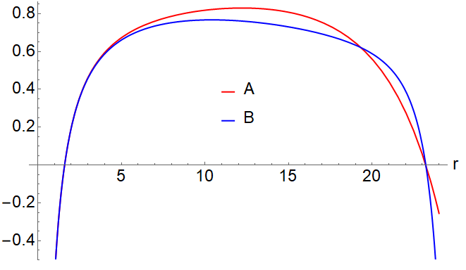
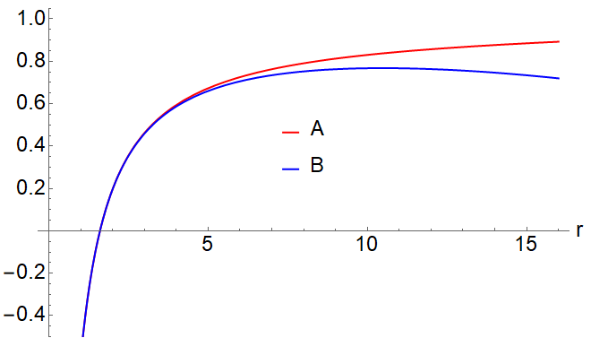
We note that for $\Lambda=0$ the solution exactly corresponds to the stealth Schwarzschild solution with $X=-q^{2}$ and is consistent with the conditions for “Case 1” in Ref. Motohashi and Minamitsuji 2019, and for $r\ll\sqrt{|\zeta/\Lambda|}$ , the solution can be well approximated by the Schwarzschild solution. Thus, on distance scales much shorter than $\sqrt{|\zeta/\Lambda|}$ the gravitational force law can be approximated by the Newtonian one. By choosing $M$ appropriately, no singularity appears between the two event and cosmological horizons. In Fig. 1, the metric functions $A$ and $B$ of the solution Eqs. (69) and (70) are shown by the red and blue curves, respectively. Here, the left and right panels correspond to $\Lambda=10^{-3}$ and $\Lambda=-10^{-3}$ , respectively. The other parameters are chosen to be $\zeta=1$ , $\gamma=2.0$ , $M=0.8$ , and $q=1.0$ . For $\Lambda<0$ , for an appropriate choice of the parameters, $A$ and $B$ cross zero once at the same position, and hence the metric solution Eqs. (69)-(70) represents a BH spacetime. At an intermediate radius, $B$ monotonically increases, while $A$ starts to decrease but never crosses zero again. For $\Lambda>0$ , for an appropriate choice of parameters, $A$ and $B$ cross zero twice at the same positions, which may be identified as the event and cosmological horizons, respectively.

Refer to caption — Figure 1: The metric functions $A$ and $B$ of the solution (68) are shown by the red and blue curves respectively. The left and right panels correspond to $\Lambda=10^{-3}$ and $\Lambda=-10^{-3}$ , respectively. The other parameters are chosen as $\zeta=1$ , $\gamma=2.0$ , $M=0.8$ , and $q=1.0$ .

V.2.2 Model B- $q$

Second, we consider Model B- $q$ given by Eq. (67). The difference from Model A- $q$ (66) is that $F_{0}$ is replaced by $-\beta X$ . In this case, we cannot find an analytic solution and instead need to solve numerically. Following the same procedure, we obtain the set of equations to be integrated numerically

$\displaystyle X^{\prime}$	$\displaystyle=$	$\displaystyle-\frac{8X}{r\gamma}\left[-4q^{2}\gamma\zeta+r^{2}\beta(-4+3\gamma)X^{2}(A+rA^{\prime})+2\gamma X\left(-2\zeta A+r(q^{2}r\beta-2\zeta A^{\prime})\right)\right]$
	$\displaystyle\times$	$\displaystyle\left[-20q^{2}\gamma\zeta+2\left(q^{2}r^{2}\beta(-8+7\gamma)-6r\zeta A\right)X+3r^{2}\beta(-4+3\gamma)AX^{2}\right]^{-1},$
$\displaystyle A^{\prime}$	$\displaystyle=$	$\displaystyle-\frac{2}{rX}\left[8q^{2}\zeta^{2}\gamma^{2}+4\gamma\zeta\left(q^{2}r^{2}\beta(4-5\gamma)+2\gamma\zeta A\right)X+2r^{2}\beta\gamma\left(q^{2}r^{2}\beta(-8+5\gamma)+3(4-3\gamma)\zeta A\right)X^{2}+r^{4}\beta^{2}(4-3\gamma)^{2}AX^{3}\right]$	(72)
	$\displaystyle\times$	$\displaystyle\left[16\gamma^{2}\zeta^{2}-24r^{2}\beta(-2+\gamma)\gamma\zeta X+r^{4}\beta^{2}(32-36\gamma+9\gamma^{2})X^{2}\right]^{-1}.$	(72)

We exclude $\gamma=0$ , which provides the Schwarzschild solution with $q=0$ .

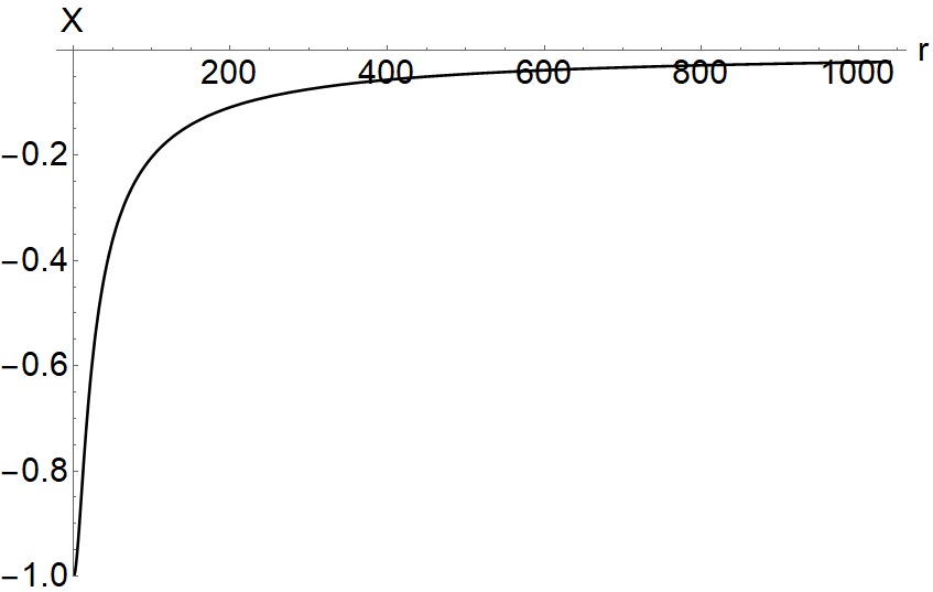
In Fig. 2, for Model B-q (67) the kinetic term $X$ (the left panel) and the metric functions $A$ and $B$ (the right panel) are shown as the functions of $r$ . In the right panel $A$ and $B$ are shown by the red and blue curves respectively. We set the position of the event horizon at $r=1.0$ and $\zeta=1.0$ , $q=1.0$ , $\beta=-10^{-4}$ , and $\gamma=0.05$ , and $X(r=1.0)=-1.0$ as the boundary condition. Throughout the domain of $r$ , $X<0$ and hence the character of $\partial_{\mu}\phi$ is timelike. We also find that $A$ and $B$ cross zero twice at $r=1.0$ and $r\approx 942.0$ , where the latter is interpreted as the cosmological horizon. We note that in contrast to Model A-q (66) with $\Lambda>0$ , no singularity appears outside the cosmological horizon.

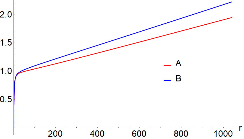
In Fig. 3, for Model B-q (67) the same plots are shown for $\zeta=1.0$ , $q=1.0$ , $\beta=10^{-4}$ , and $\gamma=-0.05$ , and $X(r=1.0)=-1.0$ as the boundary condition. Throughout the domain of $r$ , $X<0$ and hence the character of $\partial_{\mu}\phi$ is timelike. We also find that $A$ and $B$ cross zero only once at $r=1.0$ and monotonically increase. As $\beta$ approaches zero, $A$ and $B$ approach that of the Schwarzschild solution.

V.3 Stability against odd-parity perturbations

If the background scalar field is a function of the radial coordinate, $\phi=qt+\psi(r)$ , the absence of ghost and Laplacian instabilities for the modes with the multipole indices $\ell\geq 2$ requires the conditions

\displaystyle F_{2}>0,\qquad F_{2}-XA_{1}>0,\qquad A_{1}\leq 0.

(73)

Using the ${\cal S}$ -deformation method, the mode stability against the odd-parity perturbations with $\ell\geq 2$ is ensured the function

\displaystyle{\cal S}=\frac{d}{dr_{\ast}}\left[\ln\left(r\sqrt{\frac{A{\cal F}{\cal G}+B{\cal J}^{2}}{A{\cal G}}}\right)\right],

(74)

where the functions ${\cal F}$ , ${\cal G}$ , ${\cal H}$ , and ${\cal J}$ are defined in Eq. (36) of Ref. Takahashi et al. 2019, is finite at both the boundaries, namely both the event horizon and the spatial infinity (or the cosmological horizon, if exists).

In Model A-q (66) with Eq. (56), ${\cal F}={\cal G}={\cal H}=2F_{2}=2\zeta>0$ and ${\cal J}=0$ , and hence the conditions Eq. (73) are automatically satisfied. On the other hand, ${\cal S}=\sqrt{AB}/r$ , which always vanishes at the event horizon. At spatial infinity, ${\cal S}$ always decay for $\gamma>4/3$ and the mode stability can be ensured for this case. For $\gamma<4/3$ the above definition of ${\cal S}$ blows up at the infinity. However, since there might be another choice of ${\cal S}$ which satisfy the desired properties, this does not necessarily mean the instability.

Before closing this section, let us also comment on the strong coupling problem. In Ref. de Rham and Zhang 2019, it was shown that the Schwarzschild -de Sitter BH solutions with a constant kinetic term $X=X_{0}$ suffer the strong coupling problem. In Ref. Motohashi and Mukohyama 2020, it was argued that in the context of the effective field theory the strong coupling problem would be avoided by detuning of the degeneracy conditions (II) for the Case 1 solutions with $X=-q^{2}$ at least in the cosmological asymptotic region, where the apparent Ostrogradski ghost would appear above the cutoff scale of the effective field theory. It has not been explicitly investigated whether the strong coupling problem exist for the BH solutions with a nonconstant kinetic term. In Models A-q and B-q, the Case-1 Schwarzschild solution with $X=-q^{2}$ is recovered in the limits of $\Lambda\to 0$ and $\beta\to 0$ , respectively, but for $\Lambda\neq 0$ and $\beta\neq 0$ the deviation from the constant $X=-q^{2}$ solution becomes more significant in the large distance regions, as $X$ goes to $0$ in the limit of $r\to\infty$ . An explicit analysis about the even-parity perturbations will be necessary to clarify this issue. If there is still the strong coupling problem, it is also interesting to see whether the cure argued in Ref. Motohashi and Mukohyama 2020 could work or not.

VI Conclusions

We investigated static and spherically symmetric BH solutions with a nonconstant kinetic term of the scalar field in shift-symmetric Class Ia quadratic DHOST theories. We used the method developed in Refs. Kobayashi and Hiramatsu 2018; Takahashi et al. 2019. Because of the properties of the DHOST theories, the highest-order derivative terms of the EL equations in static and spherically symmetric backgrounds are degenerate, and combining them gives rise to a constraint relation. Using this constraint relation, the higher-order differential equations can be rewritten in terms of the second-order differential equations.

In order to find analytic BH solutions with a nonconstant $X$ , we had to choose the particular form of the coupling functions. We found Models A, B, and C given by Eqs. (31), (33), and (35), which could provide the analytic BH solutions whose metrics are given by Eqs. (38), (42), and (45), respectively. These solutions have metrics which are neither Schwarzschild nor Schwarzschild - (anti-) de Sitter solutions, but possess only one BH event horizon.

We have also investigated the stability of these BH solutions against the odd-parity perturbations. Our analysis employed the conditions for the absence of the ghost and Laplacian instabilities, and those for the mode stability, which were obtained in Ref. Takahashi et al. 2019. We have shown both that the BH solutions in Models A and C are free from ghost and Laplacian instabilities, and also mode stable, since the function ${\cal S}$ given by Eq. (51) was regular at both the event horizon and the spatial infinity (or the cosmological horizon, if it exists). However, BH solutions in Model B suffer from ghost or Laplacian instabilities.

In § V, we investigated BH solutions with a nonconstant kinetic term for a more general ansatz of the scalar field $\phi=qt+\psi(r)$ with a constant $q$ . We have clarified why it is more difficult to find exact BH solutions compared to $q=0$ . We considered Models A-q (66) and B-q (67) with $A_{1}=A_{2}=0$ . In these examples, adding nontrivial functions of $F_{0}(X)$ modified the asymptotic structure of the spacetime, while the near horizon geometry is close to that of the Schwarzschild BH.

Several issues are left for future work. First, the stability of the BH solutions obtained in this paper against the even-parity perturbations and the possibilities of the strong coupling problems de Rham and Zhang 2019 could be investigated. For coupling functions other than those studied in this paper, one may still be able to construct new BH solutions with a nonconstant kinetic term. Finally, construction of rotating BH solutions with a nonconstant kinetic term will also be important topics for the future.

Acknowledgements.

M.M. was supported by the research grant under the Decree-Law 57/2016 of August 29 (Portugal) through the Fundação para a Ciência e a Tecnologia. J.E. is grateful for the support recieved from CENTRA.

Appendix A BH solutions with a constant $X$

We briefly review the case of the constant kinetic term $X=X_{0}$ .

A.1 The case of $\phi=\phi(r)$

For $\phi=\phi(r)$ , the equations for $B$ and $\Delta E$ reduce to

\displaystyle B^{-1}=\frac{2(F_{2}-X_{0}A_{1})(A+rA^{\prime})}{A(r^{2}F_{0}+2F_{2})},

(75)

and

	$\displaystyle\Delta E$	$\displaystyle=$	$\displaystyle\frac{32(X_{0}A_{1}-F_{2})(A+rA^{\prime})^{2}}{r^{2}(r^{2}F_{0}+2F_{2})(-2A+rA^{\prime})^{2}(-2A_{1}+X_{0}A_{3}+4F_{2X})^{2}}\left[X_{0}A_{3}(3r^{2}F_{0}+4F_{2})+4r^{2}X_{0}F_{0}A_{1X}+8X_{0}F_{2}A_{1X}\right.$		(76)
			$\displaystyle\left.-4r^{2}F_{2}F_{0X}+8r^{2}F_{0}F_{2X}+A_{1}(-2r^{2}F_{0}+4r^{2}X_{0}F_{0X}+8X_{0}F_{2X})\right],$		(76)

where $F_{0,2}(X)$ , $A_{0,1,2,3}(X)$ , and their derivatives are evaluated at $X=X_{0}$ . $\Delta E=0$ , together with the existence of the solution for $B$ , requires

	$\displaystyle X_{0}A_{3}(3r^{2}F_{0}+4F_{2})+4r^{2}X_{0}F_{0}A_{1X}+8X_{0}F_{2}A_{1X}$
	$\displaystyle-4r^{2}F_{2}F_{0X}+8r^{2}F_{0}F_{2X}+A_{1}(-2r^{2}F_{0}+4r^{2}X_{0}F_{0X}+8X_{0}F_{2X})=0.$		(77)

Eq. (A.1) is satisfied for all $r$ , if the coefficients of the $r^{2}$ and $r^{0}$ terms separately vanish, namely,

	$\displaystyle A_{3}$	$\displaystyle=$	$\displaystyle\frac{8F_{0}F_{2}A_{1X}+2A_{1}^{2}(F_{0}-2X_{0}F_{0X})+A_{1}(-4X_{0}F_{0}A_{1X}+4F_{2}F_{0X})}{F_{0}(3X_{0}A_{1}-4F_{2})},$
	$\displaystyle F_{2X}$	$\displaystyle=$	$\displaystyle\frac{F_{2}\left[X_{0}F_{0}A_{1X}+2F_{2}F_{0X}+A_{1}(F_{0}-2X_{0}F_{0X})\right]}{F_{0}(-3X_{0}A_{1}+4F_{2})}.$		(78)

Substituting Eq. (A.1) into $J^{r}=0$ and $E_{A}=0$ provides the degenerate equation $r\left(r^{2}F_{0}+2F_{2}\right)A^{\prime\prime}+4F_{2}A^{\prime}-2rF_{0}A=0$ , which can be solved as

\displaystyle A(r)=C_{1}\left[2F_{2}+\frac{F_{0}}{3}r^{2}-\frac{4M(F_{2}-X_{0}A_{1})}{r}\right],

(79)

where $C_{1}$ and $M$ are integration constants, corresponding to the degrees of freedom for the rescaling of time and the mass of the BH. Substituting into Eq. (75)

\displaystyle B(r)=-\frac{\Lambda}{3}r^{2}+\kappa-\frac{2M}{r},

(80)

where we have defined $\Lambda:=-F_{0}/[2(F_{2}-X_{0}A_{1})]$ , and $\kappa:=F_{2}/(F_{2}-X_{0}A_{1})$ . By choosing $C_{1}$ appropriately, it is possible to make $A=B$ . This solution described the Schwarzschild-(anti-) de Sitter-type solution with the effective cosmological constant $\Lambda$ Motohashi and Minamitsuji 2019; Takahashi et al. 2019. The deficit solid angle is absent ( $\kappa=1$ ) in the case of $A_{1}=0$ , namely in the case that the difference between $c_{gw}$ , the speed of GWs and $c$ , the speed of light is absent, i.e. $c_{gw}=c$ .

A.2 The case of $\phi=qt+\psi(r)$

For $\phi=qt+\psi(r)$ , the equation for $B$ becomes

\displaystyle B^{-1}=\frac{2F_{2}(A+rA^{\prime})}{A(r^{2}F_{0}+2F_{2})},

(81)

and (64) becomes

\displaystyle\Delta_{q}E\propto A_{3}\left[4F_{2}(q^{2}+X_{0}A+rX_{0}A^{\prime})+r^{2}F_{0}(2q^{2}+3X_{0}A+3rX_{0}A^{\prime})\right]-4r^{2}(A+rA^{\prime})(F_{2}F_{0X}-2F_{0}F_{2X}).

(82)

$\Delta E_{q}=0$ sets

	$\displaystyle A^{\prime}(r)$	$\displaystyle=$	$\displaystyle\left[-A_{3}\left(r^{2}(2q^{2}+3X_{0}A)F_{0}+4(q^{2}+X_{0}A)F_{2}\right)+4r^{2}A(F_{2}F_{0X}-2F_{0}F_{2X})\right]$		(83)
		$\displaystyle\times$	$\displaystyle\left[rX_{0}A_{3}(3r^{2}F_{0}+4F_{2})-4r^{3}(F_{2}F_{0X}-2F_{0}F_{2X})\right]^{-1}.$		(83)

Then, $J^{r}=0$ and $E_{A}=0$ yield the degenerate condition

\displaystyle F_{2X}=-\frac{3}{8}X_{0}A_{3}+\frac{F_{2}F_{0X}}{2F_{0}}.

(84)

Substituting Eq. (84) into Eq. (83),

\displaystyle A(r)=-\frac{X_{0}}{q^{2}}\left(\frac{F_{0}}{6F_{2}}r^{2}+1-\frac{2M}{r}\right).

(85)

From Eq. (81), we find

\displaystyle B(r)=\frac{F_{0}}{6F_{2}}r^{2}+1-\frac{2M}{r}.

(86)

If we choose $X_{0}=-q^{2}$ , the solution can be rewritten into the form of the standard Schwarzschild -(anti-) de Sitter solution: $A(r)=B(r)=[F_{0}/(6F_{2})]r^{2}+1-2M/r$ , which corresponds to “Case 1- $\Lambda$ ” in Ref. Motohashi and Minamitsuji 2019.

Appendix B BH solutions with a nonconstant $X$ for $\phi=\phi(r)$

In this appendix, we show the derivation process of BH solutions presented in § IV.

B.1 Model A

We first consider Model A (31). From Eqs. (27) and (23),

\displaystyle X=\left(\frac{4(\gamma_{1}-2\beta_{1})\zeta}{r^{2}\eta_{1}(4n(1-\beta_{1})-3(\gamma_{1}-2\beta_{1}))}\right)^{1/n}.

(87)

Hereafter, for $n>0$ , we impose the conditions Eq. (37), and assume that $\beta_{1}<0$ . Substituting it into Eq. (23),

\displaystyle B=\frac{16n^{2}(1-\beta_{1})A}{\left(4n(1-\beta_{1})-3(\gamma_{1}-2\beta_{1})\right)\left[(4n(1-\beta_{1})-3(\gamma_{1}-2\beta_{1}))A+4nr(1-\beta_{1})A^{\prime}\right]}.

(88)

Then, the degenerate equations $J^{r}=0$ and $E_{A}=0$ yield the second-order differential equation for $A$ , whose solution is given by

\displaystyle A=C_{1}r^{-\left(4n(1-\beta_{1})+6\beta_{1}-3\gamma_{1}\right)/[4n(1-\beta_{1})]}+C_{2}r^{-3(2\beta_{1}-\gamma_{1})/[2n(1-\beta_{1})]},

(89)

with $C_{1}$ and $C_{2}$ being integration constants. Substituting into Eq. (88),

\displaystyle B=\frac{16n^{2}(1-\beta_{1})}{\left(4n(1-\beta_{1})-6\beta_{1}+3\gamma_{1}\right)\left(4n(1-\beta_{1})+6\beta_{1}-3\gamma_{1}\right)}\left(1+\frac{C_{1}}{C_{2}}r^{-\left(4n(1-\beta_{1})-6\beta_{1}+3\gamma_{1}\right)/[4n(1-\beta_{1})]}\right).

(90)

When the conditions Eq. (37) are satisfied, the second term in Eq. (90) becomes negligible in the large distance limit $r\to\infty$ and hence the spatial metric approaches

\displaystyle\frac{\left(4n(1-\beta_{1})-6\beta_{1}+3\gamma_{1}\right)\left(4n(1-\beta_{1})+6\beta_{1}-3\gamma_{1}\right)}{16n^{2}(1-\beta_{1})}dr^{2}+r^{2}(d\theta^{2}+\sin^{2}\theta d\varphi^{2}).

(91)

If the coefficient of the $dr^{2}$ term becomes unity, the 3-space metric reduces to that of an Euclid space $dr^{2}+r^{2}(d\theta^{2}+\sin^{2}\theta d\varphi^{2})$ , and otherwise the solution possesses a deficit solid angle.

In order to avoid the appearance of the deficit solid angle, we also impose

\displaystyle\frac{16n^{2}(1-\beta_{1})}{\left(4n(1-\beta_{1})-6\beta_{1}+3\gamma_{1}\right)\left(4n(1-\beta_{1})+6\beta_{1}-3\gamma_{1}\right)}=1,

(92)

which yields the two roots

\displaystyle\gamma_{1}=\gamma_{1,\pm}=2\beta_{1}\pm\frac{4n}{3}\sqrt{\beta_{1}(\beta_{1}-1)}.

(93)

Since $\gamma_{1,\pm}-2\beta_{1}=\pm 4n\sqrt{\beta_{1}(\beta_{1}-1)}/3$ , only the plus branch is consistent with Eq. (37). For $\gamma_{1}=\gamma_{1,+}$ , choosing $C_{1}=-2M$ and $C_{2}=1$ with $M$ being a constant,

\displaystyle A(r)=r^{2\sqrt{\frac{\beta_{1}}{\beta_{1}-1}}}B(r),\qquad B(r)=1-2Mr^{-1-\sqrt{\frac{\beta_{1}}{\beta_{1}-1}}}.

(94)

The solution of $X$ is given by

\displaystyle X=\left(\frac{4\zeta[-\beta_{1}+\sqrt{\beta_{1}(\beta_{1}-1)}]}{3r^{2}\eta_{1}}\right)^{\frac{1}{n}}.

(95)

The Schwarzschild solution can be obtained in the limit of $\beta_{1}\to 0$ . This is consistent with the fact that as $\beta_{1}\to 0$ and then $\gamma_{1,+}\to 0$ Model A reduces to the scalar-tensor theory with the kinetic term $X^{n}$ .

B.2 Model B

We consider Model B (33). From Eqs. (27) and (23),

\displaystyle X=\left(\frac{-r^{2}(3\gamma_{2}-8n\beta_{2})\Lambda+4\gamma_{2}\zeta}{4\beta_{2}\gamma_{2}}\right)^{1/n}.

(96)

From $n>0$ , we impose the conditions

\displaystyle\beta_{2}>0,\qquad\gamma_{2}>0.

(97)

We also impose $-r^{2}(3\gamma_{2}-8n\beta_{2})\Lambda+4\gamma_{2}\zeta>0$ for any $r$ and hence Eq. (41). Then, the degenerate equations $J^{r}=0$ and $E_{A}=0$ yield the second-order differential equation for $A$ , whose solution is given by

\displaystyle A=r^{-4+\frac{3\gamma_{2}}{4n\beta_{2}}}\left[C_{1}+C_{2}r^{2+\frac{3\gamma_{2}}{4n\beta_{2}}}\right],

(98)

where $C_{1}$ and $C_{2}$ are integration constants. Substituting into the equation for $B$ , we find

\displaystyle B

\displaystyle=

\displaystyle\frac{16n^{2}\beta_{2}^{2}}{64n^{2}\beta_{2}^{2}-9\gamma_{2}^{2}}\left[1+\frac{C_{1}}{C_{2}}r^{-2-\frac{3\gamma_{2}}{4n\beta_{2}}}\right].

(99)

For the absence of the deficit solid angle, we impose $16n^{2}\beta_{2}^{2}/(64n^{2}\beta_{2}^{2}-9\gamma_{2}^{2})=1$ , which with Eq. (97) can be solved as $\gamma_{2}=\frac{4n\beta_{2}}{\sqrt{3}}$ . For this choice of $\beta_{4}$ , by setting $C_{1}=-2M$ and $C_{2}=1$ , we find

\displaystyle A(r)=r^{-2+2\sqrt{3}}B(r),\qquad B(r)=1-\frac{2M}{r^{2+\sqrt{3}}}.

(100)

In the metric solution Eq. (42), the event horizon exists at $A=B=0$ . The solution to $X$ is given by

\displaystyle X=\left(\frac{4\zeta-(3-2\sqrt{3})r^{2}\Lambda}{4\beta_{2}}\right)^{\frac{1}{n}}.

(101)

B.3 Model C

We then consider Model C (35). From Eqs. (27) and (23),

\displaystyle X=\left(-\frac{(2n-3)\beta_{3}+4n\gamma_{3}}{4(1-2n)\beta_{3}\gamma_{3}}\Lambda r^{2}\right)^{1/n}.

(102)

For $n>0$ , we impose the conditions (44). The solution for $B$ is given by

\displaystyle B=\frac{4n^{2}(\beta_{3}-\gamma_{3})\gamma_{3}A}{\left[(2n-3)\beta_{3}+4n\gamma_{3}\right]\left[\left((2n+3)\beta_{3}-8n\gamma_{3}\right)A+2nr(\beta_{3}-\gamma_{3})A^{\prime}\right]}.

(103)

The degenerate equations $J^{r}=0$ and $E_{A}=0$ yield the second-order differential equation for $A$ , whose solution is given by

\displaystyle A=C_{1}r^{\frac{(-3+4n)\beta_{3}+2n\gamma_{3}}{n(\beta_{3}-\gamma_{3})}}+C_{2}r^{-\frac{3\beta_{3}+2n\beta_{3}-8n\gamma_{3}}{2n(\beta_{3}-\gamma_{3})}},

(104)

where $C_{1}$ and $C_{2}$ are integration constants. Substituting into the equation for $B$ , we find

\displaystyle B

\displaystyle=

\displaystyle\frac{4n^{2}\gamma_{3}(\beta_{3}-\gamma_{3})}{\left((10n-3)\beta_{3}-4n\gamma_{3}\right)\left((-3+2n)\beta_{3}+4n\gamma_{3}\right)}\left[1+\frac{C_{2}}{C_{1}}r^{\frac{3\beta_{3}-10n\beta_{3}+4n\gamma_{3}}{2n(\beta_{3}-\gamma_{3})}}\right].

(105)

For the absence of the deficit solid angle, we impose $4n^{2}\gamma_{3}(\beta_{3}-\gamma_{3})/[\left((10n-3)\beta_{3}-4n\gamma_{3}\right)\left((-3+2n)\beta_{3}+4n\gamma_{3}\right)]=1$ , which with Eq. (97) can be solved as

\displaystyle\gamma_{3}=\frac{\beta_{3}}{6n}\left(7n\pm\sqrt{27+n(-108+109n)}\right).

(106)

We note that $27+n(-108+109n)>0$ for $0<n<1/2$ , and only the plus branch satisfies Eq. (44) and hence the minus branch is excluded in the rest of this subsection. For this choice of $\gamma_{3}$ , by setting $C_{2}=-2M$ and $C_{1}=1$ , we find

\displaystyle A(r)=r^{2\frac{-3+5n+\sqrt{27+n(-108+109n)}}{3(1-2n)}}B(r),\qquad B(r)=1-2Mr^{-\frac{6-13n+\sqrt{27+n(-108+109n)}}{3(1-2n)}}.

(107)

In the metric solution Eq. (45), the event horizon exists at $A=B=0$ . For $n=3/7$ , Eq. (45) reduces to

\displaystyle A(r)=B(r),\qquad B(r)=1-\frac{2M}{r^{3}},

(108)

which describes the asymptotically flat BH solutions. The solution to $X$ is given by

\displaystyle X=\left(-\frac{n(-6+13n+\sqrt{27+n(-108+109n)})}{2(1-2n)(-3+10n)\beta_{3}}\Lambda r^{2}\right)^{1/n},

(109)

where the combination inside the round bracket is positive for $0<n<1/2$ , $\beta_{3}>0$ , and $\Lambda<0$ . The solution has no Schwarzschild limit, as Model C has no limit to GR and to the classic scalar-tensor theories.

B.4 Model D

Although we do not consider them in details in the text, we will introduce two other models here for reference.

For Model D (48), by substituting into Eqs. (27) and (23), we obtain

	$\displaystyle\Delta E$	$\displaystyle=$	$\displaystyle\frac{(-4\zeta+r^{2}\eta_{4}X)(8X+rX^{\prime})\left(8rXA^{\prime}+A(8X+3rX^{\prime})\right)^{2}}{16r^{2}X^{2}(2\zeta+2\beta_{4}\sqrt{X}+r^{2}\eta_{4}X)(rA^{\prime}-2A)^{2}}=0,$		(110)
	$\displaystyle B$	$\displaystyle=$	$\displaystyle\frac{32AX^{2}(2\zeta+2\beta_{4}\sqrt{X}+r^{2}\eta_{4}X)}{\zeta(8X+rX^{\prime})\left(8rXA^{\prime}+A(8X+3rX^{\prime})\right)}.$		(111)

In order for Eq. (110) to be satisfied while allowing a solution of $B$ to exist, we impose

\displaystyle X=\frac{4\zeta}{r^{2}\eta_{1}}.

(112)

Substituting this into Eq. (111), we obtain

\displaystyle B=\frac{16A}{3\zeta(A+4rA^{\prime})}\left(3\zeta+\frac{2\beta_{4}}{r}\sqrt{\frac{\zeta}{\eta_{4}}}\right).

(113)

Then, the degenerate equations $J^{r}=0$ and $E_{A}=0$ yield the second-order differential equation for $A$

\displaystyle 2r\left[4r\left(3r\zeta+2\beta_{4}\sqrt{\frac{\zeta}{\eta_{4}}}\right)A^{\prime\prime}+\left(-3r\zeta+6\beta_{4}\sqrt{\frac{\zeta}{\eta_{4}}}\right)A^{\prime}\right]-\left(9r\zeta+2\beta_{4}\sqrt{\frac{\zeta}{\eta_{4}}}\right)A=0,

(114)

Finding the solution of $A$ and substituting it back into Eq. (113), we obtain

\displaystyle B=\frac{A}{r^{3/2}}=\frac{16}{7}+\frac{32\beta_{4}}{9\zeta r}\sqrt{\frac{\zeta}{\eta_{4}}}-\frac{2M}{r^{7/4}}.

(115)

The solution is neither Schwarzschild nor Schwarzschild (anti-) de Sitter. Since $A$ and $B$ cross zero once and at the same place, the solution describes a BH spacetime. As $r\to\infty$ , $B\to 16/7$ and hence the three-dimensional space has a deficit solid angle.

B.5 Model E

Another example we consider is Model E (49). From Eqs. (27) and (23),

\displaystyle X=\frac{2}{r}\left(\frac{(r^{2}\alpha_{5}-\gamma_{5})\zeta}{5\alpha_{5}\gamma_{5}}\right)^{1/2}.

(116)

For $n>0$ , we impose the conditions

\displaystyle\zeta>0,\qquad\alpha_{5}>0,\qquad\gamma_{5}>0,

(117)

and the point where $r^{2}\alpha_{5}-\gamma_{5}=0$ is located inside the event horizon (see below). Substituting it into Eq. (23),

\displaystyle B=\frac{r^{2}\alpha_{5}(2r^{2}\alpha_{5}+3\gamma_{5})(r^{2}\alpha_{5}+4\gamma_{5})A}{\gamma_{5}(r^{2}\alpha_{5}+3\gamma_{5})\left[(r^{2}\alpha_{5}+\gamma_{5})A+r(r^{2}\alpha_{5}+4\gamma_{5})A^{\prime}\right]}.

(118)

The degenerate equations $J^{r}=0$ and $E_{A}=0$ yield the second-order differential equation for $A$ , whose solution is given by

	$\displaystyle A$	$\displaystyle=$	$\displaystyle\frac{C_{2}}{21\sqrt{r}(r^{2}\alpha_{5}+4\gamma_{5})^{3/4}}\left[7\left(2r^{4}\alpha_{5}^{2}-19r^{2}\alpha_{5}\gamma_{5}-108\gamma_{5}^{2}+3C_{1}r^{1/4}(r^{2}\alpha_{5}+4\gamma_{5})^{3/8}\right)\right.$		(119)
			$\displaystyle\left.+80\times 2^{1/4}\alpha_{5}\gamma_{5}r^{2}\left(4+\frac{\alpha_{5}r^{2}}{\gamma_{5}}\right)^{3/8}{}_{2}F_{1}\left[\frac{3}{8},\frac{7}{8},\frac{15}{8};-\frac{\alpha_{5}}{4\gamma_{5}}r^{2}\right]\right].$		(119)

with $C_{1}$ and $C_{2}$ being integration constants, and ${}_{2}F_{1}$ represents the hypergeometric function. Substituting into Eq. (118),

	$\displaystyle B$	$\displaystyle=$	$\displaystyle\frac{r^{2}\alpha_{5}}{21\gamma_{5}(r^{2}\alpha_{5}+3\gamma_{5})^{2}}\left[7\left(2r^{4}\alpha_{5}^{2}-19r^{2}\alpha_{5}\gamma_{5}-108\gamma_{5}^{2}+3C_{1}r^{1/4}(r^{2}\alpha_{5}+4\gamma_{5})^{3/8}\right)\right.$		(120)
			$\displaystyle\left.+80\times 2^{1/4}\alpha_{5}\gamma_{5}r^{2}\left(4+\frac{\alpha_{5}r^{2}}{\gamma_{5}}\right)^{3/8}{}_{2}F_{1}\left[\frac{3}{8},\frac{7}{8},\frac{15}{8};-\frac{\alpha_{5}}{4\gamma_{5}}r^{2}\right]\right].$		(120)

By choosing $C_{2}=\frac{\alpha_{5}}{\gamma_{5}}$ ,

\displaystyle A=\frac{\left(\alpha_{5}r^{2}+3\gamma_{5}\right)^{2}}{r^{5/2}\left(\alpha_{5}r^{2}+4\gamma_{5}\right)^{3/4}}B.

(121)

$A$ and $B$ cross zero once at the same place and monotonically increase, and hence the solution describes a BH spacetime with an event horizon.

Appendix C BH solutions with a nonconstant $X$ for $\phi=qt+\psi(r)$

In this appendix, we show the derivation process of BH solutions in Models A-q (66) and B-q (67).

C.1 Model A-q

Eqs. (61) and (64) can then be rewritten as

$\displaystyle\frac{1}{B}$	$\displaystyle=$	$\displaystyle\frac{\zeta\left(8X+\gamma rX^{\prime}\right)\left[8X^{2}(A+rA^{\prime})+r\gamma\left(4q^{2}+3AX\right)X^{\prime}\right]}{32(2\zeta-r^{2}\Lambda)AX^{3}},$
$\displaystyle\Delta_{q}E$	$\displaystyle=$	$\displaystyle-A^{2}(8X+r\gamma X^{\prime})^{2}\left(8X^{2}(A+rA^{\prime})+r\gamma(4q^{2}+3AX)X^{\prime}\right)$	(122)
	$\displaystyle\times$	$\displaystyle\left[8X\left(2q^{2}(2\zeta-r^{2}\Lambda)+(4\zeta-3r^{2}\Lambda)X(A+rA^{\prime})\right)+\gamma r\left(2q^{2}(10\zeta-7r^{2}\Lambda)+3(4\zeta-3r^{2}\Lambda)AX\right)X^{\prime}\right]$
	$\displaystyle\times$	$\displaystyle\left[16\gamma r^{2}(2\zeta-r^{2}\Lambda)X(4q^{2}+2AX-rXA^{\prime})^{2}\left(4q^{4}\gamma+X\left(2q^{2}\gamma A-q^{2}r\gamma A^{\prime}+A^{2}(8X+r\gamma X^{\prime})\right)\right)\right]^{-1}.$

The equation $\Delta_{q}E=0$ gives

\displaystyle X^{\prime}

\displaystyle=

\displaystyle-\frac{8X\left[2q^{2}(2\zeta-r^{2}\Lambda)+(4\zeta-3r^{2}\Lambda)(AX+rXA^{\prime})\right]}{r\gamma\left(2q^{2}(10\zeta-7r^{2}\Lambda)+3(4\zeta-3r^{2}\Lambda)AX\right)},

(123)

and therefore eliminating $X^{\prime}$

\displaystyle B=-\frac{AX\left[2q^{2}(10\zeta-7r^{2}\Lambda)+3(4\zeta-3r^{2}\Lambda)AX\right]^{2}}{4q^{2}\zeta(4\zeta-3r^{2}\Lambda)\left(4q^{2}+2AX-rXA^{\prime}\right)^{2}}.

(124)

The degenerate equations (62) and (63) reduce to an equation for $A$ :

	$\displaystyle A^{\prime}$	$\displaystyle=$	$\displaystyle\left[4q^{2}\left(-4(-4+3\gamma)\zeta^{2}-10r^{2}(2-3\gamma)\Lambda\zeta+3r^{4}(2-5\gamma)\Lambda^{2}\right)-2(4\zeta-3r^{2}\Lambda)\left((-8+6\gamma)\zeta+3r^{2}(2-3\gamma)\Lambda\right)AX\right]$		(125)
		$\displaystyle\times$	$\displaystyle\left[r(-4+3\gamma)(4\zeta-3r^{2}\Lambda)^{2}X\right]^{-1}.$		(125)

We note that our analysis excludes the case of $\gamma=4/3$ . We find the exact BH solutions expressed by the following nonconstant kinetic term and the metric functions

$\displaystyle X$	$\displaystyle=$	$\displaystyle-q^{2}\left(1-\frac{3r^{2}\Lambda}{4\zeta}\right)^{-\frac{4}{4-3\gamma}},$
$\displaystyle A$	$\displaystyle=$	$\displaystyle-\frac{1}{3r(3\gamma-4)}\left(1-\frac{3r^{2}\Lambda}{4\zeta}\right)^{\frac{3\gamma}{8-6\gamma}}\left\{6M(-4+3\gamma)+4r(2-5\gamma)\,\,{}_{2}F_{1}\left[\frac{1}{2},-\frac{8-3\gamma}{8-6\gamma},\frac{3}{2};\frac{3r^{2}\Lambda}{4\zeta}\right]\right.$	(126)
		$\displaystyle\left.+2r(2+5\gamma)\,\,{}_{2}F_{1}\left[\frac{1}{2},-\frac{3\gamma}{8-6\gamma},\frac{3}{2};\frac{3r^{2}\Lambda}{4\zeta}\right]+\gamma r\,\,{}_{2}F_{1}\left[\frac{1}{2},\frac{3}{2}+\frac{2}{-4+3\gamma},\frac{3}{2};\frac{3r^{2}\Lambda}{4\zeta}\right]\right\}.$	(126)

$B$ can be calculated by obtained $A$ and $X$ into Eq. (124), namely

\displaystyle\frac{B}{A}=\frac{(4-3\gamma)^{2}\zeta^{2}}{\left((4-3\gamma)\zeta+3r^{2}(\gamma-1)\Lambda\right)^{2}}\left(1-\frac{3r^{2}\Lambda}{4\zeta}\right)^{3+\frac{4}{3\gamma-4}}.

(127)

C.2 Model B-q

Eqs. (61) and (64) can then be rewritten as

$\displaystyle\frac{1}{B}$	$\displaystyle=$	$\displaystyle-\left[\zeta(8X+r\gamma X^{\prime})\left(4r(2X^{2}A^{\prime}+q^{2}\gamma X^{\prime})+AX(8X+3r\gamma X^{\prime})\right)\right]$
	$\displaystyle\times$	$\displaystyle\left[32AX^{3}(2\zeta-r^{2}\beta X)\right]^{-1},$
$\displaystyle\Delta_{q}E$	$\displaystyle=$	$\displaystyle A^{2}(8X+r\gamma X^{\prime})^{2}\left(4r(2X^{2}A^{\prime}+q^{2}\gamma X^{\prime})+AX(8X+3r\gamma X^{\prime})\right)$	(128)
	$\displaystyle\times$	$\displaystyle\left[\gamma X^{2}\left(16r\left(\beta q^{2}r-2\zeta A^{\prime}\right)+A\left(3\beta(3\gamma-4)r^{3}X^{\prime}-32\zeta\right)\right)+8\beta(3\gamma-4)r^{2}X^{3}\left(rA^{\prime}+A\right)\right.$
		$\displaystyle\left.+2\gamma X\left(X^{\prime}\left(\beta(7\gamma-8)q^{2}r^{3}-6\gamma\zeta rA\right)-16\zeta q^{2}\right)-20\gamma^{2}\zeta q^{2}rX^{\prime}\right]$
	$\displaystyle\times$	$\displaystyle\left[16\gamma^{2}r^{2}X\left(\beta r^{2}X-2\zeta\right)\left(-rXA^{\prime}+2A(r)X+4q^{2}\right)^{2}\right.$
		$\displaystyle\left.\times\left(\gamma q^{2}rXA^{\prime}-2\gamma q^{2}AX-A^{2}X\left(\gamma rX^{\prime}+8X\right)-4\gamma q^{4}\right)\right]^{-1}.$

The equation $\Delta_{q}E=0$ gives

	$\displaystyle X^{\prime}$	$\displaystyle=$	$\displaystyle-\frac{8X}{r\gamma}\left[-4q^{2}\gamma\zeta+r^{2}\beta(-4+3\gamma)X^{2}(A+rA^{\prime})+2\gamma X\left(-2\zeta A+r(q^{2}r\beta-2\zeta A^{\prime})\right)\right]$		(129)
		$\displaystyle\times$	$\displaystyle\left[-20q^{2}\gamma\zeta+2\left(q^{2}r^{2}\beta(-8+7\gamma)-6r\zeta A\right)X+3r^{2}\beta(-4+3\gamma)AX^{2}\right]^{-1},$		(129)

and eliminating $X^{\prime}$

	$\displaystyle B$	$\displaystyle=$	$\displaystyle-\left[AX\left(-2X\left(\beta(7\gamma-8)q^{2}r^{2}-6A\gamma\zeta\right)+3A\beta(4-3\gamma)r^{2}X^{2}+20\gamma\zeta q^{2}\right)^{2}\right]$		(130)
		$\displaystyle\times$	$\displaystyle\left[4\gamma\zeta q^{2}\left(4q^{2}+2AX-rXA^{\prime}\right)^{2}\left(4\gamma\zeta+\beta(4-3\gamma)r^{2}X\right)\right]^{-1}.$		(130)

The degenerate equations (62) and (63) reduce to an equation for $A$ :

	$\displaystyle A^{\prime}$	$\displaystyle=$	$\displaystyle-\frac{2}{rX}\left[8q^{2}\zeta^{2}\gamma^{2}+4\gamma\zeta\left(q^{2}r^{2}\beta(4-5\gamma)+2\gamma\zeta A\right)X+2r^{2}\beta\gamma\left(q^{2}r^{2}\beta(5-8\gamma)+3(4-3\gamma)\zeta A\right)X^{2}+r^{4}\beta^{2}(4-3\gamma)^{2}AX^{3}\right]$		(131)
		$\displaystyle\times$	$\displaystyle\left[16\gamma^{2}\zeta^{2}-24r^{2}\beta(\gamma-2)\gamma\zeta X+r^{4}\beta^{2}(32-36\gamma+9\gamma^{2})X^{2}\right]^{-1}.$		(131)

The combined equations (129) and (131) are solved numerically.

In the vicinity of the BH horizon $r=r_{h}$ , the solution for $A$ , $B$ , and $X$ can be decomposed as

$\displaystyle A$	$\displaystyle=$	$\displaystyle a_{1}(r-r_{h})+{\cal O}\left[(r-r_{h})^{2}\right],$
$\displaystyle B$	$\displaystyle=$	$\displaystyle b_{1}(r-r_{h})+{\cal O}\left[(r-r_{h})^{2}\right],$
$\displaystyle X$	$\displaystyle=$	$\displaystyle x_{0}+x_{1}(r-r_{h})+{\cal O}\left[(r-r_{h})^{2}\right],$	(132)

where

$\displaystyle a_{1}$	$\displaystyle=$	$\displaystyle-\left[4\gamma q^{2}\left(4\gamma\zeta^{2}+\beta^{2}(5\gamma-8)r_{h}^{4}x_{0}^{2}+2\beta(4-5\gamma)\zeta r_{h}^{2}x_{0}\right)\right]$
	$\displaystyle\times$	$\displaystyle\left[r_{h}x_{0}\left(16\gamma^{2}\zeta^{2}+\beta^{2}\left(9\gamma^{2}-36\gamma+32\right)r_{h}^{4}x_{0}^{2}-24\beta(\gamma-2)\gamma\zeta r_{h}^{2}x_{0}\right)\right]^{-1},$
$\displaystyle b_{1}$	$\displaystyle=$	$\displaystyle-\frac{\left(\beta(3\gamma-8)r_{h}^{2}x_{0}-4\gamma\zeta\right)\left(4\gamma\zeta^{2}+\beta^{2}(5\gamma-8)r_{h}^{4}x_{0}^{2}+2\beta(4-5\gamma)\zeta r_{h}^{2}x_{0}\right)}{16r_{h}\zeta(r_{h}^{2}x_{0}\beta(\gamma-2)-\gamma\zeta)^{2}},$
$\displaystyle x_{1}$	$\displaystyle=$	$\displaystyle\frac{8r_{h}x_{0}^{2}\beta}{r_{h}^{2}x_{0}\beta(3\gamma-8)-4\gamma\zeta},$	(133)

which are used for the boundary conditions for the numerical integration. In the limit of $\beta=0$ , $x_{1}=0$ , $a_{1}=-q^{2}/(r_{h}x_{0})$ , and $b_{1}=1/r_{h}$ , which represents the Schwarzschild spacetime with $X=x_{0}$ .

References

Berti et al. (2015) E. Berti et al., Class. Quant. Grav. 32, 243001 (2015), arXiv:1501.07274 [gr-qc] .
Woodard (2015) R. P. Woodard, Scholarpedia 10, 32243 (2015), arXiv:1506.02210 [hep-th] .
Motohashi et al. (2016a) H. Motohashi, K. Noui, T. Suyama, M. Yamaguchi, and D. Langlois, JCAP 1607, 033 (2016a), arXiv:1603.09355 [hep-th] .
Langlois and Noui (2016) D. Langlois and K. Noui, JCAP 1602, 034 (2016), arXiv:1510.06930 [gr-qc] .
Crisostomi et al. (2016) M. Crisostomi, K. Koyama, and G. Tasinato, JCAP 1604, 044 (2016), arXiv:1602.03119 [hep-th] .
Ben Achour et al. (2016a) J. Ben Achour, D. Langlois, and K. Noui, Phys. Rev. D93, 124005 (2016a), arXiv:1602.08398 [gr-qc] .
Ben Achour et al. (2016b) J. Ben Achour, M. Crisostomi, K. Koyama, D. Langlois, K. Noui, and G. Tasinato, JHEP 12, 100 (2016b), arXiv:1608.08135 [hep-th] .
Crisostomi and Koyama (2018) M. Crisostomi and K. Koyama, Phys. Rev. D97, 021301 (2018), arXiv:1711.06661 [astro-ph.CO] .
Langlois et al. (2018) D. Langlois, R. Saito, D. Yamauchi, and K. Noui, Phys. Rev. D97, 061501 (2018), arXiv:1711.07403 [gr-qc] .
Langlois (2019) D. Langlois, Int. J. Mod. Phys. D28, 1942006 (2019), arXiv:1811.06271 [gr-qc] .
Kobayashi (2019) T. Kobayashi, Rept. Prog. Phys. 82, 086901 (2019), arXiv:1901.07183 [gr-qc] .
Langlois et al. (2017) D. Langlois, M. Mancarella, K. Noui, and F. Vernizzi, JCAP 1705, 033 (2017), arXiv:1703.03797 [hep-th] .
Dima and Vernizzi (2018) A. Dima and F. Vernizzi, Phys. Rev. D97, 101302 (2018), arXiv:1712.04731 [gr-qc] .
Creminelli et al. (2018) P. Creminelli, M. Lewandowski, G. Tambalo, and F. Vernizzi, JCAP 1812, 025 (2018), arXiv:1809.03484 [astro-ph.CO] .
Saltas and Lopes (2019) I. D. Saltas and I. Lopes, Phys. Rev. Lett. 123, 091103 (2019), arXiv:1909.02552 [astro-ph.CO] .
Motohashi and Minamitsuji (2018) H. Motohashi and M. Minamitsuji, Phys. Lett. B781, 728 (2018), arXiv:1804.01731 [gr-qc] .
Motohashi and Minamitsuji (2019) H. Motohashi and M. Minamitsuji, Phys. Rev. D99, 064040 (2019), arXiv:1901.04658 [gr-qc] .
Babichev and Charmousis (2014) E. Babichev and C. Charmousis, JHEP 08, 106 (2014), arXiv:1312.3204 [gr-qc] .
Kobayashi and Tanahashi (2014) T. Kobayashi and N. Tanahashi, PTEP 2014, 073E02 (2014), arXiv:1403.4364 [gr-qc] .
Ben Achour and Liu (2019) J. Ben Achour and H. Liu, Phys. Rev. D99, 064042 (2019), arXiv:1811.05369 [gr-qc] .
Takahashi et al. (2019) K. Takahashi, H. Motohashi, and M. Minamitsuji, Phys. Rev. D100, 024041 (2019), arXiv:1904.03554 [gr-qc] .
Minamitsuji and Edholm (2019) M. Minamitsuji and J. Edholm, Phys. Rev. D100, 044053 (2019), arXiv:1907.02072 [gr-qc] .
Babichev et al. (2018) E. Babichev, C. Charmousis, G. Esposito-Farese, and A. Lehebel, Phys. Rev. Lett. 120, 241101 (2018), arXiv:1712.04398 [gr-qc] .
Charmousis et al. (2019a) C. Charmousis, M. Crisostomi, R. Gregory, and N. Stergioulas, Phys. Rev. D100, 084020 (2019a), arXiv:1903.05519 [hep-th] .
Charmousis et al. (2019b) C. Charmousis, M. Crisostomi, D. Langlois, and K. Noui, Class. Quant. Grav. 36, 235008 (2019b), arXiv:1907.02924 [gr-qc] .
de Rham and Zhang (2019) C. de Rham and J. Zhang, Phys. Rev. D100, 124023 (2019), arXiv:1907.00699 [hep-th] .
Kobayashi and Hiramatsu (2018) T. Kobayashi and T. Hiramatsu, Phys. Rev. D97, 104012 (2018), arXiv:1803.10510 [gr-qc] .
Rinaldi (2012) M. Rinaldi, Phys. Rev. D86, 084048 (2012), arXiv:1208.0103 [gr-qc] .
Anabalon et al. (2014) A. Anabalon, A. Cisterna, and J. Oliva, Phys. Rev. D89, 084050 (2014), arXiv:1312.3597 [gr-qc] .
Minamitsuji (2014) M. Minamitsuji, Phys. Rev. D89, 064017 (2014), arXiv:1312.3759 [gr-qc] .
Sotiriou and Zhou (2014a) T. P. Sotiriou and S.-Y. Zhou, Phys. Rev. Lett. 112, 251102 (2014a), arXiv:1312.3622 [gr-qc] .
Sotiriou and Zhou (2014b) T. P. Sotiriou and S.-Y. Zhou, Phys. Rev. D90, 124063 (2014b), arXiv:1408.1698 [gr-qc] .
Babichev et al. (2017) E. Babichev, C. Charmousis, and A. Lehebel, JCAP 1704, 027 (2017), arXiv:1702.01938 [gr-qc] .
Ben Achour et al. (2019) J. Ben Achour, H. Liu, and S. Mukohyama, (2019), arXiv:1910.11017 [gr-qc] .
Klein and Roest (2016) R. Klein and D. Roest, JHEP 07, 130 (2016), arXiv:1604.01719 [hep-th] .
Motohashi et al. (2018a) H. Motohashi, T. Suyama, and M. Yamaguchi, J. Phys. Soc. Jap. 87, 063401 (2018a), arXiv:1711.08125 [hep-th] .
Motohashi et al. (2018b) H. Motohashi, T. Suyama, and M. Yamaguchi, JHEP 06, 133 (2018b), arXiv:1804.07990 [hep-th] .
Horndeski (1974) G. W. Horndeski, Int. J. Theor. Phys. 10, 363 (1974).
Deffayet et al. (2009a) C. Deffayet, G. Esposito-Farese, and A. Vikman, Phys. Rev. D79, 084003 (2009a), arXiv:0901.1314 [hep-th] .
Deffayet et al. (2009b) C. Deffayet, S. Deser, and G. Esposito-Farese, Phys. Rev. D80, 064015 (2009b), arXiv:0906.1967 [gr-qc] .
Deffayet et al. (2011) C. Deffayet, X. Gao, D. A. Steer, and G. Zahariade, Phys. Rev. D84, 064039 (2011), arXiv:1103.3260 [hep-th] .
Kobayashi et al. (2011) T. Kobayashi, M. Yamaguchi, and J. Yokoyama, Prog. Theor. Phys. 126, 511 (2011), arXiv:1105.5723 [hep-th] .
Gleyzes et al. (2015) J. Gleyzes, D. Langlois, F. Piazza, and F. Vernizzi, Phys. Rev. Lett. 114, 211101 (2015), arXiv:1404.6495 [hep-th] .
Abbott et al. (2017a) B. Abbott et al. (Virgo, LIGO Scientific), Phys. Rev. Lett. 119, 161101 (2017a), arXiv:1710.05832 [gr-qc] .
Abbott et al. (2017b) B. P. Abbott et al. (GROND, SALT Group, OzGrav, DFN, INTEGRAL, Virgo, Insight-Hxmt, MAXI Team, Fermi-LAT, J-GEM, RATIR, IceCube, CAASTRO, LWA, ePESSTO, GRAWITA, RIMAS, SKA South Africa/MeerKAT, H.E.S.S., 1M2H Team, IKI-GW Follow-up, Fermi GBM, Pi of Sky, DWF (Deeper Wider Faster Program), Dark Energy Survey, MASTER, AstroSat Cadmium Zinc Telluride Imager Team, Swift, Pierre Auger, ASKAP, VINROUGE, JAGWAR, Chandra Team at McGill University, TTU-NRAO, GROWTH, AGILE Team, MWA, ATCA, AST3, TOROS, Pan-STARRS, NuSTAR, ATLAS Telescopes, BOOTES, CaltechNRAO, LIGO Scientific, High Time Resolution Universe Survey, Nordic Optical Telescope, Las Cumbres Observatory Group, TZAC Consortium, LOFAR, IPN, DLT40, Texas Tech University, HAWC, ANTARES, KU, Dark Energy Camera GW-EM, CALET, Euro VLBI Team, ALMA), Astrophys. J. 848, L12 (2017b), arXiv:1710.05833 [astro-ph.HE] .
Abbott et al. (2017c) B. P. Abbott et al. (Virgo, Fermi-GBM, INTEGRAL, LIGO Scientific), Astrophys. J. 848, L13 (2017c), arXiv:1710.05834 [astro-ph.HE] .
Creminelli and Vernizzi (2017) P. Creminelli and F. Vernizzi, Phys. Rev. Lett. 119, 251302 (2017), arXiv:1710.05877 [astro-ph.CO] .
Ezquiaga and Zumalacarregui (2017) J. M. Ezquiaga and M. Zumalacarregui, Phys. Rev. Lett. 119, 251304 (2017), arXiv:1710.05901 [astro-ph.CO] .
Baker et al. (2017) T. Baker, E. Bellini, P. G. Ferreira, M. Lagos, J. Noller, and I. Sawicki, Phys. Rev. Lett. 119, 251301 (2017), arXiv:1710.06394 [astro-ph.CO] .
Sakstein and Jain (2017) J. Sakstein and B. Jain, Phys. Rev. Lett. 119, 251303 (2017), arXiv:1710.05893 [astro-ph.CO] .
de Rham and Melville (2018) C. de Rham and S. Melville, Phys. Rev. Lett. 121, 221101 (2018), arXiv:1806.09417 [hep-th] .
Kobayashi et al. (2015) T. Kobayashi, Y. Watanabe, and D. Yamauchi, Phys. Rev. D91, 064013 (2015), arXiv:1411.4130 [gr-qc] .
Motohashi et al. (2016b) H. Motohashi, T. Suyama, and K. Takahashi, Phys. Rev. D94, 124021 (2016b), arXiv:1608.00071 [gr-qc] .
Carter (1971) B. Carter, Phys. Rev. Lett. 26, 331 (1971).
Chase (1970) J. E. Chase, Commun. Math. Phys. 19, 276 (1970).
Bekenstein (1972) J. D. Bekenstein, Phys. Rev. Lett. 28, 452 (1972).
Bekenstein (1995) J. D. Bekenstein, Phys. Rev. D51, R6608 (1995).
Graham and Jha (2014a) A. A. H. Graham and R. Jha, Phys. Rev. D89, 084056 (2014a), [Erratum: Phys. Rev.D92,no.6,069901(2015)], arXiv:1401.8203 [gr-qc] .
Graham and Jha (2014b) A. A. H. Graham and R. Jha, Phys. Rev. D90, 041501 (2014b), arXiv:1407.6573 [gr-qc] .
Minamitsuji and Motohashi (2018) M. Minamitsuji and H. Motohashi, Phys. Rev. D98, 084027 (2018), arXiv:1809.06611 [gr-qc] .
Babichev et al. (2015) E. Babichev, C. Charmousis, and M. Hassaine, JCAP 1505, 031 (2015), arXiv:1503.02545 [gr-qc] .
Motohashi and Mukohyama (2020) H. Motohashi and S. Mukohyama, JCAP 2001, 030 (2020), arXiv:1912.00378 [gr-qc] .

Black holes with a nonconstant kinetic term in degenerate higher-order scalar tensor theories

Abstract

I Introduction

II The DHOST Theories

III Static and spherically symmetric solutions in the shift-symmetric DHOST theories

III.1 The shift-symmetric quadratic DHOST theores

III.2 Static and spherically symmetric spacetime

III.3 The degenerate equations

III.4 The cases of a nonconstant XX

Special case 1: A1=0A_{1}=0 and A3=0A_{3}=0

Special case 2: F0=0F_{0}=0 and A3=0A_{3}=0

Models in the Class Ia DHOST theories

IV Exact black hole solutions and stability against the odd-parity perturbations

IV.1 Exact black hole solutions

IV.1.1 Model A

IV.1.2 Model B

IV.1.3 Model C

IV.2 A short summary

IV.3 Stability against odd-parity perturbations

IV.3.1 Model A

IV.3.2 Model B

IV.3.3 Model C

V The case of the linearly time-dependent scalar field

V.1 Solving the equations of motion

V.2 BH solutions with a nonconstant XX

V.2.1 Model A-qq

V.2.2 Model B-qq

V.3 Stability against odd-parity perturbations

VI Conclusions

Acknowledgements.

Appendix A BH solutions with a constant XX

A.1 The case of ϕ=ϕ⁡(r)\phi=\phi(r)

A.2 The case of ϕ=q​t+ψ⁡(r)\phi=qt+\psi(r)

Appendix B BH solutions with a nonconstant XX for ϕ=ϕ⁡(r)\phi=\phi(r)

B.1 Model A

B.2 Model B

B.3 Model C

B.4 Model D

B.5 Model E

Appendix C BH solutions with a nonconstant XX for ϕ=q​t+ψ⁡(r)\phi=qt+\psi(r)

C.1 Model A-q

C.2 Model B-q

References

III.4 The cases of a nonconstant $X$

Special case 1: $A_{1}=0$ and $A_{3}=0$

Special case 2: $F_{0}=0$ and $A_{3}=0$

V.2 BH solutions with a nonconstant $X$

V.2.1 Model A- $q$

V.2.2 Model B- $q$

Appendix A BH solutions with a constant $X$

A.1 The case of $\phi=\phi(r)$

A.2 The case of $\phi=qt+\psi(r)$

Appendix B BH solutions with a nonconstant $X$ for $\phi=\phi(r)$

Appendix C BH solutions with a nonconstant $X$ for $\phi=qt+\psi(r)$