Communicating with Large Intelligent Surfaces: Fundamental Limits and ModelsD. Dardari is with the Dipartimento di Ingegneria dell’Energia Elettrica e dell’Informazione “Guglielmo Marconi” (DEI), CNIT, University of Bologna, Cesena Campus, Cesena (FC), Italy, (e-mail: davide.dardari@unibo.it).

Most of the papers dealing with intelligent surfaces, such as those cited above, use them as (possibly reconfigurable) reflectors to assist multipath propagation. A few papers analyze the potential of using metasurfaces as large antennas, namely LIS (LIS)-based antennas, to improve the communication capacity [30, 18, 20] or to enable single-anchor localization [31].

One question is whether smart metasurfaces can be used as the enabling technology to approach the full control of e.m. waves generated or sensed by antennas. In fact, with metamaterials e.m. waves can be shaped almost arbitrarily, at least in theory. It is expected that this unprecedented flexibility offered by LIS (e.g., on walls), or MIS (e.g., on cars/truck), and SIS (e.g., on smartphones/sensors), will provide a great opportunity to move towards the ultimate capacity limit of the wireless channel.

The main fundamental results on the physical limitation brought by the e.m. transportation of information can be found in [32, 33, 34, 35] and references therein. The authors in [36] extend these results by generalizing the Clarke’s channel model to non-isotropic random scattering environments using a mathematically tractable framework based on Fourier plane-wave series expansion of the channel. With this model they show that the DoF of the e.m. wave on a continuous large antenna aperture is proportional to the surface area normalized to the square wavelength [37]. These results mainly address the computation of the spatial dimensionality of the e.m. field when considering finite volumes with sources and scatterers in the far-field, but they do not consider the spatial DoF available in a communication system employing intelligent surfaces as transmit and receive antennas, possibly in the near-field region.

The adoption of LIS-enabled antennas provides high flexibility in network design as well as the potential to achieve the goals of next generation wireless networks, but it has also opened several fundamental questions that are still unsolved, such as understanding the theoretical limits and how to achieve them in practice.

With LIS, classical models for antenna arrays fail to capture the actual wireless link characteristics in terms of gain, path-loss and available DoF as they assume (Fraunhofer) far-field condition (i.e., a distance much larger than the antenna dimension so that waves can be considered plane [38]), whereas with LIS the size of the antenna becomes comparable to the distance of the link (near-field regime). Moreover, they usually do not account for the flexibility in generating the current distribution offered by LIS (holographic capability) and hence common results of aperture antennas are no longer valid. Therefore, new models based on the ultimate physical limitation brought by the e.m. transportation of information should be considered.

One of the earliest works proposing and studying LIS for communication is [30], which considers the communication between a single-antenna user with a LIS, where an analysis of the spatial capacity density is presented. Practical aspects related to the design of the optimal sampling lattice of the LIS are considered by showing that the hexagonal lattice is optimal for minimizing the surface’s area of a LIS under the constraint that one independent signal dimension should be obtained per spent antenna element of the LIS.

The work has been extended in [39] by the same authors to investigate the optimal user assignments for a distributed LIS system with several LIS units, with the purpose to select the set of best units to serve a given number of users simultaneously. The multi-user scenario is considered also in [40], where it is shown that when using a massive MIMO system with extremely large arrays, users can effectively communicate only with a sub-part of the array, thus creating non-stationary patterns. The paper proposes a receiver architecture based on subarray processing capable of dealing with this situation.

In [41], the distribution of the sum-rate of an uplink LIS network under imperfect channel estimation is investigated through an asymptotic analysis, from which expressions for the outage probability are derived and used to show that LIS-based systems can provide reliable communications. Further results can be found in the recent paper [42] published by the same authors, where the occurrence of channel hardening effects is also analyzed.

In [43] a general theory of space-time modulated digital coding metasurfaces to obtain simultaneous manipulations of e.m. waves in both space and frequency domains is proposed and validated in the far-field regime.

Finally, the issue of power and cost of large massive MIMO systems using metasurfaces is addressed in [20]. Such challenges are tackled by incorporating signal processing methods, such as compression and analog combining, in the physical antenna structure. The characterization of the maximal achievable sum-rate on the uplink and potential gain over standard antenna arrays are studied.

To the author’s knowledge, no results are present related to the investigation of the available spatial DoF as well as the coupling gain between intelligent surfaces, in particular when the maximum degree of flexibility in e.m. shaping is allowed, and one of the antennas is large so that it might operate in the near-field even at practical distances.

In this paper, the optimal communication between LIS/SIS is addressed as an eigenfunctions problem starting from an e.m. formulation, similarly to what done in [44, 45] for optical systems, and preliminarly addressed in [46]. Unfortunately, finding the solution to the eigenfunctions problem requires extensive and sometimes prohibitive e.m.-level simulations if large surfaces are considered, and usually they do not provide general insights. Therefore, we focus on obtaining approximate but accurate analytical expressions for the link gain and the available orthogonal communication channels (i.e., the DoF) between the transmitter and receiver. Although such expressions are easy to compute numerically, we further derive closed-form asymptotic and non-asymptotic expressions for some specific cases of interest which allow to get important insights about the communication between intelligent surfaces and can serve as design guidelines in future wireless networks employing LIS.

Furthermore, we show that, contrarily to classical MIMO, with LIS-based antennas the available DoF can be higher than 1, even in LOS channel condition, thus boosting in principle the channel capacity. This is useful when moving towards high frequencies where LOS communication becomes predominant and the multipath weaker so that conventional MIMO systems cannot benefit from multiplexing gain (i.e., the DoF), usually obtained by exploiting the multipath. In addition, the achievable DoF and gain offered by the wireless link are shown to be determined only by geometric factors normalized to the wavelength, and that the classical Friis’ formula is no longer valid when using LIS. Asymptotic expressions for very large LIS or large distances put in evidence the difference between classical and LIS-based communication systems.

The remainder of this paper is organized as follows. In Section II, the general problem formulation is given. Analytical expressions for the link gain and the communication DoF for the general case as well as for same particular geometric configurations are derived, respectively, in Sections III and IV. Numerical results and discussions are presented in Section V. Finally, conclusions are given in Section. VI.

Lowercase bold variables denote vectors in the 3D space, i.e., ${\bf{r}}={\bf{u}}_{x}\cdot r_{x}+{\bf{u}}_{y}\cdot r_{y}+{\bf{u}}_{z}\cdot r_{z}$ is a vector with cartesian coordinates $(r_{x},r_{y},r_{z})$, $\hat{\bf{r}}$ is a unit vector denoting its direction, and $r=|{\bf{r}}|$ denotes its magnitude, where ${\hat{\bf{u}}_{x}}$, ${\hat{\bf{u}}_{y}}$ and ${\hat{\bf{u}}_{z}}$ represent the unit vectors in the $x$, $y$ and $z$ directions, respectively. Italic capital letters (e.g., ${\bf\it E}({\bf{r}})$, ${\bf\it J}({\bf{r}})$) represent electromagnetic vector functions. Boldface capital letters are matrices (e.g., ${\bf{H}}$), where ${\bf{I}}$ is the identity matrix, and ^† indicates the conjugate transpose operator. $\nabla^{2}\,{\bf\it J}({\bf{r}})$ is the Laplacian of the vector function ${\bf\it J}({\bf{r}})$, whereas $\nabla\Phi$ and $\nabla\cdot{\bf\it J}({\bf{r}})$ are the gradient and divergence operators, respectively. Surfaces and volumes are indicated with calligraphic letters $\mathcal{S}_{\text{T}}$, where $A_{\text{T}}=|\mathcal{S}_{\text{T}}|$ is their Lebesgue measure. Define the ${\cal{L}}_{2}$-norm $||{\bf{r}}||$, the Frobenius norm $||{\bf{X}}||=\sqrt{\sum_{k=1}^{N}\sum_{j=1}^{N}\left|\left\{{\bf{X}}\right\}_{kj}\right|^{2}}$, and the outer product (tensor product) ${\bf{r}}\otimes{\bf{s}}$, where $\{{\bf{r}}\otimes{\bf{s}}\}_{kj}=r_{k}\,s_{j}$, and $\left\{{\bf{X}}\right\}_{kj}$ is the $kj$th element of matrix ${\bf{X}}$. The notation ${\mathbb{L}}^{2}(\mathcal{S}_{\text{T}})$ indicates the Hilbert space corresponding to the square-integrable functions defined on $\mathcal{S}_{\text{T}}$. Furthermore, denote with $\mu$, $\epsilon$, and $\eta=\sqrt{\mu/\epsilon}$ the permittivity, permeability and impedance of free-space, respectively, and $c$ the speed-of-light.

Consider a transmit LIS or MIS/SIS antenna with surface $\mathcal{S}_{\text{T}}$ of area $A_{\text{T}}=|\mathcal{S}_{\text{T}}|$ containing e.m. monochromatic source currents with Fourier representation ${\bf\it J}({\bf{s}}\,,\omega)$ different from zero in ${\bf{s}}\in\mathcal{S}_{\text{T}}$, with $\omega$ being the angular frequency, which generate an electric field ${\bf\it E}({\bf{r}}\,,\omega)$ at the generic location ${\bf{r}}$ in free-space. Furthermore, we consider a receive LIS antenna $\mathcal{S}_{\text{R}}$ not intersecting $\mathcal{S}_{\text{T}}$, with area $A_{\text{R}}=|\mathcal{S}_{\text{R}}|$.¹¹ 1 Here we consider only surfaces because of their higher practical relevance, even though most of the following results can be extended to volumes as well. Due to the reciprocity of the radio medium, their role can be exchanged.

Each frequency component satisfies the inhomogeneous Helmholtz wave equation²² 2 Similar formulation can be done for the magnetic field in case of magnetic currents even though it is always possible to model the problem using equivalent source currents [47].

where $k_{0}=\omega/c=2\pi/\lambda$ is the wavenumber, $\lambda$ the wavelength, and we have dropped the explicit dependence on $\omega$ to lighten the notation.

Any point source in $\mathcal{S}_{\text{T}}$ generates the (outgoing) wave given by the tensor Green’s function [38]

with $r=|{\bf{r}}|$, which obeys the Helmholtz equation.

By expanding (2) we obtain [48]

where we grouped the terms multiplying, respectively, the factors $1/r$, $1/r^{2}$ and $1/r^{3}$. It is evident from (3) that when $r\gg\lambda$, the second and third terms can be neglected and hence the right-hand side approximation in (3) holds.³³ 3 Under this condition the system does not work in the ‘reactive’ near-field. By adding all the waves from the sources in $\mathcal{S}_{\text{T}}$, the resulting wave in ${\bf{r}}$ is

The goal is to determine how many orthogonal communication channels, namely communication modes, with as large coupling intensities as possible can be activated between $\mathcal{S}_{\text{T}}$ and $\mathcal{S}_{\text{R}}$. This is associated to the optimal approximation of every element in the image space of a Hilbert-Schmidt operator in terms of singular functions. Specifically, define $\mathcal{X}={\mathbb{L}}^{2}(\mathcal{S}_{\text{T}})$ and $\mathcal{Y}={\mathbb{L}}^{2}(\mathcal{S}_{\text{R}})$ the Hilbert spaces corresponding to the square-integrable functions defined in $\mathcal{S}_{\text{T}}$ and $\mathcal{S}_{\text{R}}$, respectively. The function ${\bf\it E}({\bf{r}})\in\mathcal{Y}$ can be seen as the image of ${\bf\it J}({\bf{s}})\in\mathcal{X}$ through the Hilbert-Schmidt kernel ${\bf\it G}({\bf{r}},{\bf{s}})={\bf\it G}({\bf{r}}-{\bf{s}})$ on $\mathcal{S}_{\text{T}}\times\mathcal{S}_{\text{R}}$, which induces the operator ${\bf\it G}:\mathcal{X}\rightarrow\mathcal{Y}$ such that, for any ${\bf\it J}\in\mathcal{X}$,

Define the following self-adjoint Hilbert-Schmidt operators ${\bf\it G}^{{\dagger}}{\bf\it G}$ and ${\bf\it G}{\bf\it G}^{{\dagger}}$, with symmetric kernels

A fundamental property of Hilbert-Schmidt operators is that they are compact and admit either a finite or countably infinite orthonormal basis. In particular, two sets of orthonormal eigenfunctions $\{\it\phi_{n}({\bf{r}})\}$, $\{\it\psi_{n}({\bf{s}})\}$ exist, which are solutions, respectively, of the following coupled eigenfunction problems:

with the same real eigenvalues $\xi_{1}^{2}\geq\xi_{2}^{2}\geq\xi_{3}^{2}\ldots$ [35, 49]. Note that $\{\it\phi_{n}({\bf{r}})\}$ and $\{\it\psi_{n}({\bf{r}})\}$ are two sets of orthonormal (vector) functions that are complete, respectively, in $\mathcal{S}_{\text{T}}$ and $\mathcal{S}_{\text{R}}$, i.e.,

being $\delta_{nm}$ the Kronecker delta.

As a consequence, any current density and wave in $\mathcal{S}_{\text{T}}$ and $\mathcal{S}_{\text{R}}$ can be written, respectively, as

being $a_{n}$ and $b_{n}$ the inner products, respectively, of ${\bf\it J}({\bf{r}})$ and $\it\phi_{n}({\bf{r}})$, and of ${\bf\it E}({\bf{r}})$ and $\it\psi_{n}({\bf{r}})$. It can be easily verified that $b_{n}=\xi_{n}\,a_{n}$.

Consider now the following approximation of the kernel ${\bf\it G}$ in terms of $D$ singular functions

For a fixed $D$, the best approximation of ${\bf\it G}({\bf{r}},{\bf{s}})$ is obtained by choosing in (12) ${\bf\it u}_{n}({\bf{r}})=\psi_{n}({\bf{r}})$, ${\bf\it v}_{n}({\bf{s}})=\phi_{n}({\bf{s}})$, and $\lambda_{n}=\xi_{n}$, $n=1,2,\ldots D$, so that the error

is minimized. This implies an optimal $D$-dimensional approximation of any function in $\mathcal{Y}$, image of the operator induced by the kernel ${\bf\it G}$.

Since $\xi_{D}\rightarrow 0$, it is possible to optimally approximate the current density and wave, respectively, in $\mathcal{S}_{\text{T}}$ and $\mathcal{S}_{\text{R}}$, using (11) up to the first $D$ terms with an error associated with the approximation at any level of accuracy.

The geometric interpretation of this result is that the generic source current ${\bf\it J}({\bf{s}})$ can be projected onto the coordinate system determined by the orthogonal (vector) eigenfunctions $\{\it\phi_{n}({\bf{s}})\}$ then, through the kernel (or tensor) ${\bf\it G}({\bf{r}})$ in (4), the $n$th eigenfunction $\it\phi_{n}({\bf{s}})$ of surface $\mathcal{S}_{\text{T}}$ is put in one-to-one correspondence with the $n$th eigenfunction $\it\psi_{n}({\bf{r}})$ of the receive surface $\mathcal{S}_{\text{R}}$ through the scaling singular value $\xi_{n}$. Therefore, if one takes as source function the $n$th eigenfunction, i.e., ${\bf\it J}({\bf{s}})=\it\phi_{n}({\bf{s}})$, ${\bf{s}}\in\mathcal{S}_{\text{T}}$, then the output electric field results $\xi_{n}\,\it\psi_{n}({\bf{r}})$, ${\bf{r}}\in\mathcal{S}_{\text{R}}$.

The eigenfunction decomposition ensures that the current distribution $\it\phi_{1}({\bf{s}})$ in $\mathcal{S}_{\text{T}}$ leads to the electric field $\xi_{1}\,\it\psi_{1}({\bf{r}})$ within $\mathcal{S}_{\text{R}}$ with the largest intensity (eigenvalue $\xi_{1}^{2}$). The current distribution $\it\phi_{2}({\bf{s}})$ in $\mathcal{S}_{\text{T}}$ leads to the electric field $\xi_{2}\,\it\psi_{2}({\bf{r}})$ within $\mathcal{S}_{\text{R}}$, orthogonal to $\xi_{1}\,\it\psi_{1}({\bf{r}})$, with the second largest intensity (eigenvalue $\xi_{2}^{2}$), and so on. Each pair of functions $\left(\it\phi_{n}({\bf{s}}),\it\psi_{n}({\bf{r}})\right)$ determines a spatial dimension of the system (communication mode) across which one can establish an orthogonal communication (see Fig. 1).

It is worth to point out that since in general the number of eigenvalues in the coupled eigenfunction problems (8) is infinity, the number of communication modes, namely the DoF, is defined conventionally as the minimum number $D$ of eigenvalues sufficient to describe the signals within a given level of accuracy, e.g., compared to the noise intensity. A large level of coupling means that the generated wave is confined approximatively within the space between $\mathcal{S}_{\text{T}}$ and $\mathcal{S}_{\text{R}}$. Instead, a low level of coupling denotes that the generated wave is mainly dispersed away from the receiver’s surface $\mathcal{S}_{\text{R}}$.

By contrast, in MIMO systems the DoF corresponds to the rank of the channel matrix which is always no larger than the minimum between the number of transmit and receive antennas.

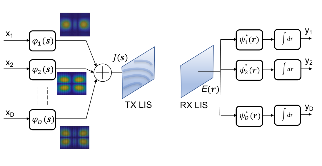
In terms of communication system representation, the eigenfunction decomposition leads to the optimal communication architecture depicted in Fig. 2. From it we obtain the input-output representation in terms of $D$ parallel channels

being $w_{n}$ the AWGN (AWGN), where the $D$ input data streams $\{x_{n}\}$ are associated to the basis functions $\{\phi_{n}(s)\}$ in $\mathcal{S}_{\text{T}}$ (i.e., current spatial distribution on the transmit surface), and they are recovered at the receiver after the correlation of the received signal ${\bf\it E}({\bf{r}})$ with the corresponding basis functions $\{\it\psi_{n}({\bf{s}})\}$ in $\mathcal{S}_{\text{R}}$. This scheme is information-theoretical optimal.

It is worthwhile to highlight that the capacity gain with respect to the case where $D=1$, for a given SNR (SNR), could be significant. For example, supposing uniform power allocation among the $D$ parallel channels, such gain is

which increases with $D$.

The effect of each polarization direction can be studied separately if the components of ${\bf\it J}({\bf{s}})=J_{x}({\bf{s}})\,{\hat{\bf{u}}_{x}}+J_{y}({\bf{s}})\,{\hat{\bf{u}}_{y}}+J_{z}({\bf{s}})\,{\hat{\bf{u}}_{z}}$ are taken orthogonal. Therefore, without loss of generality, suppose we excite the $x$-component, i.e., ${\bf\it J}({\bf{s}})=J_{x}({\bf{s}})\,{\hat{\bf{u}}_{x}}$. By exploiting the identity (37) in Appendix A and considering the last term of (3), the total normalized (i.e., dimensionless) coupling intensity between intelligent surfaces results

where ${\bf{r}}=(r_{x},r_{y},r_{z})\in\mathcal{S}_{\text{R}}$ and ${\bf{s}}=(s_{x},s_{y},s_{z})\in\mathcal{S}_{\text{T}}$ represent the coordinates of the generic points on the receive and transmit surfaces, respectively.

The notation ${\bf\it G}_{x}(\cdot)$ indicates we consider only the first column of tensor ${\bf\it G}(\cdot)$, corresponding to the contribution caused by an excitation in the $x$-direction. Note that in general the excitation in the $x$-direction might contribute to all directions in the received electric field. The expressions for the other exciting directions are similars with mutual exchange of $x$, $y$ and $z$.

In [44] the approximate solution to the eigenfunction problems valid for two collinear rectangular prisms at distance $d$, oriented along the $z$-axis, of volume $V_{\text{T}}=\Delta x_{\text{T}}\,\Delta y_{\text{T}}\,\Delta z_{\text{T}}$ and $V_{\text{R}}=\Delta x_{\text{R}}\,\Delta y_{\text{R}}\,\Delta z_{\text{R}}$, respectively, is presented. Specifically, the solution holds when the volumes are far apart compared to their sizes, i.e., $d\gg\Delta x_{\text{T}},\Delta y_{\text{T}},\Delta z_{\text{T}},\Delta x_{\text{R}},\Delta y_{\text{R}},\Delta z_{\text{R}}$, which means they are in the (Fraunhofer) far-field region. In this case, the DoF available for communication has been found to be

whereas the total (un-normalized) coupling factor is

Note that the thickness of volumes in the $z$ axis does not affect the DoF but only the coupling intensity.

Incidentally, for very small antennas, i.e., $\Delta x_{\text{T}}\Delta x_{\text{R}}\ll\lambda\,d$, $\Delta y_{\text{T}}\Delta y_{\text{R}}\ll\lambda\,d$, only one solution to the eigenfunction problems exists, corresponding to a plane wave that travels with direction from the transmit antenna to the receive antenna. Unfortunately, the result above by [44] is no longer valid when analyzing a LIS as the assumption of far apart antennas, and hence the parallax approximation typical of the Fraunhofer region, does not hold anymore.

The analytical derivation of the eigenfunctions and eigenvalues is in general elusive and one has to resort to e.m. simulations, which could be prohibitive for LIS and typically they do not provide general insights. In the next sections we bypass the direct derivation of the solutions to the eigenfunction problems by resorting to geometric arguments, with the purpose to determine the spatial DoF available for communication. Our aim is to derive simple expressions for particular geometric configurations of interest, also valid in the radiating near-field.

For parallel intelligent surfaces, a way to compute (27) is to approximate the curve delimiting the area $\left[{\bf{k}}({\bf{r}},{\bf{s}})\right]_{{\bf{s}}\in\mathcal{S}_{\text{T}}}$ with a quadrilateral having vertices given by $k_{x}^{(i)}({\bf{r}})=k_{x}\left({\bf{r}},{\bf{s}}^{(i)}\right)$, $k_{y}^{(i)}({\bf{r}})=k_{y}\left({\bf{r}},{\bf{s}}^{(i)}\right)$, $i=1,2,\ldots,5$, with ${\bf{s}}^{(1)}=(x_{0}-L_{\text{x}}/2,y_{0}-L_{\text{y}}/2,d)$, ${\bf{s}}^{(2)}=(x_{0}+L_{\text{x}}/2,y_{0}-L_{\text{y}}/2,d)$, ${\bf{s}}^{(3)}=(x_{0}-L_{\text{x}}/2,y_{0}+L_{\text{y}}/2,d)$, ${\bf{s}}^{(4)}=(x_{0}+L_{\text{x}}/2,y_{0}+L_{\text{y}}/2,d)$, ${\bf{s}}^{(5)}={\bf{s}}^{(1)}$, and then by applying the Gauss’ formula

From (27), (28) and (29) it follows that

Unfortunately, (30) does not admit a closed-form expression in general. However, even though it requires the evaluation of a two-folded integral, its numerical computation is very fast and it does not pose any particular issue compared to the numerical complexity of the eigenfunction problems (8) and (9).

Nevertheless, it could be of interest to derive closed-form expressions of (30) for some significant cases. Specifically, since $L_{\text{x}},L_{\text{y}}\ll d$, setting $x_{0}=y_{0}=0$, (30) gives (details are reported in Appendix B)

For $d\gg S_{\text{x}},S_{\text{y}}$, i.e., in the far-field region, it is

which gives (17) derived in [44].

The limit of (31) for $S_{\text{x}},S_{\text{y}}\rightarrow\infty$, i.e., very large surfaces, is

Equation (33) indicates that the maximum DoF depends only on the area of the transmit surface (normalized to the square half-wavelength), i.e., the area of the smallest of the 2 antennas, and it represents the ultimate DoF limit which is independent of the distance. This result is reminiscent of the DoF in MIMO systems when the channel matrix is full rank, i.e., in the presence of rich multipath [5]. Unfortunately, in LOS channel condition, the rank of the MIMO channel matrix is 1, and hence $D=1$ (only beamforming gain is present). Instead, result (31) indicates that with a LIS one can obtain DoF larger than 1 even in LOS. Having large DoF in LOS could significantly increase the link capacity according to (15), especially at millimeter waves or in the THz band where the multipath is not rich or could be dominated by the LOS component.

Consider now a transmit surface along the plane $xz$ with coordinates ${\bf{s}}=(s_{x},y_{0},s_{z})\in\mathcal{S}_{\text{T}}$ and a perpendicular receive LIS at distance $d$ with coordinates ${\bf{r}}=(r_{x},r_{y},0)\in\mathcal{S}_{\text{R}}$. The centers and sizes of the transmit and receive intelligent surfaces are, respectively, ${\bf{s}}_{0}=(x_{0},y_{0},d)$, $(L_{\text{x}},L_{\text{z}})$ and $(0,0,0)$, $(S_{\text{x}},S_{\text{y}})$. The corresponding areas are $A_{\text{T}}=L_{\text{x}}\,L_{\text{z}}$ and $A_{\text{R}}=S_{\text{x}}\,S_{\text{y}}$.

Following a similar approach as in Sec. IV-A, by setting ${\bf{s}}^{(1)}=(x_{0}-L_{\text{x}}/2,y_{0},d-L_{\text{z}}/2)$, ${\bf{s}}^{(2)}=(x_{0}+L_{\text{x}}/2,y_{0},d-L_{\text{z}}/2)$, ${\bf{s}}^{(3)}=(x_{0}-L_{\text{x}}/2,y_{0},d+L_{\text{z}}/2)$, ${\bf{s}}^{(4)}=(x_{0}+L_{\text{x}}/2,y_{0},d+L_{\text{z}}/2)$, it is

For $d\gg S_{\text{x}},S_{\text{y}}$ one gets

which, compared to (32) valid for parallel surfaces, denotes a dependence on the ratio $S_{\text{y}}/d$. Such a term contributes to increase the DoF when the LIS is tall and hence is capable to “see” better the transmit surface lying on the horizontal plane.

The limit of (34) for $S_{\text{x}},S_{\text{y}}\rightarrow\infty$, i.e., very large surface, is

that is, the same as parallel surfaces.

References

- [1] S. Vitturi, C. Zunino, and T. Sauter, “Industrial communication systems and their future challenges: Next-generation ethernet, IIoT, and 5G,” Proceedings of the IEEE, vol. 107, no. 6, pp. 944–961, June 2019.
- [2] Z. Zhang, Y. Xiao, Z. Ma, M. Xiao, Z. Ding, X. Lei, G. K. Karagiannidis, and P. Fan, “6G wireless networks: Vision, requirements, architecture, and key technologies,” IEEE Vehicular Technology Magazine, vol. 14, no. 3, pp. 28–41, Sep. 2019.
- [3] E. Björnson, L. Sanguinetti, H. Wymeersch, J. Hoydis, and T. L. Marzetta, “Massive MIMO is a reality - what is next?: Five promising research directions for antenna arrays,” Digital Signal Processing, 2019. [Online]. Available: http://www.sciencedirect.com/science/article/pii/S1051200419300776
- [4] T. S. Rappaport, Y. Xing, O. Kanhere, S. Ju, A. Madanayake, S. Mandal, A. Alkhateeb, and G. C. Trichopoulos, “Wireless communications and applications above 100 GHz: Opportunities and challenges for 6G and beyond,” IEEE Access, vol. 7, pp. 78 729–78 757, 2019.
- [5] D. Tse and P. Viswanath, Fundamentals of Wireless Communications. New York, NY: Cambridge University Press, 2005.
- [6] C. L. Holloway, E. F. Kuester, J. A. Gordon, J. O’Hara, J. Booth, and D. R. Smith, “An overview of the theory and applications of metasurfaces: The two-dimensional equivalents of metamaterials,” IEEE Antennas and Propagation Magazine, vol. 54, no. 2, pp. 10–35, April 2012.
- [7] S. B. Glybovski, S. A. Tretyakov, P. A. Belov, Y. S. Kivshar, and C. R. Simovski, “Metasurfaces: From microwaves to visible,” Physics Reports, vol. 634, pp. 1 – 72, 2016. [Online]. Available: http://www.sciencedirect.com/science/article/pii/S0370157316300618
- [8] I. A. Buriak, V. O. Zhurba, G. S. Vorobjov, V. R. Kulizhko, O. K. Kononov, and O. Rybalko, “Metamaterials: Theory, classification and application strategies (review),” Journal of Nano- and Electronic Physics, vol. 8, no. 4, 2016. [Online]. Available: https://search.proquest.com/docview/1853386963?accountid=9652
- [9] L. Di Palma, A. Clemente, L. Dussopt, R. Sauleau, P. Potier, and P. Pouliguen, “Circularly-polarized reconfigurable transmitarray in Ka-band with beam scanning and polarization switching capabilities,” IEEE Transactions on Antennas and Propagation, vol. 65, no. 2, pp. 529–540, Feb 2017.
- [10] Y. Ra’di, V. S. Asadchy, and S. A. Tretyakov, “Tailoring reflections from thin composite metamirrors,” IEEE Transactions on Antennas and Propagation, vol. 62, no. 7, pp. 3749–3760, July 2014.
- [11] V. S. Asadchy, M. Albooyeh, S. N. Tcvetkova, A. Díaz-Rubio, Y. Ra’di, and S. A. Tretyakov, “Perfect control of reflection and refraction using spatially dispersive metasurfaces,” Phys. Rev. B, vol. 94, p. 075142, Aug 2016. [Online]. Available: https://link.aps.org/doi/10.1103/PhysRevB.94.075142
- [12] V. S. Asadchy, Y. Ra’di, J. Vehmas, and S. A. Tretyakov, “Functional metamirrors using bianisotropic elements,” Phys. Rev. Lett., vol. 114, p. 095503, Mar 2015. [Online]. Available: https://link.aps.org/doi/10.1103/PhysRevLett.114.095503
- [13] S. V. Hum and J. Perruisseau-Carrier, “Reconfigurable reflectarrays and array lenses for dynamic antenna beam control: A review,” IEEE Transactions on Antennas and Propagation, vol. 62, no. 1, pp. 183–198, Jan 2014.
- [14] P. Nayeri, F. Yang, and A. Z. Elsherbeni, “Beam-scanning reflectarray antennas: A technical overview and state of the art.” IEEE Antennas and Propagation Magazine, vol. 57, no. 4, pp. 32–47, Aug 2015.
- [15] D. Dardari and D. Massari, “Using MetaPrisms for Performance Improvement in Wireless Communications,” arXiv e-prints, p. arXiv:2003.13505, Mar. 2020.
- [16] J. Hunt, J. Gollub, T. Driscoll, G. Lipworth, A. Mrozack, M. S. Reynolds, D. J. Brady, and D. R. Smith, “Metamaterial microwave holographic imaging system,” J. Opt. Soc. Am. A, vol. 31, no. 10, pp. 2109–2119, Oct 2014. [Online]. Available: http://josaa.osa.org/abstract.cfm?URI=josaa-31-10-2109
- [17] A. Silva, F. Monticone, G. Castaldi, V. Galdi, A. Alù, and N. Engheta, “Performing mathematical operations with metamaterials,” Science, vol. 343, no. 6167, pp. 160–163, 2014. [Online]. Available: https://science.sciencemag.org/content/343/6167/160
- [18] P. Nepa and A. Buffi, “Near-field-focused microwave antennas: Near-field shaping and implementation.” IEEE Antennas and Propagation Magazine, vol. 59, no. 3, pp. 42–53, June 2017.
- [19] D. González-Ovejero, G. Minatti, G. Chattopadhyay, and S. Maci, “Multibeam by metasurface antennas,” IEEE Transactions on Antennas and Propagation, vol. 65, no. 6, pp. 2923–2930, 2017.
- [20] N. Shlezinger, O. Dicker, Y. C. Eldar, I. Yoo, M. F. Imani, and D. R. Smith, “Dynamic metasurface antennas for uplink massive MIMO systems,” IEEE Transactions on Communications, vol. 67, no. 10, pp. 6829–6843, 2019.
- [21] C. Liaskos, S. Nie, A. Tsioliaridou, A. Pitsillides, S. Ioannidis, and I. Akyildiz, “A new wireless communication paradigm through software-controlled metasurfaces,” IEEE Communications Magazine, vol. 56, no. 9, pp. 162–169, Sep. 2018.
- [22] M. Di Renzo and J. Song, “Reflection probability in wireless networks with metasurface-coated environmental objects: an approach based on random spatial processes,” EURASIP Journal on Wireless Communications and Networking, vol. 2019, no. 1, p. 99, Apr 2019. [Online]. Available: https://doi.org/10.1186/s13638-019-1403-7
- [23] M. D. Renzo, M. Debbah, D.-T. Phan-Huy, A. Zappone, M.-S. Alouini, C. Yuen, V. Sciancalepore, G. C. Alexandropoulos, J. Hoydis, H. Gacanin, J. d. Rosny, A. Bounceur, G. Lerosey, and M. Fink, “Smart radio environments empowered by reconfigurable AI meta-surfaces: an idea whose time has come,” EURASIP Journal on Wireless Communications and Networking, vol. 2019, no. 1, p. 129, 2019. [Online]. Available: https://doi.org/10.1186/s13638-019-1438-9
- [24] Y. Yang, S. Zhang, and R. Zhang, “IRS-enhanced OFDMA: Joint resource allocation and passive beamforming optimization,” IEEE Wireless Communications Letters, pp. 1–1, 2020.
- [25] S. Zhang and R. Zhang, “Capacity Characterization for Intelligent Reflecting Surface Aided MIMO Communication,” arXiv e-prints, p. arXiv:1910.01573, Oct. 2019.
- [26] Ö. Özdogan, E. Björnson, and E. G. Larsson, “Using Intelligent Reflecting Surfaces for Rank Improvement in MIMO Communications,” arXiv e-prints, p. arXiv:2002.02182, Feb. 2020.
- [27] K. Ntontin, M. Di Renzo, J. Song, F. Lazarakis, J. de Rosny, D. T. Phan-Huy, O. Simeone, R. Zhang, M. Debbah, G. Lerosey, M. Fink, S. Tretyakov, and S. Shamai, “Reconfigurable Intelligent Surfaces vs. Relaying: Differences, Similarities, and Performance Comparison,” arXiv e-prints, p. arXiv:1908.08747, Aug 2019.
- [28] J. Ye, S. Guo, and M.-S. Alouini, “Joint Reflecting and Precoding Designs for SER Minimization in Reconfigurable Intelligent Surfaces Assisted MIMO Systems,” arXiv e-prints, p. arXiv:1906.11466, Jun. 2019.
- [29] M. Jung, W. Saad, M. Debbah, and C. S. Hong, “On the Optimality of Reconfigurable Intelligent Surfaces (RISs): Passive Beamforming, Modulation, and Resource Allocation,” arXiv e-prints, p. arXiv:1910.00968, Oct 2019.
- [30] S. Hu, F. Rusek, and O. Edfors, “Beyond massive MIMO: The potential of data transmission with large intelligent surfaces,” IEEE Transactions on Signal Processing, vol. 66, no. 10, pp. 2746–2758, May 2018.
- [31] F. Guidi and D. Dardari, “Radio Positioning with EM Processing of the Spherical Wavefront,” arXiv e-prints, p. arXiv:1912.13331, Dec. 2019.
- [32] O. M. Bucci and G. Franceschetti, “On the degrees of freedom of scattered fields,” IEEE Transactions on Antennas and Propagation, vol. 37, no. 7, pp. 918–926, July 1989.
- [33] M. Franceschetti, M. D. Migliore, and P. Minero, “The capacity of wireless networks: Information-theoretic and physical limits,” IEEE Trans. Inf. Theor., vol. 55, no. 8, pp. 3413–3424, Aug. 2009. [Online]. Available: http://dx.doi.org/10.1109/TIT.2009.2023705
- [34] M. Franceschetti, M. D. Migliore, P. Minero, and F. Schettino, “The degrees of freedom of wireless networks via cut-set integrals,” IEEE Transactions on Information Theory, vol. 57, no. 5, pp. 3067–3079, May 2011.
- [35] M. Franceschetti, Wave Theory of Information. Cambridge, UK: Cambridge University press, 2018.
- [36] A. Pizzo, T. L. Marzetta, and L. Sanguinetti, “Spatially-Stationary Model for Holographic MIMO Small-Scale Fading,” arXiv e-prints, p. arXiv:1911.04853, Nov. 2019.
- [37] ——, “Degrees of Freedom of Holographic MIMO Channels,” arXiv e-prints, p. arXiv:1911.07516, Nov. 2019.
- [38] R. F. Harrington, Time-Harmonic Electromagnetic Fields. New York, USA: IEEE Press - Wiley, 2001.
- [39] S. Hu, K. Chitti, F. Rusek, and O. Edfors, “User assignment with distributed large intelligent surface (LIS) systems,” in 2018 IEEE 29th Annual International Symposium on Personal, Indoor and Mobile Radio Communications (PIMRC), Sep. 2018, pp. 1–6.
- [40] A. Amiri, M. Angjelichinoski, E. de Carvalho, and R. W. Heath, “Extremely large aperture massive MIMO: Low complexity receiver architectures,” in 2018 IEEE Globecom Workshops (GC Wkshps), Dec 2018, pp. 1–6.
- [41] M. Jung, W. Saad, Y. Jang, G. Kong, and S. Choi, “Reliability analysis of large intelligent surfaces (LISs): Rate distribution and outage probability,” IEEE Wireless Communications Letters, vol. 8, no. 6, pp. 1662–1666, 2019.
- [42] ——, “Performance analysis of large intelligent surfaces (LISs): Asymptotic data rate and channel hardening effects,” IEEE Transactions on Wireless Communications, vol. 19, no. 3, pp. 2052–2065, 2020.
- [43] L. Zhang, X. Q. Chen, S. Liu, Q. Zhang, J. Zhao, J. Y. Dai, G. D. Bai, X. Wan, Q. Cheng, G. Castaldi, V. Galdi, and T. J. Cui, “Space-time-coding digital metasurfaces,” Nature Communications, vol. 9, no. 1, p. 4334, 2018. [Online]. Available: https://doi.org/10.1038/s41467-018-06802-0
- [44] D. A. B. Miller, “Communicating with waves between volumes: evaluating orthogonal spatial channels and limits on coupling strengths,” Appl. Opt., vol. 39, no. 11, pp. 1681–1699, Apr 2000. [Online]. Available: http://ao.osa.org/abstract.cfm?URI=ao-39-11-1681
- [45] R. Piestun and D. A. B. Miller, “Electromagnetic degrees of freedom of an optical system,” J. Opt. Soc. Am. A, vol. 17, no. 5, pp. 892–902, May 2000. [Online]. Available: http://josaa.osa.org/abstract.cfm?URI=josaa-17-5-892
- [46] D. Dardari, “Communicating with intelligent surfaces,” in 2020 IEEE International Conference on Communications (ICC): Communication Theory Symposium (IEEE ICC’20 - CT Symposium), Dublin, Ireland, Jun. 2020.
- [47] C. A. Balanis, Antenna Theory: analysis and design. New Jersey, USA: Wiley, 2016.
- [48] A. S. Y. Poon, R. W. Brodersen, and D. N. C. Tse, “Degrees of freedom in multiple-antenna channels: a signal space approach,” IEEE Transactions on Information Theory, vol. 51, no. 2, pp. 523–536, Feb 2005.
- [49] D. A. B. Miller, “Waves, modes, communications, and optics: a tutorial,” Adv. Opt. Photon., vol. 11, no. 3, pp. 679–825, Sep 2019. [Online]. Available: http://aop.osa.org/abstract.cfm?URI=aop-11-3-679
- [50] D. Slepian, “Some comments on Fourier analysis, uncertainty and modeling,” SIAM Review, vol. 25, no. 3, pp. 379–393, 1983. [Online]. Available: https://doi.org/10.1137/1025078