Fast Deflation Sparse Principal Component Analysis
via Subspace Projections

We first introduce the deflation in the context of PCA. Let $X\in\mathbb{R}^{n\times d}$ be a data matrix encoding $n$ samples and $d$ variables. Without loss of generality, we assume that the variables contained in the columns of $X$ are centered. Let $A_{0}=X^{T}X\in\mathbb{R}^{d\times d}$ denote the sample covariance matrix.

Deflation method aims to find $r$ principal components by solving the following optimization problem sequentially:

for $t=1,2,\ldots,r$. The matrix $A_{t}$ should be updated recursively to eliminate the influence of the previous computed loading. For instance, a widely used deflation formula is

Note that the size of $A_{t}$ is fixed as $d\times d$ in each round, which brings up a heavy cumulative workload in high dimensions. In Section 3, we shall introduce some subspace projections to alleviate this problem.

Given a principal component $\mathbf{z}=(z_{1},\ldots,z_{d})^{T}\in\mathbb{R}^{d}$, it is a common way to employ an additional truncation operation to ensure sparsity [16, 25, 31]. In this paper, we will use the truncation operator $\mathcal{T}_{\lambda}(\cdot):\mathbb{R}^{d}\rightarrow\mathbb{R}^{d}$, which is one of the following three types.

• •

  $\mathcal{T}_{S}$ (Truncation by Sparsity). Given a cardinality $0<\kappa_{S}<d$, truncate the smallest $\kappa_{S}$ entries according to their absolute values. The main advantage of $\mathcal{T}_{S}$ lies in its direct control of sparsity.

• •

  $\mathcal{T}_{E}$ (Truncation by Energy). Sort the entries of $\mathbf{z}$ in ascending order such that $|\bar{z}_{1}|\leq|\bar{z}_{2}|\leq\ldots\leq|\bar{z}_{d}|$. For a given real number $0<\kappa_{E}<1$, choose $i^{*}=\max\{i\}$ with $i$ satisfying $\sum_{j=1}^{i}\bar{z}_{j}^{2}\leq\kappa_{E}\|\mathbf{z}\|^{2}$. Then truncate the smallest $i^{*}$ entries, whose energy accounts for at most $\kappa_{E}$ proportion,

• •

  $\mathcal{T}_{H}$ (Hard-Threshholding). Given a threshold $\kappa_{H}>0$, set $\mathcal{T}_{H}(z_{i})=0$ if $|z_{i}|<\kappa_{H}$, and $\mathcal{T}_{H}(z_{i})=z_{i}$ otherwise.

For any $\mathbf{z}\in\mathbb{R}^{d}$, denote by $s(\mathbf{z})=1-\|\mathbf{z}\|_{0}/d$ its sparsity. For $\mathcal{T}_{S}$, it is trivial that $\kappa_{S}/d\leq s(\mathbf{z})<1$. For $\mathcal{T}_{E}$, it was proved in [16] that

For $\mathcal{T}_{H}$, it was proved in [16] that

Therefore, the truncation parameter can be used to control the sparsity of the loadings.

For $t=1,2,\ldots,r$, we aim to find $\alpha_{t}$ sequentially such that

where $\{P_{t-1}\in\mathbb{R}^{d\times m}\}_{t=1}^{r}$, $m<\min\{n,d\}$, are subspace projections to be determined later. In many practical fields, such as genomic analysis, one can choose $m\ll d$ to greatly save the computational cost.

It is observable that the vector $P_{t-1}\alpha_{t}$, which belongs to the subspace spanned by the columns of the matrix $P_{t-1}$, is an approximation of principal component $z_{t}$ in (1). From the view point of rank-1 approximation, (5) is identical to the following constrained optimization problem

In order to achieve a sparse loading, one could post process $P_{t-1}\alpha_{t}$ by use of a truncation operation. Specifically, for a given truncation operator $\mathcal{T}_{\lambda}$, let

be the corresponding sparse loading. It should be noticed that the truncation parameter $\lambda$ is a tuning parameter, similar as the penalty weight in the penalized approaches.

It is worth emphasizing that the key difference between our SPCA-SP from most existing SPCA methods, e.g. [16, 21, 25, 31], is the introduction of an additional subspace projection in each round, which intends to make the computation of each loading restricted in a low dimensional space, and at the same time ensures the orthogonality of all sparse loadings.

Another noteworthy point is that SPCA-SP is a postprocessing based algorithm without using sparsity penalization. Sparsity penalized method is more commonly used in literature due to its distinct mathematical background . But it seems impossible to apply such technique here, because $P_{t-1}$ is not invertible and thus commonly used block gradient descent technique [30] can not solve the corresponding optimization objective.

In this section, we will introduce the construction of subspace projections in detail. We shall use the randomized SVD algorithm to construct an initial projection, just like fast PCA [1]. After then, we will employ a sequence of QR factorization to build the other subspace projections. The related construction process is very technical. It is worth to emphasize that the subspaces determined by these projections are orthogonal to the previously found sparse loadings. It is well known that PCA loadings are orthogonal, but as pointed out by [16, 25], this property is easily lost in SPCA. Orthogonality is significant in SPCA because it ensures the independence of the physical meaning of the loadings, thus further simplifying the interpretation.

Firstly, we turn to a fast SVD algorithm, named as LinearTimeSVD [8], to construct the projection $P_{0}$. The purpose of using this algorithm is to alleviate a part of time consuming. If $n$ or $d$ is not too large, exact SVD can also be used to construct the initial projection $P_{0}$.

For a given data matrix $X\in\mathbb{R}^{n\times d}$, we generate a probability sequence as follows

where $\mathbf{x}_{(i)}$ denotes the $i$-th row of $X$. Let $c$ be an integer satisfying $c\leq\min\{n,d\}$. For $t=1,\ldots,c$ , sample $i_{t}\in\{1,\ldots,n\}$ with $\textbf{Pr}[i_{t}=\tau]=\xi_{i},\>\tau=1,\ldots,n$. Let $X_{c}$ be a matrix of size $c\times d$, the $t$-th row of which is determined by $\mathbf{x}_{c,(t)}=\mathbf{x}_{(i_{t})}/\sqrt{c\xi_{i_{t}}}$, $t=1,\ldots,c$. The singular value decomposition of $X_{c}X_{c}^{T}$ is denoted by

where $\sigma_{1}\geq\cdots\geq\sigma_{c}>0$ are singular values of $X_{c}$ and $[\mathbf{u}_{1},\ldots,\mathbf{u}_{c}]$ forms an orthogonal matrix of size $c\times c$. Choosing $m\leq c$, let

The initial projection $P_{0}$ is then defined by

According to [8], the time complexity of the construction of $P_{0}$ is $O(nd+c^{2}d+c^{3})$.

The sample size $c$ and the subspace dimension $m$ are free parameters. For an expected cumulative percentage of explained variance $0<\texttt{CPEV}<1$, one shall choose $c$ and $m$ to satisfy

where $\mathbf{Tr}$ denotes the matrix trace. This is not a difficult task when we are only interested in a few leading principal components.

Next, we are to construct the subspace projections $P_{t}$, $t\geq 1$ in a sequent manner, based on the calculated sparse loadings. We will employ QR factorization [29] in the construction process. QR factorization decomposes the input matrix into the product of a square, orthogonal matrix $Q$ and an upper triangular matrix $R$. It is usually used in solving linear systems of equations. The QR decomposition of a matrix can be computed in different ways. The use of Givens Rotations [10] and Householder reflections [14] are two most commonly used and best known ones. Here we prefer to use Householder version because it will be more efficient for the decomposition object defined below.

For any given matrix $A\in\mathbb{R}^{n\times m}$, a sequence of Householder reflections [14] can be used to zero-out all the coefficients below the diagonal to compute its QR factorization:

Each transformation $H_{k}$ annihilates the coefficients below the diagonal of column $k$ and modifies the coefficients in the trailing submatrix $A(k:n,k+1:m)$.

Without loss of generality, suppose that we have constructed the projection matrix $P_{t-1}$, $\forall t\geq 1$, and obtained the corresponding sparse loadings $\tilde{\mathbf{z}}_{1},\ldots,\tilde{\mathbf{z}}_{t}$. To formulate the subsequent projection $P_{t}$, we introduce an auxiliary compound matrix as follows:

Applying Household QR factorization to the matrix $B_{t}$ yields $B_{t}=QR$, where $Q=[\mathbf{q}_{1},\ldots,\mathbf{q}_{d}]\in\mathbb{R}^{d\times d}$ is an orthogonal matrix. Consequently, the new subspace projection $P_{t}\in\mathbb{R}^{d\times m}$ is constituted from a submatrix of $Q$, i.e.,

Noting that $Q^{T}B_{t}=R$ and $R$ is an upper triangular matrix, we immediately have

The above property is desirable because it means that the search space for the $(t+1)$-th untruncated loading is orthogonal to all previously computed sparse loadings. Therefore, we can anticipate that after small truncation, the sparse loadings are close to orthogonal. This makes interpretation simpler.

In this section, we give a theoretical result about the connection between orthogonality and sparsity after three truncation operations. As far as we know, this relationship has never been revealed before.

First we introduce a notation to measure the orthogonality of two vectors. Define

Observe that a larger $\langle\mathbf{a},\mathbf{b}\rangle$ means a better orthogonality.

The following lemma gives an upper bound of the orthogonality of two vectors after truncation.

The next proposition gives the relationship between sparsity and orthogonality after applying the truncation operators introduced in Section 2.2.

In view of Proposition 3.2 and (11), we can use truncation parameters to control the orthogonality performance of the sparse loadings.

In this section, we test whether SPCA-SP can recover some underlying sparse loadings of the synthetic data introduced in [32], which include three hidden Gaussian factors

Then 10 observable variables are generated by

We consider $r=2$ since the first two principal components together explain 99.6% of the total variance. Note that $h_{1}$ and $h_{2}$ are independent, while $h_{3}$ is correlated with both of them but more dependent on $h_{2}$. The most acceptable two sparse loading patterns are $1-4$, $9-10$; $5-10$ and $1-4$; $5-10$.

We take $c=5$ and $m=3$ as an example. The computed sparse loadings based on three types of truncation operations are listed in Table 4.1. It is obvious that SPCA-SP successfully recovers the desirable sparse loading patterns.

Pitprops data, which contains 180 observations and 13 features, is a standard benchmark to evaluate the performance of SPCA algorithms. The first six principal components explain 86.9% variance of the data. The algorithms are tested to find $r=6$ sparse loadings. We directly cite the best results reported in [16] for the baseline algorithms. Set $c=11$ and $m=5$. The truncation parameters in SPCA-SP are tuned to yield the expected loading patterns.

It is observed from Table 4.2 that SPCA-SP has achieved the competitive empirical performance with these baseline algorithms. Especially, in the case of balanced loading pattern 3-3-3-3-3-3, SPCA-SP ($\mathcal{T}_{S},\kappa_{S}=10$) obtains the maximum explained variance, while its orthogonality is better than that of all other algorithms except SPCA. Furthermore, SPCA-SP ($\mathcal{T}_{H},\kappa_{H}=0.4$) outperforms classical SPCA under a more sparse loading mode.

In this section, we consider high-dimensional Gene data [11], which contains 72 samples with 7129 variables, Since $n\ll d$, we use an exact SVD algorithm to generate the initial subspace projection for SPCA-SP.

We first examine how the performance of SPCA-SP is affected by the subspace dimension when $2\leq m\leq 72$. For simplicity, we fix truncation parameters as $\kappa_{S}=5500$, $\kappa_{E}=0.01$ and $\kappa_{H}=1/300$. As shown in Figure 1, when $m$ increases from 2 to 6, explained variance, sparsity and orthogonality all increase rapidly. After then the performance on three criteria becomes stable, almost unchanged. On the other hand, the time cost goes approximately linearly with the subspace dimension. These observations demonstrate that SPCA-SP is robust and stable with respect to the subspace dimension $m$. The observation results also show that in practical application, a proper small $m$ is enough to ensure a good tradeoff between explained variance, sparsity, orthogonality and computational speed.

Next, we choose Tpower and SPCArt algorithms as our comparison objects. As shown in [16, 31], both methods are among the top fast SPCA solvers. Specifically, Tpower is an iterative power method along with $\mathcal{T}_{S}$ truncation, while SPCArt belongs to a block method alternatively rotating the PCA basis and truncating small entries.

We run the algorithms on a range of truncation parameters. The subspace dimension in SPCA-SP is kept as $m=6$. The results of CPEV, orthogonality and computational time under the same sparsity are depicted in Figure 2. It is obvious from Figure 2 (a) and (b) that Tpower, SPCArt and SPCA-SP perform similarly on explained variance and orthogonality. But from Figure 2 (c), one can find that only the time consuming of SPCA-SP is stable with respect to sparsity. Furthermore, due to the introduction of subspace projections, our SPCA-SP method achieves the best performance on the computational speed as expected.

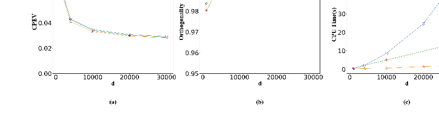
In this section, we consider random data sets with increasing dimensions. As in [16, 21], we first consider zero-mean, unit variance Gaussian data with $d=100,400,700,1000,1300$, and take $n=d+1$. We still compare SPCA-SP with Tpower and SPCArt methods. For simplicity, we use the truncation $\mathcal{T}_{S}$ for three methods. Once the truncation parameter $\kappa_{S}$ is fixed, all three methods have the same sparsity. We take $r=20$ and $\kappa_{S}=[0.7d]$ as an example. In SPCA-SP, let $c=d/2$ and $m=80$. It is observed from Figure 3 that the performance of all three methods are similar on explained variance and orthogonality. But, as reflected in Figure 3 (c), the time cost of Tpower and SPCArt increases nonlinearly with the data dimension, while that of SPCA-SP is lower and goes almost linearly.

Next we consider an extra high-dimensional case with $n\ll d$. We fix $n=500$ and consider zero-mean, unit variance Gaussian data with $d=1000,4000,10000,20000,30000$. An exact SVD algorithm is employed to yield the initial subspace projection. The subspace dimension is fixed as $m=30$. We take $r=20$ and $\kappa_{S}=[0.85d]$ as an example. From Figure (4), we find the time consuming of SPCA-SP for such extra high-dimensional data is much lower as compared to Tpower and SPCArt.

The results from Figure 3 and Figure 4 demonstrate that our SPCA-SP is highly efficient in processing high-dimensional data.

References

- [1] G. Abraham, M. Inouye, Fast principal component analysis of large-scalegenome-wide data. PLoS One, 9(4):1-5, 2014.
- [2] Y. Aitsahalia, D. Xiu, Principal component analysis of high frequency data. J. Am. Stat. Assoc., 114:287-303, 2019.
- [3] T. Bouwmans, E. Zahzah, Robust PCA via principal component pursuit: a review for a comparative evaluation in video surveillance. Comput. Vis. Image Underst. 122:22-34, 2014.
- [4] R. Bro, A.K. Smilde, Principal component analysis. Analytical Methods, 6:2812-2831, 2014.
- [5] A. d’Aspremont, L.El Ghaoui, M.I. Jordan, G. Lanckriet, A direct formulation for sparse PCA using semidefinite programming. SIAM Rev., 49:434-448, 2007.
- [6] I.S. Dhindsa, R. Agarwal, H.S. Ryait, Principal component analysis-based muscle identification for myoelectric-controlled exoskeleton knee. J. Appl. Stat., 44:1707-1720, 2017
- [7] A. d’Aspremont, F. Bach, L.El Ghaoui, Full regularization path for sparse principal component analysis. Proceedings of the 24th International Conference on Machine Learning, 177-184, 2007.
- [8] P. Drineas, R. Kannan, M.W. Mahoney, Fast monte carlo algorithms for matrices ii:computing a low-rank approximation to a matrix. SIAM J. Comput., 36:158-183, 2006.
- [9] Fukuda, Kosei, Principal-component-based generalized-least-squares approach for panel data. J Stat. Comput. Sim., 86:874-890, 2016.
- [10] W. Givens, Computation of plane unitary rotations transforming a general matrix to triangular form. Journal of the Society for Industrial and Applied Mathematics, 6:26-50, 1958.
- [11] T.R. Golub, D.K. Slonim, P. Tamayo, et al., Molecular classification of cancer: class discovery and class prediction by gene expression monitoring. Science, 286:531-537, 1999.
- [12] N. Halko, P.G. Martinsson, Y. Shkolnisky, M. Tygert An algorithm for the principal component analysis of large data sets. SIAM J. Sci. Comput., 33:2580-2594, 2011.
- [13] A. Hannachi, I.T. Jolliffe, D.B. Stephenson, N. Trendafilov, In search of simple structures in climate: simplifying EOFs. Int. J. Climatol. 26:7-28, 2006.
- [14] S. Householder, Unitary triangularization of a nonsymmetric matrix, J. Assoc. Comput. Mach, 5:339-342, 1958.
- [15] K. Hron, A. Menafoglio, M. Templ, K. Hruzova, P. Filzmoser, Simplicial principal component analysis for density functions in bayes spaces. Comput. Statist. Data Anal., 94:330-350, 2016.
- [16] Z. Hu, G. Pan, Y. Wang, Z. Wu, Sparse principal component analysis via rotation and truncation. IEEE Trans. Neur. Net. Lear., 27:875-890, 2016.
- [17] J.N. Jeffers, Two case studies in the application of principal component analysis. Applied Statistics, 16:225-236, 1967.
- [18] I.T. Jolliffe, Principal Component Analysis. New York: Springer-Verlag, 1986.
- [19] I.T. Jolliffe, Rotation of principal components: choice of normalization constraints. J. Appl. Stat., 22:29-35, 1995.
- [20] I.T. Jolliffe, N.T. Trendafilov, M. Uddin, A modified principal component technique based on the LASSO. J. Comput. Graph. Statist., 12:531-547, 2003.
- [21] M. Journee, Y. Nesterov, P. Richtarik, R. Sepulchre, Generalized power method for sparse principal component analysis. J. Mach. Learn. Res., 11:517-553, 2010.
- [22] S. Kawano, H. Fujisawa, T. Takada, T. Shiroishi, Sparse principal component regression with adaptive loading. Comput. Statist. Data Anal., 89:192-203, 2015.
- [23] S. Kawano, H. Fujisawa, T. Takada, T. Shiroishi, Sparse principal component regression for generalized linear models. Comput. Statist. Data Anal., 124:180-196, 2018.
- [24] Z. Ma, Sparse principal component analysis and iterative thresholding. Annals of Statistics, 41:772-801, 2013.
- [25] L. Mackey, Deflation methods for sparse PCA. Advances in NIPS, 21:1017-1024, 2009.
- [26] R.W. Preisendorfer, C.D. Mobley, Principal component analysis in meteorology and oceanography. Amsterdam, The Netherlands: Elsevier, 1988.
- [27] Y. Saad, Projection and deflation method for partial pole assignment in linear state feedback. IEEE Trans. Automat. Contr., 33:290-297, 1988.
- [28] H. Shen, J.Z. Huang, Sparse principal component analysis via regularized low rank matrix approximation. J. Multivariate Anal., 99:1015-1034, 2008.
- [29] L.N. Trefethen, D. Bau, Numerical Linear Algebra. SIAM, Philadelphia, 1997.
- [30] S.J. Wright, Coordinate descent algorithms. Mathematical Programming, 151:3-34, 2015.
- [31] X. Yuan, T. Zhang, Truncated power method for sparse eigenvalue problems. J. Mach. Learn. Res., 14:899-925, 2013.
- [32] H. Zou, T. Hastie, R. Tibshirani, Sparse principal component analysis. J. Comput. Graph. Statist., 15:265-286, 2006.