跳到论文正文
W Papers独立论文阅读器 arXiv:1912.01387 论文正文 计算阅读时间 · 0%
引用这篇论文根据当前论文元数据生成,正式投稿前建议核对。


License: CC BY 4.0
arXiv:1912.01387v2 [q-fin.MF] 15 Feb 2021

Pricing FX Options under Intermediate Currency

S. Maurer Thanks: School of Mathematical Sciences, University of Nottingham, UK; Simon.Maurer@nottingham.ac.uk    T.E. Sharp Thanks: Credit Suisse, Zurich, Switzerland    M.V. Tretyakov Thanks: School of Mathematical Sciences, University of Nottingham, UK; Michael.Tretyakov@nottingham.ac.uk
Abstract

We suggest an intermediate currency approach that allows us to price options on all FX markets simultaneously under the same risk-neutral measure which ensures consistency of FX option prices across all markets. In particular, it is sufficient to calibrate a model to the volatility smile on the domestic market as, due to the consistency of pricing formulas, the model automatically reproduces the correct smile for the inverse pair (the foreign market). We first consider the case of two currencies and then the multi-currency setting. We illustrate the intermediate currency approach by applying it to the Heston and SABR stochastic volatility models, to the model in which exchange rates are described by an extended skewed normal distribution, and also to the model-free approach of option pricing.

Keywords: foreign exchange market, FX option pricing, foreign-domestic symmetry, multi-currency options, skewed normal distribution.

1 Introduction

As it is well known (see e.g. [4, 30] and also Section 2 here), in the case of a foreign exchange (FX) for two currencies (say, GBP and EUR) no measure is simultaneously risk-neutral for the market on which GBP is the domestic currency and for the market on which EUR is the domestic currency. This can be seen as an asymmetry between the different market views due to the different choice of numeraires. In practice currency pair conventions are usually used in order to standardize option price quotations for each specific currency pair [24, 30]. But this can lead to calibration difficulties. Each of the domestic markets has its own volatility smile curve for options on the corresponding foreign currency. Suppose we want to use a stochastic volatility model given under a risk-neutral measure on the GBP domestic market which we calibrate to the smile for options on EUR. If we re-write this model for the inverse pair, i.e., where options on GBP are traded, in a risk-neutral fashion, we need to calibrate it to the smile on this market as the previously found parameters of the model typically do not match the smile for the inverse pair. This is inconvenient. This situation becomes even more complicated in a multi–currency setting while it is of practical importance to be able to price options on the global FX market in a consistent fashion. With a large number NN of currencies, the existence of a consistent FX model is not trivial as a suitable model must preserve relationships between all NN currencies and consistency of volatility smiles between all N⁡(N−1)/2N(N-1)/2 cross pairs.

To address these problems of consistent FX modelling, in [11] (see also [13, 12, 8]) the concept of intrinsic currency [11, 12] or artificial currency [8] was introduced. The approach of [11] is based on the idea that each currency has an ‘intrinsic value’, which is a description of the value of a currency in relation to other currencies. In the intrinsic currency-valuation framework of [11, 12] one models the NN intrinsic values of NN currencies rather than modelling the N−1N-1 exchange rates. In [12] Doust extends his original idea of the intrinsic currency-valuation framework to a SABR-type model, which allows to capture the observed volatility smile on the FX market in a multi-currency setting. On a FX market with NN currencies, he describes the market with NN intrinsic currency values and chooses one (without loss of generality) as the valuation currency and its associated risk–neutral measure, which produces the usual risk–neutral processes for all exchange rates. In [8] NN exchange rates between an artificial currency and NN real currencies are modelled under a risk-neutral measure associated with the artificial currency so that all relationships (in particular, the inversion property that the exchange rate for a pair of real currencies and for their inverse satisfy SDEs of a similar form) between NN currencies are satisfied.

Here we explore a very simple but very valuable from the practical angle idea: find a numeraire with respect to which we can price all FX derivatives traded on any of the domestic markets simultaneously under the same measure. This resolves the issue highlighted above: models for different currency pairs can be calibrated to all smiles in a consistent manner. For instance, in the case of two currencies, it is sufficient to calibrate a model on e.g. the GBP domestic market and the smile on the EUR domestic market is automatically reproduced without any need of additional calibration.

We show that such a numeraire exists via introducing the concept of an intermediate pseudo-currency. The main difference with [11, 13, 12, 8] is that the pseudo-currency is explicitly defined via exchange rates of real currencies, while in [11, 13, 12, 8] exchange rates of real currencies are described via an artificial, not observed currency. Consequently, we naturally model N−1N-1 exchange rates, not NN as in [11, 13, 12, 8]. Further, we can use three modelling approaches in a consistent manner. The first one is the traditional modelling way in Financial Mathematics, where we start from a stochastic model for N−1N-1 exchange rates under a ‘market’ measure and then we introduce a pseudo-currency market which, as we show, has a risk-neutral measure. Under this risk-neutral measure (the intermediate pseudo-currency is used as the numeraire) we can price FX products on all currency markets simultaneously which guarantees consistency of volatility smiles and other natural relationships between currencies (e.g., the foreign-domestic symmetry). This approach allows us to start with popular stochastic volatility models (e.g., Heston or SABR) written under a ‘market’ measure and derive the corresponding consistent models on the pseudo-currency market. Alternatively, in the second approach, from the start we model exchange rates under a risk-neutral measure or under a forward measure associated with the pseudo-currency market. The third approach is model-free (see [1, 15, 2, 9] and references therein), where we reconstruct a risk-neutral measure or a forward measure from volatility smiles. We note that the intermediate pseudo-currency in comparison with the intrinsic currency of [11] does not have a financial interpretation, but our focus here is solely on consistent calibration and modelling of exchange rates.

The rest of the paper is organized as follows. In Section 2 we recall that there is no measure which is simultaneously risk-neutral for both domestic and foreign FX markets and also recall the foreign-domestic symmetry. A convenient numeraire and the associated intermediate pseudo-currency market are introduced in Section 3, where the corresponding pricing formulas for FX options are also derived. This is done for clarity of the exposition in the case of a single currency pair. We extend the intermediate pseudo-currency concept to the multi–currency setting in Section 4. In Section 5 we illustrate the concept by first applying it to the Heston model [21] and SABR [20]. Then, for further illustration, we model the spot exchange rate using an extended skewed normal distribution. This exchange rate model is an illustration of how one can describe the observed fat-tailed distribution of the log exchange rate (compared to the log normal assumption). The considered extended skewed normal distribution is constructed by combining one normal and two shifted half-normal distributed random variables and it allows a flexible control of the tails of the spot exchange rate distribution. We note that the use of the extended skewed normal distribution in pricing FX options is somewhat new. Further, we illustrate our FX option pricing mechanism on the model-free approach. We provide some calibration examples in Section 6.

2 Preliminaries

In this section we recall the well-known fact (see e.g. [4, 30]) that there is no measure which is simultaneously risk-neutral for both the domestic and the foreign market. We also state the foreign-domestic symmetry. For definiteness, in this section and in Section 3 we use the EUR-USD and USD-EUR pairs.

Let us recall that the EUR-USD spot exchange rate at time tt

f(t):=S€/$(t)f(t):=S_{\text{€}/\$}(t)

is quoted as

units of USDone EUR,\frac{\text{units of USD}}{\text{one EUR}},

and

S$/€​(t)=1S€/$(t)=1f⁡(t).S_{\$/\text{€}}(t)=\frac{1}{S_{\text{€}/\$}(t)}=\frac{1}{f(t)}.

In currency pairs (e.g. EUR-USD), the first mentioned currency is known as the foreign (or base) currency, while the second is known as the domestic currency (or numeraire) [5, 30].

Within the standard option pricing setting, we assume that the currency market under a ‘market’ measure is described by the system:

d​B$=r$​(t)​B$​d​t,\displaystyle dB_{\$}=r_{\$}(t)B_{\$}dt, (2.1)
d​B€=r€​(t)​B€​d​t,\displaystyle dB_{\text{€}}=r_{\text{€}}(t)B_{\text{€}}dt,
d​f=μ⁡(t)​f​d​t+σ⁡(t)​f​d​W​(t),\displaystyle df=\mu(t)fdt+\sigma(t)fdW(t),

where B$​(t)B_{\$}(t), B€​(t)B_{\text{€}}(t) and r$​(t)r_{\$}(t), r€​(t)r_{\text{€}}(t) are USD and EUR bank accounts with their short interest rates, respectively; σ⁡(t)>0\sigma(t)>0 is a volatility, μ⁡(t)\mu(t) is a drift; and W⁡(t)W(t) is a standard Wiener process. It is assumed that the coefficients r$​(t)r_{\$}(t), r€​(t)r_{\text{€}}(t), σ⁡(t)\sigma(t), and μ⁡(t)\mu(t) are stochastic processes adapted to a filtration ℱt\mathcal{F}_{t} to which W⁡(t)W(t) is also adapted (typically, in stochastic volatility models ℱt\mathcal{F}_{t} is larger than the natural filtration of OPENW⁡(t)),W(t)), and they have bounded second moments. We also require that σ⁡(t)\sigma(t) satisfies Novikov’s condition.

On the USD market, the foreign currency EUR is paid for by USD (the domestic currency) and the risky asset is

Y€/$(t)=S€/$(t)B€(t),Y_{\text{€}/\$}(t)=S_{\text{€}/\$}(t)B_{\text{€}}(t),

while on the EUR market the risky asset is

Y$/€​(t)=S$/€​(t)​B$​(t).Y_{\$/\text{€}}(t)=S_{\$/\text{€}}(t)B_{\$}(t).

Following the classical theory of pricing, we have to find equivalent (local) martingale measures (EMMs) Q$Q^{\$} and Q€Q^{\text{€}} under which the corresponding discounted risky assets are (local) martingales. By standard arguments we arrive at the SDEs for f⁡(t)f(t) and g⁡(t):=1/f⁡(t)g(t):=1/f(t) written under the corresponding EMMs:

d​f\displaystyle df =\displaystyle= (r$​(t)−r€​(t))​f​d​t+σ⁡(t)​f​d​WQ$​(t),\displaystyle(r_{\$}(t)-r_{\text{€}}(t))fdt+\sigma(t)fdW^{Q^{\$}}(t), (2.2)
d​g\displaystyle dg =\displaystyle= (r€​(t)−r$​(t))​g​d​t−σ⁡(t)​g​d​WQ€​(t),\displaystyle(r_{\text{€}}(t)-r_{\$}(t))gdt-\sigma(t)gdW^{Q^{\text{€}}}(t), (2.3)

where WQ$​(t)W^{Q^{\$}}(t) is a standard Wiener process under Q$Q^{\$} and WQ€​(t)W^{Q^{\text{€}}}(t) is a standard Wiener process under Q€Q^{\text{€}}. We can see (cf. (2.1) and (2.2)-(2.3)) that the market prices of risk on the two markets differ:

γ€​(t)=μ⁡(t)+r€​(t)−r$​(t)σ⁡(t)≠σ2​(t)−μ⁡(t)+r$​(t)−r€​(t)−σ⁡(t)=γ$​(t)\gamma_{\text{€}}(t)=\frac{\mu(t)+r_{\text{€}}(t)-r_{\$}(t)}{\sigma(t)}\neq\frac{\sigma^{2}(t)-\mu(t)+r_{\$}(t)-r_{\text{€}}(t)}{-\sigma(t)}=\gamma_{\$}(t)

(recall that OPENσ⁡(t)>0).\sigma(t)>0). Thus,

Q$≠Q€,Q^{\$}\neq Q^{\text{€}}, (2.4)

i.e., there is no measure which is simultaneously risk-neutral for the EUR domestic market and for the USD domestic market in this rather general setting. We remark that (2.4) does not lead to an arbitrage opportunity.

Note that the SDE (2.2) for ff under the measure Q€Q^{\text{€}} takes the form

d​f=(r$​(t)−r€​(t)+σ2​(t))​f​d​t+σ⁡(t)​f​d​WQ€.df=(r_{\$}(t)-r_{\text{€}}(t)+\sigma^{2}(t))fdt+\sigma(t)fdW^{Q^{\text{€}}}. (2.5)

Intuitively, one could think that the drift for the exchange rate g⁡(t)=1/f⁡(t)g(t)=1/f(t) in (2.3) should be the negative of the drift of f⁡(t)f(t) under the same measure, i.e. −(r€​(t)−r$​(t))=r$​(t)−r€​(t)-(r_{\text{€}}(t)-r_{\$}(t))=r_{\$}(t)-r_{\text{€}}(t). However, as we can see in (2.5), this is not the case. This is related to the phenomenon known as Siegel’s paradox [28], which is due to the convexity of the function 1/f1/f.

Let us also recall [18, 24, 30, 14] that under the no-arbitrage assumption (and other standard conditions like no transaction costs, etc.), there is the so-called foreign-domestic symmetry for FX options which we formulate in the following theorem. This symmetry is the key requirement for a model to be consistent for a currency pair and its inverse pair (see e.g. [11, 12, 8, 17] and references therein).

Theorem 2.1.

Under the no-arbitrage assumption, there is the following relationship (called Foreign-Domestic Symmetry) for FX options

C€/$(0,T,K)=S€/$(0)KP$/€(0,T,1K),C_{\text{€}/\$}(0,T,K)=S_{\text{€}/\$}(0)\,K\,P_{\$/\text{€}}\left(0,T,\frac{1}{K}\right), (2.6)

where C€/$(0,T,K)C_{\text{€}/\$}(0,T,K) is the call option price (in $\$) at time 00 to buy one EUR for $K\$K at time TT; P$/€​(0,T,1/K)P_{\$/\text{€}}(0,T,1/K) is the put option price (in €) at time 00 to sell one USD for €1K\dfrac{1}{K} at time TT.

Let us emphasise that the proof of this theorem is solely based on the no-arbitrage argument, and hence it states a fundamental property of the FX market. Suppose we take a stochastic volatility model (e.g., a popular model such as the Heston and SABR) and calibrate it using option data on the USD market. If we rewrite this model with the obtained parameters for the inverse pair €/⁣$,/\$, then option prices computed by this model on the EUR market would not match the data on this market and the property (2.6) would not be satisfied, i.e. we would get an arbitrage. Instead, if we calibrate the inverse pair model again but using option data on the EUR market, then the property (2.6) is obviously satisfied, but it is inconvenient that the model needs to be calibrated twice despite the fact that the two smiles are consistent with each other due to absence of arbitrage and the symmetry (2.6). We note in passing (see e.g. [10, 8]) that for the SABR and Heston models there are mappings between the parameters obtained for USD-EUR and the parameters of the inverted world (i.e., EUR-USD), still the parameters are different for the direct and inverted worlds.

In the next section we find a numeraire allowing to price options on USD and EUR markets simultaneously after a single calibration. In particular, within the proposed approach, calibration of a stochastic volatility model using FX data from one of the domestic markets guarantees replication of volatility smiles by the model on both domestic markets.

3 FX option pricing via intermediate pseudo-currency

In this section we propose a candidate for numeraire using which options on USD and EUR markets can be priced simultaneously under the same measure. It is convenient to cast introduction of such a numeraire using the notion of an artificial currency, which we call an intermediate pseudo-currency in this paper to distinguish from the intrinsic currency of [11, 12] and the artificial currency of [8]. We note that the intermediate currency market is virtual and is only used as a proxy to find a suitable numeraire and write down the corresponding pricing formulas, while calibration is done using the usual FX data. We start with the definition of the pseudo-currency, then (Section 3.1) we consider pricing under an EMM QXQ^{X} on the pseudo-market and (Section 3.2) – under the T-forward measure QTXQ_{T}^{X} equivalent to QXQ^{X}.

Definition 3.1.

Let S€/$(t)=f(t)S_{\text{€}/\$}(t)=f(t) be the EUR-USD exchange rate at time tt. An intermediate pseudo-currency X is a currency with exchange rate EUR-X, S€/X​(t)=f⁡(t),S_{\text{€}/X}(t)=\sqrt{f(t)}, and the exchange rate USD-X, S$/X​(t)=1f⁡(t)S_{\$/X}(t)=\frac{1}{\sqrt{f(t)}}.

We observe the natural relationship for the intermediate currency

S€/X​(t)⋅1S$/X​(t)=f⁡(t).S_{\text{€}/X}(t)\cdot\frac{1}{S_{\$/X}(t)}=f(t). (3.1)

We note the following symmetry:

S€/X(t)=f⁡(t)=11f⁡(t)=1S$/X​(t)=SX/$(t)S_{\text{€}/X}(t)=\sqrt{f(t)}=\frac{1}{\frac{1}{\sqrt{f(t)}}}=\frac{1}{S_{\$/X}(t)}=S_{X/\$}(t)

and

S$/X​(t)=1f⁡(t)=1S€/X​(t)=SX/€​(t).S_{\$/X}(t)=\frac{1}{\sqrt{f(t)}}=\frac{1}{S_{\text{€}/X}(t)}=S_{X/\text{€}}(t).

We also introduce the money market account BXB_{X} for the intermediate currency X with its respective interest rate rX​(t)r_{X}(t):

d​BX=rX​(t)​BX​d​t.dB_{X}=r_{X}(t)B_{X}dt. (3.2)

In the next section we first establish using Girsanov’s theorem that for a sufficiently broad class of models for f⁡(t)f(t) there is an EMM QXQ^{X} on the pseudo-market (more precisely, we will find a suitable numeraire) and then, assuming existence of an EMM QX,Q^{X}, we write pricing formulas.

Remark 3.2.

We can introduce S€/X​(t)=fα​(t)S_{\text{€}/X}(t)=f^{\alpha}(t) with any α∈(0,1),\alpha\in(0,1), then SX/$(t)=fα−1(t).S_{X/\$}(t)=f^{\alpha-1}(t). Each particular α\alpha leads to the corresponding numeraire suitable for the stated purposes (but note that the numeraires associated with the original USD and EUR markets are not suitable for the set objective as discussed in Section 2). Arbitrariness of α\alpha can potentially be used for calibration purposes but we do not consider this aspect here. For clarity and also for the sake of symmetry, we choose to use α=1/2\alpha=1/2 in this paper.

Remark 3.3.

We do not attach any economic interpretation to the intermediate currency. Our interest is purely motivated by calibration aspects. We also note that we model a single exchange rate which is natural, not 22 rates as in [11, 13, 12, 8].

3.1 An EMM for the intermediate market

Consider the virtual market which domestic currency is X. On this market we have two risky assets: USD paid by X and EUR paid by X:

Y€/X​(t)=S€/X​(t)​B€​(t),Y$/X​(t)=S$/X​(t)​B$​(t).Y_{\text{€}/X}(t)=S_{\text{€}/X}(t)B_{\text{€}}(t),\ \ \ Y_{\$/X}(t)=S_{\$/X}(t)B_{\$}(t). (3.3)

Assume that EUR-USD exchange rate f⁡(t)f(t) satisfies the model (2.1). Based on (2.1), we can write the SDEs under market measure for Y€/X​(t)Y_{\text{€}/X}(t) and Y$/X​(t)Y_{\$/X}(t):

d​Y€/X\displaystyle dY_{\text{€}/X} =\displaystyle= 12​(μ⁡(t)+2​r€​(t)−σ2​(t)4)​Y€/X​d​t+σ⁡(t)2​Y€/X​d​W​(t),\displaystyle\frac{1}{2}\left(\mu(t)+2r_{\text{€}}(t)-\frac{\sigma^{2}(t)}{4}\right)Y_{\text{€}/X}dt+\frac{\sigma(t)}{2}Y_{\text{€}/X}dW(t),
d​Y$/X\displaystyle dY_{\$/X} =\displaystyle= 12​(−μ⁡(t)+2​r$​(t)+3​σ2​(t)4)​Y$/X​d​t−σ⁡(t)2​Y$/X​d​W​(t).\displaystyle\frac{1}{2}\left(-\mu(t)+2r_{\$}(t)+\frac{3\sigma^{2}(t)}{4}\right)Y_{\$/X}dt-\frac{\sigma(t)}{2}Y_{\$/X}dW(t).

If we choose the intermediate currency interest rate rXr_{X} equal to

rX​(t)=r$​(t)+r€​(t)2+σ2​(t)8,r_{X}(t)=\frac{r_{\$}(t)+r_{\text{€}}(t)}{2}+\frac{\sigma^{2}(t)}{8}, (3.4)

then there is an EMM QXQ^{X} for the pseudo-currency market with the following market price of risk γ⁡(t)\gamma(t):

γ⁡(t)=μ⁡(t)−σ2​(t)2+r€​(t)−r$​(t)σ⁡(t),\gamma(t)=\frac{\mu(t)-\frac{\sigma^{2}(t)}{2}+r_{\text{€}}(t)-r_{\$}(t)}{\sigma(t)}, (3.5)

i.e.

d​Y€/X\displaystyle dY_{\text{€}/X} =\displaystyle= rX​(t)​Y€/X​d​t−σ⁡(t)2​Y€/X​d​WQX,\displaystyle r_{X}(t)Y_{\text{€}/X}dt-\frac{\sigma(t)}{2}Y_{\text{€}/X}dW^{Q^{X}},
d​Y$/X\displaystyle dY_{\$/X} =\displaystyle= rX​(t)​Y$/X​d​t+σ⁡(t)2​Y$/X​d​WQX,\displaystyle r_{X}(t)Y_{\$/X}dt+\frac{\sigma(t)}{2}Y_{\$/X}dW^{Q^{X}},

where WQXW^{Q^{X}} is the standard Wiener process under QXQ^{X}. Thus, we have shown that the intermediate pseudo-currency market can be arbitrage free within a sufficiently broad setting. We summarise this result in the following statement.

Theorem 3.4.

Assume that the EUR-USD currency market under a ‘market’ measure is described by the model (2.1). Then there is the unique intermediate currency interest rate rX​(t)r_{X}(t) defined in (3.4) and an EMM QXQ^{X} for the intermediate pseudo-currency market with the market price of risk γ⁡(t)\gamma(t) from (3.5), i.e., under (3.4) the market is arbitrage-free.

We see from (3.4) that even if the short rates r$​(t)r_{\$}(t) and r€​(t)r_{\text{€}}(t) are assumed to be constant, the intermediate currency interest rate rX​(t)r_{X}(t) is non-constant if the volatility σ⁡(t)\sigma(t) is time-dependent. In particular, if σ⁡(t)\sigma(t) is a stochastic process, then so is the short rate rX​(t)r_{X}(t).

Example 3.1 (An analogue of the Garman-Kohlhagen formula).

Assume that the exchange rate between EUR and USD f(t)=S€/$(t)f(t)=S_{\text{€}/\$}(t) satisfies the model (2.1) with constant coefficients: σ⁡(t)=σ\sigma(t)=\sigma, r€​(t)=r€r_{\text{€}}(t)=r_{\text{€}} and r$​(t)=r$r_{\$}(t)=r_{\$}. Note that in this simplified case (the geometric Brownian motion case) the intermediate currency interest rate rXr_{X} is constant. Analogously, to the standard derivation of the Garman-Kohlhagen formula, we can find option prices for a pseudo-currency market investor. For a European floating-strike call option (priced in X) to buy 11 EUR for Kf⁡(T)\frac{K}{\sqrt{f(T)}} X, we have

ℰ€/XC​(0,T,f⁡(0),K,r$,r€)\displaystyle\mathcal{E}_{\text{€}/X}^{C}(0,T,f(0),K,r_{\$},r_{\text{€}}) =\displaystyle= e−rX​T​𝔼QX​[(f⁡(T)−Kf⁡(T))+]\displaystyle e^{-r_{X}T}\mathbb{E}_{Q^{X}}\left[\left(\sqrt{f(T)}-\frac{K}{\sqrt{f(T)}}\right)_{+}\right] (3.6)
=\displaystyle= f⁡(0)​e−r€​T​N​(log⁡f⁡(0)K+(r$−r€+σ22)​Tσ​T)\displaystyle\sqrt{f(0)}e^{-r_{\text{€}}T}N\left(\frac{\log\frac{f(0)}{K}+(r_{\$}-r_{\text{€}}+\frac{\sigma^{2}}{2})T}{\sigma\sqrt{T}}\right)
−Kf⁡(0)​e−r$​T​N​(log⁡f⁡(0)K+(r$−r€−σ22)​Tσ​T).\displaystyle-\frac{K}{\sqrt{f(0)}}e^{-r_{\$}T}N\left(\frac{\log\frac{f(0)}{K}+(r_{\$}-r_{\text{€}}-\frac{\sigma^{2}}{2})T}{\sigma\sqrt{T}}\right).

And, similarly for a European floating-strike put option (priced in X) to sell 11 USD for f⁡(T)K\frac{\sqrt{f(T)}}{K} X we have:

ℰ$/XP​(0,T,1f⁡(0),1K,r€,r$)\displaystyle\mathcal{E}_{\$/X}^{P}(0,T,\frac{1}{f(0)},\frac{1}{K},r_{\text{€}},r_{\$}) =\displaystyle= e−rX​T​𝔼QX​[(f⁡(t)K−1f⁡(t))+]\displaystyle e^{-r_{X}T}\mathbb{E}_{Q^{X}}\left[\left(\frac{\sqrt{f(t)}}{K}-\frac{1}{\sqrt{f(t)}}\right)_{+}\right] (3.7)
=\displaystyle= f⁡(0)K​e−r$​T​N​(log⁡f⁡(0)K+(r$−r€+σ22)​Tσ​T)\displaystyle\frac{\sqrt{f(0)}}{K}e^{-r_{\$}T}N\left(\frac{\log\frac{f(0)}{K}+(r_{\$}-r_{\text{€}}+\frac{\sigma^{2}}{2})T}{\sigma\sqrt{T}}\right)
−1f⁡(0)​e−r€​T​N​(log⁡f⁡(0)K+(r$−r€−σ22)​Tσ​T).\displaystyle-\frac{1}{\sqrt{f(0)}}e^{-r_{\text{€}}T}N\left(\frac{\log\frac{f(0)}{K}+(r_{\$}-r_{\text{€}}-\frac{\sigma^{2}}{2})T}{\sigma\sqrt{T}}\right).

From (3.6) and (3.7), we can deduce prices for the call C€/$C_{\text{€}/\$} and put P$/€P_{\$/\text{€}}. To this end, we first observe that the in-the-money payoff of the option ℰ€/XC\mathcal{E}_{\text{€}/X}^{C} (priced in X) is equivalent to buying €11 for $K.\$K. Indeed, this call’s payoff is equal to the amount of X

(f⁡(T)−Kf⁡(T))+\left(\sqrt{f(T)}-\frac{K}{\sqrt{f(T)}}\right)_{+}

which is equivalent to the amount of USD

f⁡(T)​(f⁡(T)−Kf⁡(T))+=(f⁡(T)−K)+\sqrt{f(T)}\left(\sqrt{f(T)}-\frac{K}{\sqrt{f(T)}}\right)_{+}=\left(f(T)-K\right)_{+}

as we can exchange XX for USD at the rate f⁡(T).\sqrt{f(T)}. Analogously, the in-the-money payoff of P$/XP_{\$/X} is equivalent to selling $1\$1 USD for €1/K1/K.

Further, by multiplying the price of ℰ€/XC\mathcal{E}_{\text{€}/X}^{C} priced in X by f⁡(0)\sqrt{f(0)}, we convert its option price in X to the price in USD, and by multiplying the price of ℰ$/XP\mathcal{E}_{\$/X}^{P} priced in X by 1/f⁡(0),1/\sqrt{f(0)}, we convert its price to EUR. Hence

C€/$(0,T,f(0),K,r$,r€)\displaystyle C_{\text{€}/\$}(0,T,f(0),K,r_{\$},r_{\text{€}}) =\displaystyle= f⁡(0)​ℰ€/XC​(0,T,f⁡(0),K,r$,r€),\displaystyle\sqrt{f(0)}\mathcal{E}_{\text{€}/X}^{C}(0,T,f(0),K,r_{\$},r_{\text{€}}), (3.8)
P$/€​(0,T,1f⁡(0),1K,r€,r$)\displaystyle P_{\$/\text{€}}\left(0,T,\frac{1}{f(0)},\frac{1}{K},r_{\text{€}},r_{\$}\right) =\displaystyle= 1f⁡(0)​ℰ$/XP​(0,T,1f⁡(0),1K,r€,r$).\displaystyle\frac{1}{\sqrt{f(0)}}\mathcal{E}_{\$/X}^{P}\left(0,T,\frac{1}{f(0)},\frac{1}{K},r_{\text{€}},r_{\$}\right).

Comparing the resulting formulas for C€/$C_{\text{€}/\$} and P$/€P_{\$/\text{€}}, it is not difficult to show that the foreign-domestic symmetry (2.6) holds, which is also obvious from the duality principle (see [14] and references therein).

Now let us consider a general FX option pricing formula based on the intermediate currency. Let S€/$(t)=f(t)S_{\text{€}/\$}(t)=f(t) be the EUR-USD exchange rate at time tt defined on a filtered probability space (Ω,ℱ,{ℱt},QX),(\Omega,{\mathcal{F}},\{{\mathcal{F}}_{t}\},Q^{X}), where QXQ^{X} is an EMM corresponding to the virtual market for which the intermediate currency X is domestic (note that at the start of this subsection we demonstrated that there is a broad class of models for which QXQ^{X} exists). Assume that the distribution of f⁡(t)f(t) is such that f⁡(t)f(t) and 1/f⁡(t)1/f(t) have second moments. We remark that we do not assume a particular model for f⁡(t)f(t) in the pricing part of this section. For simplicity, let the interest rates for the USD and EUR money markets, r$r_{\$} and r€r_{\text{€}}, be constant. As we mentioned earlier, the intermediate currency interest rate rX​(t)r_{X}(t) is, in general, not constant even when r$r_{\$} and r€r_{\text{€}} are constant. We assume that rX​(t)r_{X}(t) is adapted to the same filtration ℱt{\mathcal{F}}_{t} and

BX​(t)=exp⁡(∫0trX​(s)​𝑑s).B_{X}(t)=\exp\left(\int_{0}^{t}r_{X}(s)ds\right). (3.9)

Introduce the discounting factor DX​(t,T)D_{X}(t,T) related to the intermediate currency interest rate and the intermediate currency non-defaultable zero-coupon bond price PX​(t,T)P_{X}(t,T):

DX(t,T)=exp(−∫tTrX(s)ds)D_{X}(t,T)=\exp\left(-\int_{t}^{T}r_{X}(s)ds\right) (3.10)

and

PX​(t,T)=𝔼QX​[DX​(t,T)|ℱt],P_{X}(t,T)=\mathbb{E}_{Q^{X}}\left[D_{X}(t,T)|{\mathcal{F}}_{t}\right], (3.11)

where we assumed that DX​(t,T)D_{X}(t,T) has finite moments. Since QXQ^{X} is EMM, the discounted Y€/X​(t)Y_{\text{€}/X}(t) and Y$/X​(t)Y_{\$/X}(t),

DX​(0,t)​Y€/X​(t)=DX​(0,t)​S€/X​(t)​B€​(t)=DX​(0,t)​f⁡(t)​B€​(t)D_{X}(0,t)Y_{\text{€}/X}(t)=D_{X}(0,t)S_{\text{€}/X}(t)B_{\text{€}}(t)=D_{X}(0,t)\sqrt{f(t)}B_{\text{€}}(t)

and

DX​(0,t)​Y$/X​(t)=DX​(0,t)​S$/X​(t)​B$​(t)=DX​(0,t)​1f⁡(t)​B$​(t),D_{X}(0,t)Y_{\$/X}(t)=D_{X}(0,t)S_{\$/X}(t)B_{\$}(t)=D_{X}(0,t)\frac{1}{\sqrt{f(t)}}B_{\$}(t),

are QXQ^{X}-martingales. Hence we obtain for any t≥0t\geq 0

f⁡(0)\displaystyle\sqrt{f(0)} =\displaystyle= er€​t​𝔼QX​[DX​(0,t)​f⁡(t)],\displaystyle e^{r_{\text{€}}t}\mathbb{E}_{Q^{X}}\left[D_{X}(0,t)\sqrt{f(t)}\right],
1f⁡(0)\displaystyle\frac{1}{\sqrt{f(0)}} =\displaystyle= er$​t​𝔼QX​[DX​(0,t)f⁡(t)].\displaystyle e^{r_{\$}t}\mathbb{E}_{Q^{X}}\left[\frac{D_{X}(0,t)}{\sqrt{f(t)}}\right].

Therefore, to obey the no-arbitrage condition, the distribution of f⁡(t),f(t), t≥0,t\geq 0, under QXQ^{X} should be so that

𝔼QX​[DX​(0,t)​f⁡(t)]𝔼QX​[DX​(0,t)f⁡(t)]=e(r$−r€)​t​f​(0).\frac{\mathbb{E}_{Q^{X}}\left[D_{X}(0,t)\sqrt{f(t)}\right]}{\mathbb{E}_{Q^{X}}\left[\frac{D_{X}(0,t)}{\sqrt{f(t)}}\right]}=e^{(r_{\$}-r_{\text{€}})t}f(0). (3.12)

In option pricing we will consider the following natural class of payoff functions g⁡(x,K),g(x;K), where x>0x>0 denotes a price of the underlier and K≥0K\geq 0 has the meaning of a strike.

Assumption 3.1.

Let payoff functions g⁡(x,K)g(x;K) be homogeneous functions of order 1,1, i.e. for any a>0:a>0:

a⋅g⁡(x,K)=g⁡(a​x,a​K).a\cdot g(x;K)=g(ax;aK). (3.13)

It is clear that e.g. plain vanilla puts and calls satisfy (3.13). For definiteness, assume that g⁡(x,K)g(x;K) is a payoff of an option written on one EUR, where xx has the meaning of EUR-USD exchange rate, and KK and gg are denominated in USD. As in the case of a call (see Example 3.1), the amount of USD g⁡(x,K)g(x;K) is equivalent to the amount G⁡(x,K)G(x;K) in X:

G⁡(x,K):=1x​g​(x,K)=g⁡(x,Kx),G(x;K):=\frac{1}{\sqrt{x}}g(x;K)=g\left(\sqrt{x};\frac{K}{\sqrt{x}}\right),

where 1/x1/\sqrt{x} has the meaning of the exchange rate USD-X (cf. Definition 3.1) and G⁡(x,K)G(x;K) and K/xK/\sqrt{x} are denominated in XX. According to the risk-neutral pricing theory, we can write the value of the European option V€/X​(t)V_{\text{€}/X}(t) with payoff g⁡(x,Kx)g(\sqrt{x};\frac{K}{\sqrt{x}}) and maturity TT at time t≤Tt\leq T as

V€/X(t)=𝔼QX[DX(t,T)g(f⁡(T);Kf⁡(T))|ℱt].V_{\text{€}/X}(t)=\mathbb{E}_{Q^{X}}\left[\left.D_{X}(t,T)g\left(\sqrt{f(T)};\frac{K}{\sqrt{f(T)}}\right)\right|{\mathcal{F}}_{t}\right].

Note that this is an option on EUR priced in X. The price in dollars for this option is

V€/$(t)=f⁡(t)𝔼QX[DX(t,T)g(f⁡(T);Kf⁡(T))|ℱt].V_{\text{€}/\$}(t)=\sqrt{f(t)}\mathbb{E}_{Q^{X}}\left[\left.D_{X}(t,T)g\left(\sqrt{f(T)};\frac{K}{\sqrt{f(T)}}\right)\right|{\mathcal{F}}_{t}\right]. (3.14)

Analogously, we can derive a formula for an option on USD priced in EUR:

V$/€(t)=1f⁡(t)𝔼QX[DX(t,T)g(1f⁡(T);f⁡(T)K)|ℱt],V_{\$/\text{€}}(t)=\frac{1}{\sqrt{f(t)}}\mathbb{E}_{Q^{X}}\left[\left.D_{X}(t,T)g\left(\frac{1}{\sqrt{f(T)}};\sqrt{f(T)}K\right)\right|{\mathcal{F}}_{t}\right], (3.15)

where g⁡(y,K)g(y;K) is a payoff of an option written on one USD, yy has the meaning of USD-EUR exchange rate, and KK and gg are denominated in EUR. We summarise this result in the following theorem.

Theorem 3.5.

Assume that the EUR-USD exchange rate f⁡(t)f(t) satisfies a model for which the no-arbitrage condition (3.12) holds. Then the arbitrage price of a European option on EUR with a payoff g⁡(x,K)g(x;K) being homogeneous function of order 11 and maturity time TT is given by (3.14) and the arbitrage price of an option on USD is given by (3.15).

It is not difficult to show that the foreign-domestic symmetry (2.6) holds when we use the pricing formulas (3.14) and (3.15) based on the intermediate currency, which also follows from the duality principle (see [14] and references therein).

3.2 T-forward measure for the intermediate market

Introduce the T-forward measure QTXQ_{T}^{X} equivalent to QXQ^{X} on ℱT{\mathcal{F}}_{T} with the Radon-Nikodym derivative

QTXQX=1PX​(0,T)​BX​(T)\frac{Q_{T}^{X}}{Q^{X}}=\frac{1}{P_{X}(0,T)B_{X}(T)} (3.16)

and for t>0t>0

EQ[QTXQX|ℱt]=PX​(t,T)PX​(0,T)​BX​(t).E_{Q}\left[\left.\frac{Q_{T}^{X}}{Q^{X}}\right|\mathcal{F}_{t}\right]=\frac{P_{X}(t,T)}{P_{X}(0,T)B_{X}(t)}. (3.17)

Under this forward measure, we get [22, 16] (see also [4])::

f⁡(0)\displaystyle\sqrt{f(0)} =\displaystyle= er€​T​𝔼QX​[DX​(0,T)​f⁡(T)]=er€​T​PX​(0,T)​𝔼QTX​[f⁡(T)],\displaystyle e^{r_{\text{€}}T}\mathbb{E}_{Q^{X}}\left[D_{X}(0,T)\sqrt{f(T)}\right]=e^{r_{\text{€}}T}P_{X}(0,T)\mathbb{E}_{Q_{T}^{X}}\left[\sqrt{f(T)}\right], (3.18)
1f⁡(0)\displaystyle\frac{1}{\sqrt{f(0)}} =\displaystyle= er$​T​𝔼QX​[DX​(0,T)f⁡(T)]=er$​T​PX​(0,T)​𝔼QTX​[1f⁡(T)].\displaystyle e^{r_{\$}T}\mathbb{E}_{Q^{X}}\left[\frac{D_{X}(0,T)}{\sqrt{f(T)}}\right]=e^{r_{\$}T}P_{X}(0,T)\mathbb{E}_{Q_{T}^{X}}\left[\frac{1}{\sqrt{f(T)}}\right].

Then the no-arbitrage condition (3.12) becomes

𝔼QTX​[f⁡(T)]𝔼QTX​[1f⁡(T)]=e(r$−r€)​T​f​(0).\frac{\mathbb{E}_{Q_{T}^{X}}\left[\sqrt{f(T)}\right]}{\mathbb{E}_{Q_{T}^{X}}\left[\frac{1}{\sqrt{f(T)}}\right]}=e^{(r_{\$}-r_{\text{€}})T}f(0). (3.19)

Further, (3.18) implies that the bond price PX​(0,T)P_{X}(0,T) should satisfy

PX​(0,T)=e−r€​T​f⁡(0)𝔼QTX​f⁡(T)=e−r$​T​1f⁡(0)​𝔼QTX​[1f⁡(T)].P_{X}(0,T)=e^{-r_{\text{€}}T}\frac{\sqrt{f(0)}}{\mathbb{E}_{Q_{T}^{X}}\sqrt{f(T)}}=e^{-r_{\$}T}\frac{1}{\sqrt{f(0)}\mathbb{E}_{Q_{T}^{X}}\left[\frac{1}{\sqrt{f(T)}}\right]}\ . (3.20)

Note that f⁡(0)f(0) is the current EUR-USD exchange rate and hence it is observable as well as r$r_{\$} and r€r_{\text{€}}. The current forward EUR-USD exchange rate

F€/$(0,T)=e(r$−r€)​Tf(0)F_{\text{€}/\$}(0,T)=e^{(r_{\$}-r_{\text{€}})T}f(0) (3.21)

is also observable on the USD market.

We remark that the forward EUR-X and USD-X exchange rates,

F€/X​(t,T)=e−r€​(T−t)​f⁡(t)PX​(t,T)​ and ​F$/X​(t,T)=e−r$​(T−t)​1PX​(t,T)​f⁡(t),F_{\text{€}/X}(t,T)=e^{-r_{\text{€}}(T-t)}\frac{\sqrt{f(t)}}{P_{X}(t,T)}\text{ and }F_{\$/X}(t,T)=e^{-r_{\$}(T-t)}\frac{1}{P_{X}(t,T)\sqrt{f(t)}}, (3.22)

are both QTXQ_{T}^{X}-martingales. For convenience, we recall that if rX​(t)r_{X}(t) is deterministic then the two measures QXQ^{X} and QTXQ_{T}^{X} coincide.

It is also not difficult to show that

f⁡(t)\displaystyle\sqrt{f(t)} =\displaystyle= er€​(T−t)𝔼QX[DX(t,T)f⁡(T)|ℱt]=er€​(T−t)PX(t,T)𝔼QTX[f⁡(T)|ℱt],\displaystyle e^{r_{\text{€}}(T-t)}\mathbb{E}_{Q^{X}}\left[\left.D_{X}(t,T)\sqrt{f(T)}\right|{\mathcal{F}}_{t}\right]=e^{r_{\text{€}}(T-t)}P_{X}(t,T)\mathbb{E}_{Q_{T}^{X}}\left[\left.\sqrt{f(T)}\right|{\mathcal{F}}_{t}\right],
1f⁡(t)\displaystyle\frac{1}{\sqrt{f(t)}} =\displaystyle= er$​(T−t)𝔼QX[DX​(t,T)f⁡(T)|ℱt]=er$​(T−t)PX(t,T)𝔼QTX[1f⁡(T)|ℱt].\displaystyle e^{r_{\$}(T-t)}\mathbb{E}_{Q^{X}}\left[\left.\frac{D_{X}(t,T)}{\sqrt{f(T)}}\right|{\mathcal{F}}_{t}\right]=e^{r_{\text{\$}}(T-t)}P_{X}(t,T)\mathbb{E}_{Q_{T}^{X}}\left[\left.\frac{1}{\sqrt{f(T)}}\right|{\mathcal{F}}_{t}\right].

Then

PX​(t,T)=e−r€​(T−t)​f⁡(t)𝔼QTX[f⁡(T)|ℱt]=e−r$​(T−t)​1f⁡(t)𝔼QTX[1f⁡(T)|ℱt].P_{X}(t,T)=e^{-r_{\text{€}}(T-t)}\frac{\sqrt{f(t)}}{\mathbb{E}_{Q_{T}^{X}}\left[\left.\sqrt{f(T)}\right|{\mathcal{F}}_{t}\right]}=e^{-r_{\$}(T-t)}\frac{1}{\sqrt{f(t)}\mathbb{E}_{Q_{T}^{X}}\left[\left.\frac{1}{\sqrt{f(T)}}\right|{\mathcal{F}}_{t}\right]}\ . (3.23)

The pricing formula (3.14) under the T-forward measure QTXQ_{T}^{X} becomes

V€/$(t)\displaystyle V_{\text{€}/\$}(t) =\displaystyle= f⁡(t)𝔼QX[DX(t,T)g(f⁡(T);Kf⁡(T))|ℱt]\displaystyle\sqrt{f(t)}\mathbb{E}_{Q^{X}}\left[\left.D_{X}(t,T)g\left(\sqrt{f(T)};\frac{K}{\sqrt{f(T)}}\right)\right|{\mathcal{F}}_{t}\right] (3.24)
=\displaystyle= f⁡(t)PX(t,T)𝔼QTX[g(f⁡(T);Kf⁡(T))|ℱt]\displaystyle\sqrt{f(t)}P_{X}(t,T)\mathbb{E}_{Q_{T}^{X}}\left[\left.g\left(\sqrt{f(T)};\frac{K}{\sqrt{f(T)}}\right)\right|{\mathcal{F}}_{t}\right]
=\displaystyle= e−r$​(T−t)𝔼QTX[1f⁡(T)|ℱt]𝔼QTX[g(f⁡(T);Kf⁡(T))|ℱt],\displaystyle\frac{e^{-r_{\$}(T-t)}}{\mathbb{E}_{Q_{T}^{X}}\left[\left.\frac{1}{\sqrt{f(T)}}\right|{\mathcal{F}}_{t}\right]}\mathbb{E}_{Q_{T}^{X}}\left[\left.g\left(\sqrt{f(T)};\frac{K}{\sqrt{f(T)}}\right)\right|{\mathcal{F}}_{t}\right],

where in the last line we used (3.23). Analogously we have (see (3.15)):

V$/€(t)=e−r€​(T−t)𝔼QTX[f⁡(T)|ℱt]𝔼QTX[g(1f⁡(t);f⁡(T)K)|ℱt].V_{\$/\text{€}}(t)=\frac{e^{-r_{\text{€}}(T-t)}}{\mathbb{E}_{Q_{T}^{X}}\left[\left.\sqrt{f(T)}\right|{\mathcal{F}}_{t}\right]}\mathbb{E}_{Q_{T}^{X}}\left[\left.g\left(\frac{1}{\sqrt{f(t)}};\sqrt{f(T)}K\right)\right|{\mathcal{F}}_{t}\right]. (3.25)

We summarize this result in the next theorem.

Theorem 3.6.

Assume that the EUR-USD exchange rate f⁡(t)f(t) satisfies a model for which the no-arbitrage condition (3.12) or (3.19) holds. Then the arbitrage price of an option on EUR with a payoff g⁡(x,K)g(x;K) being homogeneous function of order 11and maturity time TT is given by (3.24) and the arbitrage price of an option on USD is given by (3.25).

The benefit of (3.24) and (3.25) vs (3.14) and (3.15) is that in (3.24) and (3.25) we do not need to compute the intermediate currency interest rate rX​(t).r_{X}(t).

Example 3.2.

The prices of the call for buying €11 for $K\$K and of the put for selling $1\$1 for €1/K1/K are equal to

C€/$(0,T,K)\displaystyle C_{\text{€}/\$}(0,T,K) =e−r$​T𝔼QTX​[1f⁡(T)]​𝔼QTX​[(f⁡(T)−Kf⁡(T))+],\displaystyle=\frac{e^{-r_{\$}T}}{\mathbb{E}_{Q_{T}^{X}}\left[\frac{1}{\sqrt{f(T)}}\right]}\mathbb{E}_{Q_{T}^{X}}\left[\left(\sqrt{f(T)}-\frac{K}{\sqrt{f(T)}}\right)_{+}\right], (3.26)
P$/€​(0,T,1K)\displaystyle P_{\$/\text{€}}\left(0,T,\frac{1}{K}\right) =e−r€​T𝔼QTX​f⁡(T)​𝔼QTX​[(f⁡(T)K−1f⁡(T))+].\displaystyle=\frac{e^{-r_{\text{€}}T}}{\mathbb{E}_{Q_{T}^{X}}\sqrt{f(T)}}\mathbb{E}_{Q_{T}^{X}}\left[\left(\frac{\sqrt{f(T)}}{K}-\frac{1}{\sqrt{f(T)}}\right)_{+}\right].

To conclude, we derived the consistent pricing formulas for FX options. Although the formulas are derived using the virtual X market, their evaluation depends on parameters of the USD and EUR markets only. When we are interested in option prices at the current time t=0,t=0, they are valid for any distribution (i.e., we do not need to explicitly define the process OPENf⁡(t))f(t)) of the exchange rate f⁡(T)f(T) which satisfies (3.19). We will demonstrate this observation in illustrations of these pricing formulas in Section 5.

4 Extension to the multi–currencies case

In this section we extend the approach of pricing FX options developed in the previous section to the multi-currencies case. Let us assume we have NN currencies cic_{i}, where i=1,…,Ni=1,\dots,N. Fixing one currency, for definiteness i=Ni=N, we can introduce the N−1N-1 exchange rates

fj=Scj/cN>0,j=1,…,N−1,f_{j}=S_{c_{j}/c_{N}}>0,\quad j=1,\ldots,N-1, (4.1)

which denote the exchange rates between the currency cNc_{N} to all other currencies ci,c_{i}, i=1,…,N−1i=1,\dots,N-1.

Now we introduce the intermediate currency XX by defining the NN exchange rates Sci/XS_{c_{i}/X} as follows

Sci/X=f1bi​1×f2bi​2×⋯×fN−1bi​N−1,i=1,…,N,S_{c_{i}/X}=f_{1}^{b_{i1}}\times f_{2}^{b_{i2}}\times\cdots\times f_{N-1}^{b_{iN-1}},\quad i=1,\ldots,N, (4.2)

where bi​j∈ℝb_{ij}\in\mathbb{R} are so that

bi​i\displaystyle b_{ii} =\displaystyle= 1−αi,i=1,…,N,\displaystyle 1-\alpha_{i},\ i=1,\ldots,N,
bi​j\displaystyle b_{ij} =\displaystyle= −αj,i≠j,i,j=1,…,N.\displaystyle-\alpha_{j},\ i\neq j,\ \ i,j=1,\ldots,N.

By symmetry arguments (see also Remark 4.2 below), we choose

αi=1N,i=1,…,N−1.\alpha_{i}=\frac{1}{N},\ \ i=1,\ldots,N-1. (4.3)

Note that Sci/XS_{c_{i}/X} is the exchange rate between the observable currency cic_{i} and the introduced intermediate currency XX and hence it is the worth of 11 unit of currency cic_{i} in the intermediate currency XX. In the case (4.1)-(4.2), (4.3), the exchange rate Sci/XS_{c_{i}/X} can be written in the concise form via geometric mean G​M​(fj)GM(f_{j}) of the sequence of fj:f_{j}:

Sci/X=fi​[(∏j=1N−11fj)1/(N−1)](N−1)/N:=fi​[G​M​(fj)](N−1)/N.S_{c_{i}/X}=f_{i}\left[\left(\prod_{j=1}^{N-1}\frac{1}{f_{j}}\right)^{1/(N-1)}\right]^{(N-1)/N}:=f_{i}\left[GM(f_{j})\right]^{(N-1)/N}.

We assume that the currency market under a ‘market’ measure PP is described by the system:

d​fj\displaystyle df_{j} =μj(t)fjdt+σj(t)fjdW~j,j=1,…,N−1,\displaystyle=\mu_{j}(t)f_{j}dt+\sigma_{j}(t)f_{j}d\tilde{W}_{j},\quad j=1,\ldots,N-1, (4.4)
d​W~l​d​W~k\displaystyle d\tilde{W}_{l}d\tilde{W}_{k} =d​W~k​d​W~l=ρl​k​(t)​d​t,l,k=1,…,N−1,\displaystyle=d\tilde{W}_{k}d\tilde{W}_{l}=\rho_{lk}(t)dt,\quad l,k=1,\ldots,N-1,

and

d​Bi\displaystyle dB_{i} =ri(t)Bidt,i=1,…,N,\displaystyle=r_{i}(t)B_{i}dt,\quad i=1,\ldots,N, (4.5)

where Bi​(t)B_{i}(t) describes the bank account of currency cic_{i} with its short rate ri​(t)r_{i}(t); σj​(t)>0\sigma_{j}(t)>0 is the volatility of the exchange rate fj​(t)f_{j}(t), μj​(t)\mu_{j}(t) is its drift; and W~​(t)=(W~1​(t),…,W~N−1​(t))T\tilde{W}(t)=(\tilde{W}_{1}(t),\ldots,\tilde{W}_{N-1}(t))^{T} is an N−1N-1–dimensional correlated Wiener process with the correlation matrix R⁡(t)∈ℝN−1×N−1R(t)\in\mathbb{R}^{N-1\times N-1} which components we denote by ρi​j​(t)\rho_{ij}(t) (obviously OPENρi​i=1).\rho_{ii}=1). It is assumed that ri​(t)r_{i}(t), σj​(t)\sigma_{j}(t), μj​(t)\mu_{j}(t) are stochastic processes adapted to a filtration ℱt\mathcal{F}_{t} to which W~​(t)\tilde{W}(t) is also adapted, and they have bounded second moments and σj​(t)\sigma_{j}(t) satisfy Novikov’s condition. Furthermore, let us assume that the matrix RR is symmetric strictly positive definite. Then using the Cholesky decomposition, we can represent R=L​LTR=LL^{T}, where L∈ℝN−1×N−1L\in\mathbb{R}^{N-1\times N-1} is a lower triangular matrix with entries Li,jL_{i,j}. Using this decomposition, we can rewrite the SDEs (4.4) as

dfj=μj(t)fjdt+σj(t)fj∑k=1jLj​k(t)dWk,j=1,…,N−1,df_{j}=\mu_{j}(t)f_{j}dt+\sigma_{j}(t)f_{j}\sum\limits_{k=1}^{j}L_{jk}(t)dW_{k},\quad j=1,\ldots,N-1, (4.6)

where

Li​i​(t)=1−∑k=1i−1Li​k2​(t),Lj​i​(t)=ρi​j−∑k=1i−1Lj​k​(t)​Li​k​(t)Li​i​(t),for ​j>i,L_{ii}(t)=\sqrt{1-\sum\limits_{k=1}^{i-1}L_{ik}^{2}(t)},\quad L_{ji}(t)=\frac{\rho_{ij}-\sum\limits_{k=1}^{i-1}L_{jk}(t)L_{ik}(t)}{L_{ii}(t)},\quad\text{for }j>i,

and W⁡(t)=(W1​(t),…,WN−1​(t))TW(t)=(W_{1}(t),\ldots,W_{N-1}(t))^{T} is an N−1N-1–dimensional standard Wiener process. We first show that the intermediate currency introduced in (4.2) permits an arbitrage-free market involving all NN currencies.

Theorem 4.1.

Assume that N−1N-1 exchange rates fjf_{j} between the currency cNc_{N} to all other currencies ci,c_{i}, i=1,…,N−1,i=1,\dots,N-1, under a ‘market’ measure are described by the model (4.6) together with (4.5). Consider the intermediate currency XX introduced in (4.2). There is the unique intermediate currency interest rate rX​(t)r_{X}(t) defined by

rX​(t)=1N​∑i=1Nri​(t)+12​N​(1−1N)​∑i=1N−1σi2​(t)−1N2​∑k=1N−1∑j=1k−1σj​(t)​σk​(t)​ρj​k​(t)r_{X}(t)=\frac{1}{N}\sum\limits_{i=1}^{N}r_{i}(t)+\frac{1}{2N}\left(1-\frac{1}{N}\right)\sum\limits_{i=1}^{N-1}\sigma_{i}^{2}(t)-\frac{1}{N^{2}}\sum\limits_{k=1}^{N-1}\sum\limits_{j=1}^{k-1}\sigma_{j}(t)\sigma_{k}(t)\rho_{jk}(t) (4.7)

and there is an EMM QXQ^{X} for the intermediate pseudo-currency market, i.e., under (4.7) this market is arbitrage-free.

Proof. Applying the Ito formula to (4.2), we obtain the SDEs for the exchange rates Sci/XS_{c_{i}/X}:

d​Sci/XSci/X\displaystyle\frac{dS_{c_{i}/X}}{S_{c_{i}/X}} =[1N​∑j=1N−1(12​(1N+1)​σj2−σi​𝟙i≠N​σj​ρi​j+1N​σj​∑k=1j−1σk​ρk​j−μj)+μi​𝟙i≠N]​d​t\displaystyle=\left[\frac{1}{N}\sum\limits_{j=1}^{N-1}\left(\frac{1}{2}\left(\frac{1}{N}+1\right)\sigma_{j}^{2}-\sigma_{i}\mathbbm{1}_{i\neq N}\sigma_{j}\rho_{ij}+\frac{1}{N}\sigma_{j}\sum\limits_{k=1}^{j-1}\sigma_{k}\rho_{kj}-\mu_{j}\right)+\mu_{i}\mathbbm{1}_{i\neq N}\right]dt
−1N∑j=1N−1∑k=1jσjLj​kdWk+σi𝟙i≠N∑k=1iLi​jdWk,i=1,…,N.\displaystyle\quad-\frac{1}{N}\sum\limits_{j=1}^{N-1}\sum\limits_{k=1}^{j}\sigma_{j}L_{jk}dW_{k}+\sigma_{i}\mathbbm{1}_{i\neq N}\sum\limits_{k=1}^{i}L_{ij}dW_{k},\quad i=1,\ldots,N.

On the considered market the risky assets have the prices Yci/X=Sci/X​Bi,Y_{c_{i}/X}=S_{c_{i}/X}B_{i}, i=1,…,Ni=1,\ldots,N. Introduce the discounted risky assets’ prices in the usual way:

Y~ci/X(t)=Sci/X​(t)​Bi​(t)BX​(t),i=1,…,N.\tilde{Y}_{c_{i}/X}(t)=\frac{S_{c_{i}/X}(t)B_{i}(t)}{B_{X}(t)},\quad i=1,\ldots,N. (4.8)

The discounted prices satisfy the SDEs

d​Y~ci/XY~ci/X\displaystyle\frac{d\tilde{Y}_{c_{i}/X}}{\tilde{Y}_{c_{i}/X}} =[ri−rX]​d​t\displaystyle=\left[r_{i}-r_{X}\right]dt
+[1N​∑j=1N−1(12​(1N+1)​σj2−σi​𝟙i≠N​σj​ρi​j+1N​σj​∑k=1j−1σk​ρk​j−μj)+μi​𝟙i≠N]​d​t\displaystyle+\left[\frac{1}{N}\sum\limits_{j=1}^{N-1}\left(\frac{1}{2}\left(\frac{1}{N}+1\right)\sigma_{j}^{2}-\sigma_{i}\mathbbm{1}_{i\neq N}\sigma_{j}\rho_{ij}+\frac{1}{N}\sigma_{j}\sum\limits_{k=1}^{j-1}\sigma_{k}\rho_{kj}-\mu_{j}\right)+\mu_{i}\mathbbm{1}_{i\neq N}\right]dt
−1N∑j=1N−1∑k=1jσjLj​kdWk+σi𝟙i≠N∑k=1iLi​kdWk,i=1,…,N.\displaystyle\quad-\frac{1}{N}\sum\limits_{j=1}^{N-1}\sum\limits_{k=1}^{j}\sigma_{j}L_{jk}dW_{k}+\sigma_{i}\mathbbm{1}_{i\neq N}\sum\limits_{k=1}^{i}L_{ik}dW_{k},\quad i=1,\ldots,N.

The no-arbitrage condition requires existence of an EMM QXQ^{X} under which all Y~ci/X\tilde{Y}_{c_{i}/X} are martingales. This implies that for QXQ^{X} to exist the following system of NN simultaneous linear algebraic equations in NN unknown variables (which are the market prices of risk γk\gamma_{k}, k=1,…,N−1k=1,\ldots,N-1, and OPENrX)r_{X}) should have a solution:

ri−rX+1N​∑j=1N−1(12​(1N+1)​σj2−σi​𝟙i≠N​σj​ρi​j+1N​σj​∑k=1j−1σk​ρk​j−μj)+μi​𝟙i≠N\displaystyle r_{i}-r_{X}+\frac{1}{N}\sum\limits_{j=1}^{N-1}\left(\frac{1}{2}\left(\frac{1}{N}+1\right)\sigma_{j}^{2}-\sigma_{i}\mathbbm{1}_{i\neq N}\sigma_{j}\rho_{ij}+\frac{1}{N}\sigma_{j}\sum\limits_{k=1}^{j-1}\sigma_{k}\rho_{kj}-\mu_{j}\right)+\mu_{i}\mathbbm{1}_{i\neq N}\ \ \ \ \ \ \ \ \ \ \ \ (4.9)
=\displaystyle= −1N∑j=1N−1∑k=1jσjLj​kγk+σi𝟙i≠N∑k=1iLi​kγk,i=1,…,N.\displaystyle-\frac{1}{N}\sum\limits_{j=1}^{N-1}\sum\limits_{k=1}^{j}\sigma_{j}L_{jk}\gamma_{k}+\sigma_{i}\mathbbm{1}_{i\neq N}\sum\limits_{k=1}^{i}L_{ik}\gamma_{k},\quad i=1,\ldots,N.

Subtracting the equation (4.9) with i=Ni=N from the equations (4.9) for i≠N,i\neq N, we obtain

ri−rN+μi−1Nσi∑k=1N−1σkρi​k=σi∑k=1iLi​kγk,i=1,…,N−1.r_{i}-r_{N}+\mu_{i}-\frac{1}{N}\sigma_{i}\sum\limits_{k=1}^{N-1}\sigma_{k}\rho_{ik}=\sigma_{i}\sum\limits_{k=1}^{i}L_{ik}\gamma_{k},\quad i=1,\ldots,N-1. (4.10)

Using (4.10), we recurrently find the market prices of risk:

γi=ri−rN+μi−1N​σi2−1N​σi​∑k=1N−1σk​ρi​k−σi​∑k=1i−1Li,k​γkσi​Li,i,i=1,…,N−1,\gamma_{i}=\frac{r_{i}-r_{N}+\mu_{i}-\frac{1}{N}\sigma_{i}^{2}-\frac{1}{N}\sigma_{i}\sum\limits_{k=1}^{N-1}\sigma_{k}\rho_{ik}-\sigma_{i}\sum\limits_{k=1}^{i-1}L_{i,k}\gamma_{k}}{\sigma_{i}L_{i,i}},\quad i=1,\ldots,N-1, (4.11)

which are well defined because due to our assumptions σi>0\sigma_{i}>0 and Li,i>0.L_{i,i}>0. Further, sum up (4.10) over ii from i=1i=1 to N−1N-1 and substitute the result in (4.9) with i=Ni=N to confirm (4.7). The found γi,\gamma_{i}, i=1,…,N−1,i=1,\ldots,N-1, from (4.11) and rXr_{X} from (4.7) together with Girsanov’s theorem ensure that there is an EMM QXQ^{X} under which all Y~ci/X\tilde{Y}_{c_{i}/X} are martingales. Hence, the considered market is arbitrage free. Theorem 4.1 is proved. □\square

Remark 4.2.

Recall that we chose to use α1=⋯=αN−1=1N\alpha_{1}=\cdots=\alpha_{N-1}=\frac{1}{N} in (4.2). If we repeat the proof of Theorem 4.1 for arbitrary 0<αj<10<\alpha_{j}<1 then we arrive at the following intermediate currency interest rate rX:r_{X}:

rX=(1−∑j=1N−1αj)​rN+∑j=1N−1αj​rj+∑j=1N−1αj​(1−αj)2​σj2−∑j=1N−1∑k=1j−1σj​αj​αk​σk​ρj​k.r_{X}=\left(1-\sum\limits_{j=1}^{N-1}\alpha_{j}\right)r_{N}+\sum\limits_{j=1}^{N-1}\alpha_{j}r_{j}+\sum\limits_{j=1}^{N-1}\frac{\alpha_{j}(1-\alpha_{j})}{2}\sigma_{j}^{2}-\sum\limits_{j=1}^{N-1}\sum\limits_{k=1}^{j-1}\sigma_{j}\alpha_{j}\alpha_{k}\sigma_{k}\rho_{jk}. (4.12)

ensuring that there is an EMM in this market. We see that the choice αj=1N\alpha_{j}=\frac{1}{N} results in the symmetry so that each rjr_{j} enters (4.12) with the same weight. Other choices of αj\alpha_{j} give a ‘preference’ to a particular currency(ies) and can be exploited for calibration purposes but it is not considered here.

Analogously to Assumption 3.1, we will consider payoffs as first-order homogeneous functions the multi-currencies case.

Assumption 4.1.

Let payoff functions g⁡(x1,…,xN−1,K)g(x_{1},\ldots,x_{N-1};K) be homogeneous functions of order 1,1, i.e. for any a>0a>0

a⋅g⁡(x1,…,xN−1,K)=g⁡(a​x1,…,a​xN−1,a​K).a\cdot g(x_{1},\ldots,x_{N-1};K)=g(ax_{1},\ldots,ax_{N-1};aK). (4.13)

Most of multi-currency options (e.g. basket options [6]) have payoffs belonging to this class. Consider a European-type option with maturity time TT and payoff in the currency cNc_{N}:

g⁡(T):=g⁡(f1​(T),…,fN−1​(T),K).g(T):=g(f_{1}(T),\ldots,f_{N-1}(T);K).

Its equivalent value in the intermediate currency XX is equal to (see (4.2)):

G⁡(T):=\displaystyle G(T):= ScN/X​(T)⋅g⁡(T)=g⁡(f1​(T)​ScN/X​(T),…,fN−1​(T)​ScN/X​(T),K⋅ScN/X​(T))\displaystyle S_{c_{N}/X}(T)\cdot g(T)=g\Big(f_{1}(T)S_{c_{N}/X}(T),\ldots,f_{N-1}(T)S_{c_{N}/X}(T);K\cdot S_{c_{N}/X}(T)\Big) (4.14)
=\displaystyle= g⁡(Sc1/X​(T),…,ScN−1/X​(T),K⋅ScN/X​(T))=g⁡(Sc1/X​(T),…,ScN/X​(T),K′),\displaystyle g\Big(S_{c_{1}/X}(T),\ldots,S_{c_{N-1}/X}(T);K\cdot S_{c_{N}/X}(T)\Big)=g\Big(S_{c_{1}/X}(T),\ldots,S_{c_{N}/X}(T);K^{\prime}\Big),

where K′=K⋅ScN/X​(t)K^{\prime}=K\cdot S_{c_{N}/X}(t) is the equivalent strike in XX. It is not difficult to see that at the maturity time TT the option holder is indifferent between receiving g⁡(T)g(T) in currency cNc_{N} or G⁡(T)G(T) in currency XX as he can obtain the same amount by exchanging G⁡(T)G(T) to cNc_{N}:

G⁡(T)ScN/X​(T)\displaystyle\frac{G(T)}{S_{c_{N}/X}(T)} =\displaystyle= 1ScN/X​(T)​g​(Sc1/X​(T),…,ScN−1/X​(T),K⋅ScN/X​(T))\displaystyle\frac{1}{S_{c_{N}/X}(T)}g\Big(S_{c_{1}/X}(T),\ldots,S_{c_{N-1}/X}(T);K\cdot S_{c_{N}/X}(T)\Big)
=\displaystyle= g⁡(f1​(T),…,fN−1​(T),K).\displaystyle g\Big(f_{1}(T),\ldots,f_{N-1}(T);K\Big).
Example 4.1 (Basket option).

Consider a basket option on the cNc_{N} market written on all N−1N-1 exchange rates fi​(t),f_{i}(t), i=1,…,N−1,i=1,\ldots,N-1, which pay-off function is of the form [6]:

g⁡(x1,…,xN−1,K)=(∑i=1N−1ωi​xi−K)+,g(x_{1},\ldots,x_{N-1};K)=\left(\sum\limits_{i=1}^{N-1}\omega_{i}x_{i}-K\right)_{+},

where xi,x_{i}, i=1,…,N−1,i=1,\ldots,N-1, and KK are denominated in the currency cNc_{N} and ωi≥0,\omega_{i}\geq 0, i=1,…,N−1,i=1,\ldots,N-1, are some weights. The equivalent pay-off on the XX currency market at the maturity TT is equal to

G⁡(T)\displaystyle G(T) =ScN/X​(T)⋅g⁡(f1​(T),…,fN−1​(T),K)\displaystyle=S_{c_{N}/X}(T)\cdot g(f_{1}(T),\ldots,f_{N-1}(T);K) (4.15)
=ScN/X​(T)​(∑i=1N−1ωi​fi​(T)−K)+=(∑i=1N−1ωi​Sci/X​(t)−K⋅ScN/X​(t))+\displaystyle=S_{c_{N}/X}(T)\left(\sum\limits_{i=1}^{N-1}\omega_{i}f_{i}(T)-K\right)_{+}=\left(\sum\limits_{i=1}^{N-1}\omega_{i}S_{c_{i}/X}(t)-K\cdot S_{c_{N}/X}(t)\right)_{+}
=(∑i=1N−1ωi​Sci/X​(t)−K′)+,\displaystyle=\left(\sum\limits_{i=1}^{N-1}\omega_{i}S_{c_{i}/X}(t)-K^{\prime}\right)_{+},

where Sci/X​(t)S_{c_{i}/X}(t) and K′K^{\prime} are denominated in the intermediate currency XX.

As in the case of a single FX pair (see Theorem 3.4), we have demonstrated by Theorem 4.1 that there is a sufficiently broad class of models for which there is an EMM QXQ^{X} with an appropriate choice of the intermediate currency interest rate rX​(t).r_{X}(t). We now generalize the pricing formulas of Theorems 3.5 and 3.6 from a single FX pair to the multi-currency case.

Let the exchange rates fi​(t)f_{i}(t) between the currency cNc_{N} to all other currencies ci,c_{i}, i=1,…,N−1,i=1,\ldots,N-1, be defined on a filtered probability space (Ω,ℱ,{ℱt},QX),(\Omega,{\mathcal{F}},\{{\mathcal{F}}_{t}\},Q^{X}), where QXQ^{X} is an EMM corresponding to the virtual market for which the intermediate currency X is domestic. Assume that fi​(t),f_{i}(t), i=1,…,N−1,i=1,\ldots,N-1, and the exchange rates Sci/XS_{c_{i}/X} between the pseudo-currency XX to all the currencies ci,c_{i}, i=1,…,N,i=1,\ldots,N, defined in (4.2), (4.3) have second moments. Also, assume that rX​(t)r_{X}(t) is adapted to the same filtration ℱt{\mathcal{F}}_{t} and recall the expressions and assumptions for the money market account BX​(t)B_{X}(t) (see (3.9)), the discounting factor DX​(t,T)D_{X}(t,T) related to the intermediate currency interest rate (see (3.10)) and the intermediate currency zero-coupon bond price PX​(t,T)P_{X}(t,T) (see (3.11)).

Since QXQ^{X} is an EMM, the discounted Yci/X​(t)Y_{c_{i}/X}(t) for all i=1,…,Ni=1,\ldots,N,

Y~ci/X=DX(0,t)Yci/X(t)=DX(0,t)Sci/X(t)Bci(t),i=1,…,N,\tilde{Y}_{c_{i}/X}=D_{X}(0,t)Y_{c_{i}/X}(t)=D_{X}(0,t)S_{c_{i}/X}(t)B_{c_{i}}(t),\quad i=1,\ldots,N,

are QXQ^{X}-martingales. Hence we obtain

Sci/X(0)=eri​t𝔼QX[DX(0,t)Sci/X(t)],i=1,…,N.S_{c_{i}/X}(0)=e^{r_{i}t}\mathbb{E}_{Q^{X}}\left[D_{X}(0,t)S_{c_{i}/X}(t)\right],\quad i=1,\ldots,N.

Therefore, for all i=1,…,N−1i=1,\ldots,N-1 and t>0,t>0, we have

𝔼QX​[DX​(0,t)​Sci/X​(t)]𝔼QX​[DX​(0,t)​ScN/X​(t)]=e(ri−rN)​t​Sci/X​(0)ScN/X​(0)=e(rN−ri)​t​fi​(0).\frac{\mathbb{E}_{Q^{X}}\left[D_{X}(0,t)S_{c_{i}/X}(t)\right]}{\mathbb{E}_{Q^{X}}\left[D_{X}(0,t)S_{c_{N}/X}(t)\right]}=e^{(r_{i}-r_{N})t}\frac{S_{c_{i}/X}(0)}{S_{c_{N}/X}(0)}=e^{(r_{N}-r_{i})t}f_{i}(0). (4.16)

Thus, to obey the no-arbitrage condition, the distributions of Sci/X​(t)S_{c_{i}/X}(t), t>0,t>0, under QXQ^{X} should be so that (4.16) holds.

Consider a European option with maturity TT and pay-off function G⁡(T)G(T) on the intermediate currency market. Its price in XX is equal to

VX​(t)=𝔼QX​[DX​(0,T)​G​(T)|ℱt].V_{X}(t)=\mathbb{E}_{Q^{X}}\left[D_{X}(0,T)G(T)|{\mathcal{F}}_{t}\right]. (4.17)

Using (4.14), we obtain the price for this option in the currency cNc_{N}:

VcN​(t)=1ScN/X​(t)​𝔼QX​[DX​(0,T)⋅g⁡(Sc1/X​(T),…,ScN−1/X​(T),K​ScN/X​(T))|ℱt].V_{c_{N}}(t)=\frac{1}{S_{c_{N}/X}(t)}\mathbb{E}_{Q^{X}}\left[D_{X}(0,T)\cdot g(S_{c_{1}/X}(T),\ldots,S_{c_{N-1}/X}(T);KS_{c_{N}/X}(T))|{\mathcal{F}}_{t}\right]. (4.18)

Then the analog of Theorem 3.5 is as follows.

Theorem 4.3.

Assume that the exchange rates fi​(t),f_{i}(t), i=1,…,N−1,i=1,\ldots,N-1, (or Sci/X​(t),S_{c_{i}/X}(t), 𝑂𝑃𝐸𝑁i=1,…,N)i=1,\ldots,N) satisfy a model for which the no-arbitrage condition (4.16) holds. Then on the cNc_{N} market the arbitrage price VcN​(t)V_{c_{N}}(t) of a European option on c1,c_{1}, …, cN−1c_{N-1} currencies with a first-order homogeneous payoff function g⁡(x1,…,xN−1,K)g(x_{1},\ldots,x_{N-1};K) and maturity time TT is given by (4.18).

Introduce the T-forward measure QTXQ_{T}^{X} equivalent to QXQ^{X} on ℱT{\mathcal{F}}_{T} with the Radon-Nikodym derivative as in (3.16) (see also (3.17)). Under this forward measure, we get

Sci/X(0)=eri​T𝔼QX[DX(0,T)Sci/X(T)]=eri​TPX(0,T)𝔼QTX[Sci/X(T)],i=1,…,N.S_{c_{i}/X}(0)=e^{r_{i}T}\mathbb{E}_{Q^{X}}\left[D_{X}(0,T)S_{c_{i}/X}(T)\right]=e^{r_{i}T}P_{X}(0,T)\mathbb{E}_{Q_{T}^{X}}\left[S_{c_{i}/X}(T)\right],\quad i=1,\ldots,N. (4.19)

Then the no-arbitrage conditions (4.16) become

𝔼QTX​[Sci/X​(T)]𝔼QTX​[ScN/X​(T)]=e(rN−ri)​Tfi(0),i=1,…,N−1.\frac{\mathbb{E}_{Q_{T}^{X}}\left[S_{c_{i}/X}(T)\right]}{\mathbb{E}_{Q_{T}^{X}}\left[S_{c_{N}/X}(T)\right]}=e^{(r_{N}-r_{i})T}f_{i}(0),\quad i=1,\ldots,N-1. (4.20)

Here Fci/cN​(0)=e(rN−ri)​T​fi​(0)F_{c_{i}/c_{N}}(0)=e^{(r_{N}-r_{i})T}f_{i}(0) is the current forward cic_{i}-cNc_{N} exchange rate. It follows from (4.20) that for any j=1,…,N:j=1,\ldots,N:

𝔼QTX​[Sci/X​(T)]𝔼QTX​[Scj/X​(T)]=e(rN−ri)​Tfi(0),i=1,…,N,i≠j.\frac{\mathbb{E}_{Q_{T}^{X}}\left[S_{c_{i}/X}(T)\right]}{\mathbb{E}_{Q_{T}^{X}}\left[S_{c_{j}/X}(T)\right]}=e^{(r_{N}-r_{i})T}f_{i}(0),\quad i=1,\ldots,N,\ i\neq j. (4.21)

We remark that the no-arbitrage condition does not depend on the choice of cNc_{N} used in (4.1).

Further, (4.19) implies that the bond price PX​(0,T)P_{X}(0,T) should satisfy

PX(0,T)=e−ri​TSci/X​(0)𝔼QTX​Sci/X​(T),i=1,…,N.P_{X}(0,T)=e^{-r_{i}T}\frac{S_{c_{i}/X}(0)}{\mathbb{E}_{Q_{T}^{X}}S_{c_{i}/X}(T)},\quad i=1,\ldots,N. (4.22)

We observe that the relationships (4.20) ensure that (4.22) holds for all i=1,…,N.i=1,\ldots,N. Note that fi​(0)f_{i}(0) are the current ci/cNc_{i}/c_{N} exchange rates and hence Sci/X​(0)S_{c_{i}/X}(0) (see (4.2)) are observable as well as all rir_{i}. Similarly to (3.23), we also have

PX(t,T)=e−ri​(T−t)Sci/X​(t)𝔼QTX​[Sci/X​(T)|ℱt],i=1,…,N.P_{X}(t,T)=e^{-r_{i}(T-t)}\frac{S_{c_{i}/X}(t)}{\mathbb{E}_{Q_{T}^{X}}\left[S_{c_{i}/X}(T)|{\mathcal{F}}_{t}\right]},\quad i=1,\ldots,N.

Analogously to (3.25), the pricing formula (4.18) under the T-forward measure QTXQ_{T}^{X} becomes

VcN​(t)=e−rN​(T−t)𝔼QTX​[ScN/X​(T)|ℱt]​𝔼QTX​[g⁡(Sc1/X​(T),…,ScN−1/X​(T),K​ScN/X​(T))|ℱt].V_{c_{N}}(t)=\frac{e^{-r_{N}(T-t)}}{\mathbb{E}_{Q_{T}^{X}}\left[S_{c_{N}/X}(T)|{\mathcal{F}}_{t}\right]}\mathbb{E}_{Q_{T}^{X}}\left[g(S_{c_{1}/X}(T),\ldots,S_{c_{N-1}/X}(T);KS_{c_{N}/X}(T))|{\mathcal{F}}_{t}\right]. (4.23)

Then the analog of Theorem 3.6 is as follows.

Theorem 4.4.

Assume that the exchange rates fi​(t),f_{i}(t), i=1,…,N−1,i=1,\ldots,N-1, (or Sci/X​(t),S_{c_{i}/X}(t), 𝑂𝑃𝐸𝑁i=1,…,N)i=1,\ldots,N) satisfy a model for which the no-arbitrage condition (4.20) (or (4.16)) holds. Then on the cNc_{N} market the arbitrage price VcN​(t)V_{c_{N}}(t) of a European option on c1,c_{1}, …, cN−1c_{N-1} currencies with a first-order homogeneous payoff function g⁡(x1,…,xN−1,K)g(x_{1},\ldots,x_{N-1};K) and maturity time TT is given by (4.23).

It is clear that the pricing formula (4.23) remains true if we replace the currency cNc_{N} with any other cjc_{j} and the first-order homogeneous payoff function g⁡(x1,…,xj−1,xj+1,…,xN,K)g(x_{1},\ldots,x_{j-1},x_{j+1},\ldots,x_{N};K) is denominated in cj.c_{j}. We now return to Example 4.1.

Example 4.2 (Basket option pricing).

Let us make the same assumptions as in Example 4.1 and find the arbitrage price of a European option with pay-off G⁡(T)G(T) at maturity TT on the XX currency market given by

G⁡(t)=(∑i=1N−1ωi​Sci/X​(t)−K)+,G(t)=\left(\sum\limits_{i=1}^{N-1}\omega_{i}S_{c_{i}/X}(t)-K\right)_{+},

where Sci/X​(t)S_{c_{i}/X}(t) and KK are denominated in XX. Following Theorem 4.4, the price of this basket option at time 00, denominated in currency cNc_{N}, is equal to

B​a​s​k​e​t​O​p​t​i​o​ncN​(0)=e−rN​T𝔼QTX​ScN/X​(T)​𝔼QTX​[(∑i=1N−1ωi​Sci/X​(T)−K)+].BasketOption_{c_{N}}(0)=\frac{e^{-r_{N}T}}{\mathbb{E}_{Q_{T}^{X}}S_{c_{N}/X}(T)}\mathbb{E}_{Q_{T}^{X}}\left[\left(\sum\limits_{i=1}^{N-1}\omega_{i}S_{c_{i}/X}(T)-K\right)_{+}\right].

To conclude, we derived consistent pricing formulas (4.18) and (4.23) for FX options in the multi-currency case. As it was in Section 3 for a single FX pair, here in the multi-currency case, although the pricing formulas (4.18) and (4.23) are derived using the virtual X market, their evaluation depends on parameters of the real ci,c_{i}, i=1,…,N,i=1,\ldots,N, markets only. The distinguishing feature of the considered approach is that we can price all FX options regardless from their domestic market using the same measure which in turn guarantees that all natural relationships between exchange rates and FX options are automatically fulfilled. Consequently, using N⁡(N−1)/2N(N-1)/2 smiles out of N⁡(N−1)N(N-1) available, we can calibrate a multi-currency model to be used with the same parameters for pricing options on all the markets, which is convenient and desirable in practice.

5 Illustrations

For illustrative purposes, we consider four examples in this section. The first example (Section 5.1) illustrates the use of FX pricing from Section 3 in the case when the EUR-USD exchange rate f⁡(t)f(t) is described by the Heston model [21] while the second example (Section 5.2) deals with the SABR model [20]. In these two examples we follow the traditional route: we start with models written under a ‘market’ measure, then find an EMM QXQ^{X} on the intermediate currency market and use Theorem 3.5 for pricing FX options. The third example presented in Section 5.3 follows a different route: we suggest a distribution for an exchange rate at maturity time T,T, e.g. for EUR-USD, under a forward measure QTXQ_{T}^{X} on the intermediate currency market so that the no-arbitrage condition (3.19) is satisfied. Then we use Theorem 3.6 or Theorem 4.4 for pricing FX options. To this end, in Section 5.3 we assume that the EUR-USD exchange rate f⁡(T)f(T) has a skew normal distribution. We remark that the use of the considered extended skew normal model for FX pricing is novel. In Section 5.4, we illustrate the results of Sections 3 and  4 in the case of the model-free approach [1, 2].

5.1 Heston model

For simplicity, let the interest rates for the USD and EUR money markets, r$r_{\$} and r€r_{\text{€}}, be constant. Consider the Heston stochastic volatility model for the EUR-USD exchange rate S€/$(t)=f(t)S_{\text{€}/\$}(t)=f(t) written under a ‘market’ measure [21]:

d​f\displaystyle df =\displaystyle= μ​f​d​t+v​f​(1−ρ2​d​W1​(t)+ρ​d​W2​(t)),f⁡(0)=f0,\displaystyle\mu f\,dt+\,\sqrt{v}f\left(\sqrt{1-\rho^{2}}\,dW_{1}(t)+\,\rho dW_{2}(t)\right),\ \ f(0)=f_{0}, (5.1)
d​v\displaystyle dv =\displaystyle= κ⁡(θ−v)​d​t+δ​v​d​W2​(t),v⁡(0)=v0,\displaystyle\kappa\,(\theta-v)dt+\delta\sqrt{v}dW_{2}(t),\ v(0)=v_{0},

where W1​(t)W_{1}(t) and W2​(t)W_{2}(t) are independent standard Wiener processes; σ⁡(t)=v⁡(t)\sigma(t)=\sqrt{v(t)}\, is a (stochastic) volatility; θ,\theta, κ,\kappa, δ,\delta, f0f_{0} and v0v_{0} are positive constants, satisfying

2​κ​θ≥δ2;2\kappa\theta\geq\delta^{2}; (5.2)

and the correlation coefficient ρ∈(−1,1).\rho\in(-1,1). Recall that the condition (5.2) guarantees that zero is unattainable by v⁡(t)v(t) in finite time.

Following Section 3.1, to re-write (5.1) under QX,Q^{X}, we need to find the market prices of risk, γ1​(t)\gamma_{1}(t) and γ2​(t)\gamma_{2}(t), so that (cf. (3.5)):

1−ρ2​γ1​(t)+ρ​γ2​(t)=μ−v⁡(t)/2+r€−r$v⁡(t).\sqrt{1-\rho^{2}}\gamma_{1}(t)+\rho\gamma_{2}(t)=\frac{\mu-v(t)/2+r_{\text{€}}-r_{\$}}{\sqrt{v(t)}}. (5.3)

As it is standard for the Heston model [21], to deal with incompleteness of the market, we choose

γ2​(t)=λ​v⁡(t),\gamma_{2}(t)=\lambda\sqrt{v(t)}, (5.4)

where λ\lambda is a constant. Therefore, we have

d​f\displaystyle d\sqrt{f} =\displaystyle= (rX​(t)−r€)​f​d​t+v2​f​(1−ρ2​d​W1QX​(t)+ρ​d​W2QX​(t)),\displaystyle\left(r_{X}(t)-r_{\text{€}}\right)\sqrt{f}dt+\frac{\sqrt{v}}{2}\sqrt{f}\left(\sqrt{1-\rho^{2}}\,dW_{1}^{Q^{X}}(t)+\rho\,dW_{2}^{Q^{X}}(t)\right),\, (5.5)
d​1f\displaystyle d\frac{1}{\sqrt{f}} =\displaystyle= (rX​(t)−r$)​1f​d​t−v2​1f​(1−ρ2​d​W1QX​(t)+ρ​d​W2QX​(t)),\displaystyle\left(r_{X}(t)-r_{\$}\right)\frac{1}{\sqrt{f}}dt-\frac{\sqrt{v}}{2}\frac{1}{\sqrt{f}}\left(\sqrt{1-\rho^{2}}\,dW_{1}^{Q^{X}}(t)+\rho\,dW_{2}^{Q^{X}}(t)\right),
d​v\displaystyle dv =\displaystyle= κ⁡(θ−v)​d​t+δ​v​d​W2QX,v⁡(0)=v0,\displaystyle\kappa\,(\theta-v)dt+\delta\sqrt{v}dW_{2}^{Q^{X}},\ v(0)=v_{0},

where, as before (see (3.4)),

rX​(t)=r$+r€2+v⁡(t)8r_{X}(t)=\frac{r_{\$}+r_{\text{€}}}{2}+\frac{v(t)}{8} (5.6)

and, without changing the notation, the new κ\kappa and θ\theta in (5.5) are equal to κ+λ​δ\kappa+\lambda\delta and κ​θ/(κ+λ​δ)\kappa\theta/(\kappa+\lambda\delta), respectively, in terms of the old κ\kappa and θ\theta from (5.1). Then (see Theorem 3.5), e.g. the price of the call (in USD) for buying €11 for $KK is equal to

C€/$(0,T,K)=f⁡(0)𝔼QX[DX(0,T)(f⁡(T)−Kf⁡(T))+],C_{\text{€}/\$}(0,T,K)=\sqrt{f(0)}\mathbb{E}_{Q^{X}}\left[D_{X}(0,T)\left(\sqrt{f(T)}-\frac{K}{\sqrt{f(T)}}\right)_{+}\right], (5.7)

where f⁡(T)\sqrt{f(T)} and 1/f⁡(T)1/\sqrt{f(T)} are from (5.5).

Now we will rewrite (5.5) under the T-forward measure QTXQ_{T}^{X} using the results of Section 3.2. By (5.6), we have

PX​(t,T)\displaystyle P_{X}(t,T) =\displaystyle= 𝔼QX​[DX​(t,T)|ℱt]\displaystyle\mathbb{E}_{Q^{X}}\left[D_{X}(t,T)|{\mathcal{F}}_{t}\right]
=\displaystyle= 𝔼QX[exp(−∫tTrX(s)ds)|ℱt]\displaystyle\mathbb{E}_{Q^{X}}\left[\left.\exp\left(-\int_{t}^{T}r_{X}(s)ds\right)\right|{\mathcal{F}}_{t}\right]
=\displaystyle= exp(−r$+r€2(T−t))𝔼QX[exp(−∫tTv⁡(s)8ds)|v(t)].\displaystyle\exp\left(-\frac{r_{\$}+r_{\text{€}}}{2}(T-t)\right)\mathbb{E}_{Q^{X}}\left[\left.\exp\left(-\int_{t}^{T}\frac{v(s)}{8}ds\right)\right|v(t)\right].

The stochastic X short rate rX​(t)r_{X}(t) defined by (5.6) with v⁡(t)v(t) from (5.5) possesses an affine term structure (see e.g. [4]):

PX​(t,T)=exp⁡(−r$+r€2​(T−t)+A⁡(T−t)−C⁡(T−t)​v​(t)),P_{X}(t,T)=\exp\left(-\frac{r_{\$}+r_{\text{€}}}{2}(T-t)+A(T-t)-C(T-t)v(t)\right), (5.8)

where

A⁡(t)\displaystyle A(t) =\displaystyle= 2​κ​θδ2​ln⁡(2​β​e(β+κ)​t/2(β+κ)​(eβ​t−1)+2​β),\displaystyle\frac{2\kappa\theta}{\delta^{2}}\ln\left(\frac{2\beta e^{(\beta+\kappa)t/2}}{(\beta+\kappa)\left(e^{\beta t}-1\right)+2\beta}\right),
C⁡(t)\displaystyle C(t) =\displaystyle= 14​eβ​t−1(β+κ)​(eβ​t−1)+2​β,\displaystyle\frac{1}{4}\frac{e^{\beta t}-1}{(\beta+\kappa)\left(e^{\beta t}-1\right)+2\beta},

with

β=κ2+δ2/4.\beta=\sqrt{\kappa^{2}+\delta^{2}/4}.

We note that

d​PX=rX​(t)​PX​d​t−δ​C​(T−t)​v​PX​d​W2QX​(t).dP_{X}=r_{X}(t)P_{X}dt-\delta C(T-t)\sqrt{v}P_{X}dW_{2}^{Q^{X}}(t).

Then we obtain

𝔼QX[d​QTXd​QX|ℱt]\displaystyle\mathbb{E}_{Q^{X}}\left[\left.\frac{dQ_{T}^{X}}{dQ^{X}}\right|\mathcal{F}_{t}\right] =\displaystyle= PX​(t,T)PX(0,T)BX(t)\displaystyle\frac{P_{X}(t,T)}{P_{X}(0,T)B_{{}_{X}}(t)} (5.9)
=\displaystyle= exp(−12∫0tC2(T−s)δ2v(s)ds−∫0tC(T−s)δv⁡(s)dW2QX(s)).\displaystyle\exp\left(-\frac{1}{2}\int_{0}^{t}C^{2}(T-s)\delta^{2}v(s)ds-\int_{0}^{t}C(T-s)\delta\sqrt{v(s)}dW_{2}^{Q^{X}}(s)\right).

Hence

d​W2QTX=d​W2QX+C⁡(T−t)​δ​v⁡(t)​d​t.dW_{2}^{Q_{T}^{X}}=dW_{2}^{Q^{X}}+C(T-t)\delta\sqrt{v(t)}dt.

To complete the change of measure, we need to look at W1QTX​(t)W_{1}^{Q_{T}^{X}}(t). To this end, we recall that both forward EUR-X and USD-X exchange rates,

F€/X​(t,T)=e−r€​(T−t)​f⁡(t)PX​(t,T)F_{\text{€}/X}(t,T)=e^{-r_{\text{€}}(T-t)}\frac{\sqrt{f(t)}}{P_{X}(t,T)}

and

F$/X​(t,T)=e−r$​(T−t)​1PX​(t,T)​f⁡(t),F_{\$/X}(t,T)=e^{-r_{\$}(T-t)}\frac{1}{P_{X}(t,T)\sqrt{f(t)}},

should be QTXQ_{T}^{X}-martingales. It is not difficult to check that to achieve the above no-arbitrage requirement, we need

d​W1QX​(t)=d​W1QTX​(t),dW_{1}^{Q^{X}}(t)=dW_{1}^{Q_{T}^{X}}(t),

which is natural since the change of measure (5.9) does not depend on W1QX​(t).W_{1}^{Q^{X}}(t).

Thus, applying Theorem 3.6 to the Heston model setting, we can price, e.g. the call option as (see (3.26)):

C€/$(0,T,K)\displaystyle C_{\text{€}/\$}(0,T,K) =\displaystyle= e−r$​T𝔼QTX​[1f⁡(T)]​𝔼QTX​[(f⁡(T)−Kf⁡(T))+]\displaystyle\frac{e^{-r_{\$}T}}{\mathbb{E}_{Q_{T}^{X}}\left[\frac{1}{\sqrt{f(T)}}\right]}\mathbb{E}_{Q_{T}^{X}}\left[\left(\sqrt{f(T)}-\frac{K}{\sqrt{f(T)}}\right)_{+}\right] (5.10)
=\displaystyle= e−r$​T𝔼QTX​[F$/X​(T,T)]​𝔼QTX​[(F€/X​(T,T)−K​F$/X​(T,T))+],\displaystyle\frac{e^{-r_{\$}T}}{\mathbb{E}_{Q_{T}^{X}}\left[F_{\$/X}(T,T)\right]}\mathbb{E}_{Q_{T}^{X}}\left[\left(F_{\text{€}/X}(T,T)-KF_{\$/X}(T,T)\right)_{+}\right],

and

C$/€​(0,T,K)=e−r€​T𝔼QTX​[F€/X​(T,T)]​𝔼QTX​[(F$/X​(T,T)−K​F€/X​(T,T))+],C_{\$/\text{€}}(0,T,K)=\frac{e^{-r_{\text{€}}T}}{\mathbb{E}_{Q_{T}^{X}}\left[F_{\text{€}/X}(T,T)\right]}\mathbb{E}_{Q_{T}^{X}}\left[\left(F_{\$/X}(T,T)-KF_{\text{€}/X}(T,T)\right)_{+}\right], (5.11)

where

d​F€/X​(t,T)\displaystyle dF_{\text{€}/X}(t,T) =\displaystyle= v2​F€/X​(t,T)​(1−ρ2​d​W1QX​(t)+ρ​d​W2QTX)\displaystyle\frac{\sqrt{v}}{2}F_{\text{€}/X}(t,T)\left(\sqrt{1-\rho^{2}}\,dW_{1}^{Q^{X}}(t)+\rho\,dW_{2}^{Q_{T}^{X}}\right) (5.12)
+δ​C​(T−t)​v​F€/X​(t,T)​d​W2QTX,\displaystyle+\delta C(T-t)\sqrt{v}F_{\text{€}/X}(t,T)dW_{2}^{Q_{T}^{X}},
d​F$/X​(t,T)\displaystyle dF_{\$/X}(t,T) =\displaystyle= −v2​F$/X​(t,T)​(1−ρ2​d​W1QX​(t)+ρ​d​W2QTX)\displaystyle-\frac{\sqrt{v}}{2}F_{\$/X}(t,T)\left(\sqrt{1-\rho^{2}}\,dW_{1}^{Q^{X}}(t)+\rho\,dW_{2}^{Q_{T}^{X}}\right)
+δ​C​(T−t)​v​F$/X​(t,T)​d​W2QTX,\displaystyle+\delta C(T-t)\sqrt{v}F_{\$/X}(t,T)dW_{2}^{Q_{T}^{X}},
d​v\displaystyle dv =\displaystyle= (κ−C⁡(T−t)​δ2)​(κ​θκ−C⁡(T−t)​δ2−v)​d​t+δ​v​d​W2QTX,v⁡(0)=v0,\displaystyle\left(\kappa-C(T-t)\delta^{2}\right)\left(\frac{\kappa\theta}{\kappa-C(T-t)\delta^{2}}-v\right)dt+\delta\sqrt{v}dW_{2}^{Q_{T}^{X}},\ v(0)=v_{0},

and we require that for 0≤t≤T0\leq t\leq T

κ/δ2>C⁡(t).\kappa/\delta^{2}>C(t). (5.13)

We note that in comparison with the classical Heston model (5.1), the model (5.12) has time dependence in the coefficients. For other time-dependent Heston models, see e.g. [3, 19] and references therein.

5.2 SABR model

For simplicity again, let the interest rates for the USD and EUR money markets, r$r_{\$} and r€r_{\text{€}}, be constant. Following Section 3.1, we can re-write the classical SABR model [20] for EUR-USD exchange rate f⁡(t)f(t) under the measure QXQ^{X} and the corresponding SDEs for S€/X=fS_{\text{€}/X}=\sqrt{f} and S$/X=1/fS_{\text{\$}/X}=1/\sqrt{f} take the form

d​f\displaystyle d\sqrt{f} =\displaystyle= (rX​(t)−r€)​f​d​t+σ⁡(t)2​f​(1−ρ2​d​W1QX​(t)+ρ​d​W2QX​(t)),\displaystyle\left(r_{X}(t)-r_{\text{€}}\right)\sqrt{f}dt+\frac{\sigma(t)}{2}\sqrt{f}\left(\sqrt{1-\rho^{2}}\,dW_{1}^{Q^{X}}(t)+\rho\,dW_{2}^{Q^{X}}(t)\right), (5.14)
d​1f\displaystyle d\frac{1}{\sqrt{f}} =\displaystyle= (rX​(t)−r$)​1f​d​t−σ⁡(t)2​1f​(1−ρ2​d​W1QX​(t)+ρ​d​W2QX​(t)),\displaystyle\left(r_{X}(t)-r_{\$}\right)\frac{1}{\sqrt{f}}dt-\frac{\sigma(t)}{2}\frac{1}{\sqrt{f}}\left(\sqrt{1-\rho^{2}}\,dW_{1}^{Q^{X}}(t)+\rho\,dW_{2}^{Q^{X}}(t)\right),
d​σ=ν​σ​d​W2QX​(t),σ⁡(0)=α,d\sigma=\nu\sigma dW_{2}^{Q^{X}}(t),\ \sigma(0)=\alpha, (5.15)

where W1QX​(t)W_{1}^{Q^{X}}(t) and W2QXW_{2}^{Q^{X}} are independent standard Wiener processes under QXQ^{X}, ρ∈(−1,0]\rho\in(-1,0] is the correlation coefficient, ν>0\nu>0 is the volatility of the volatility σ⁡(t)\sigma(t), α\alpha is a positive constant, and (see (3.4))

rX​(t)=r$+r€2+σ2​(t)8.r_{X}(t)=\frac{r_{\$}+r_{\text{€}}}{2}+\frac{\sigma^{2}(t)}{8}\ .

Note that the parameter known as β\beta in the classical SABR model is taken to be equal to 11 here, which is the typical requirement for FX modelling as it ensures that the SDE for the exchange rate for the inverse pair 1/f1/f has the same form as for f.f.

By Theorem 3.5, e.g. the price of the call (in USD) for buying €11 for $KK is equal to

C€/$((0,T,K)=f⁡(0)𝔼QX[DX(0,T)(f⁡(T)−Kf⁡(T))+],C_{\text{€}/\$}((0,T,K)=\sqrt{f(0)}\mathbb{E}_{Q^{X}}\left[D_{X}(0,T)\left(\sqrt{f(T)}-\frac{K}{\sqrt{f(T)}}\right)_{+}\right], (5.16)

where f⁡(T)\sqrt{f(T)} and 1/f⁡(T)1/\sqrt{f(T)} satisfy (5.14), (5.15).

5.3 Extended skew normal model

In this section we consider another illustration of Theorem 3.6. Here we start not with a model under a ‘market’ measure but with a direct assumption on the distribution of the exchange rate under a forward measure QTXQ_{T}^{X} on the intermediate market.

We assume that under a T-forward measure QTXQ_{T}^{X} the EUR-USD exchange rate f⁡(T)f(T) can be written as

f⁡(T)=F¯​eZ,f(T)=\bar{F}e^{Z}, (5.17)

where F¯>0\bar{F}>0 is a constant and ZZ is a random variable such that 𝔼⁡[eZ]\mathbb{E}\left[e^{Z}\right] exists and the no-arbitrage condition (3.19) is satisfied by f⁡(T)f(T). Here the no-arbitrage condition (3.19) implies that

F¯=F​𝔼[e−Z/2]𝔼⁡[eZ/2],\bar{F}=F\,\frac{\mathbb{E}\left[e^{-Z/2}\right]}{\mathbb{E}\left[e^{Z/2}\right]}, (5.18)

where we neglect the full notation 𝔼QTX​[⋅]\mathbb{E}_{Q_{T}^{X}}[\cdot] and write 𝔼⁡[⋅]\mathbb{E}[\cdot] instead as in this section we work with the measure QTXQ_{T}^{X} only and we also write here FF instead of F€/$(0,T)F_{\text{€}/\$}(0,T) for the current forward EUR-USD exchange rate (see (3.21)). We use this simplified notation throughout this section, which should not cause any confusion. The interest rates for the USD and EUR money markets, r$r_{\$} and r€r_{\text{€}}, are assumed to be constant.

Further, (3.26) (i.e. Theorem 3.6), (5.17) and (5.18) imply that the price (in USD) of the European call to buy €11 for $K\$K at the maturity TT is

C€/$(0,T,K)\displaystyle C_{\text{€}/\$}(0,T,K) =e−r$​T𝔼⁡[1f⁡(T)]​𝔼​[(f⁡(T)−Kf⁡(T))+]\displaystyle=\frac{e^{-r_{\$}T}}{\mathbb{E}\left[\frac{1}{\sqrt{f(T)}}\right]}\mathbb{E}\left[\left(\sqrt{f(T)}-\frac{K}{\sqrt{f(T)}}\right)_{+}\right] (5.19)
=e−r$​T​F¯𝔼[e−Z/2]​𝔼​[(f⁡(T)−Kf⁡(T))​𝟙F¯​eZ>K]\displaystyle=e^{-r_{\$}T}\,\frac{\sqrt{\bar{F}}}{\mathbb{E}\left[e^{-Z/2}\right]}\mathbb{E}\left[\left(\sqrt{f(T)}-\frac{K}{\sqrt{f(T)}}\right)\mathbbm{1}_{\bar{F}e^{Z}>K}\right]
=e−r$​TF¯𝔼[e−Z/2](F¯𝔼[eZ/2𝟙Z>z0]−KF¯𝔼[e−Z/2𝟙Z>z0])\displaystyle=e^{-r_{\$}T}\,\frac{\sqrt{\bar{F}}}{\mathbb{E}\left[e^{-Z/2}\right]}\left(\sqrt{\bar{F}}\,\mathbb{E}\left[e^{Z/2}\mathbbm{1}_{Z>z_{0}}\right]-\frac{K}{\sqrt{\bar{F}}}\,\mathbb{E}\left[e^{-Z/2}\mathbbm{1}_{Z>z_{0}}\right]\right)
=e−r$​T​(F¯​𝔼⁡[eZ/2​𝟙Z>z0]𝔼[e−Z/2]−K​𝔼[e−Z/2𝟙Z>z0]𝔼[e−Z/2])\displaystyle=e^{-r_{\$}T}\,\left(\bar{F}\,\frac{\mathbb{E}\left[e^{Z/2}\mathbbm{1}_{Z>z_{0}}\right]}{\mathbb{E}\left[e^{-Z/2}\right]}-K\,\frac{\mathbb{E}\left[e^{-Z/2}\mathbbm{1}_{Z>z_{0}}\right]}{\mathbb{E}\left[e^{-Z/2}\right]}\right)
=e−r$​T​(F​𝔼⁡[eZ/2​𝟙Z>z0]𝔼⁡[eZ/2]−K​𝔼[e−Z/2𝟙Z>z0]𝔼[e−Z/2])\displaystyle=e^{-r_{\$}T}\,\left(F\,\frac{\mathbb{E}\left[e^{Z/2}\mathbbm{1}_{Z>z_{0}}\right]}{\mathbb{E}\left[e^{Z/2}\right]}-K\,\frac{\mathbb{E}\left[e^{-Z/2}\mathbbm{1}_{Z>z_{0}}\right]}{\mathbb{E}\left[e^{-Z/2}\right]}\right)
=e−r$​T​(F​M⁡(1/2,z0)M⁡(1/2)−K​M(−1/2,z0)M(−1/2)),\displaystyle=e^{-r_{\$}T}\,\left(F\,\frac{M(1/2,z_{0})}{M(1/2)}-K\,\frac{M(-1/2,z_{0})}{M(-1/2)}\right),

where z0=log⁡(K/F¯)z_{0}=\log\left(K/\bar{F}\right) and

M⁡(t)=𝔼⁡[et​Z]​ and ​M​(t,z0)=𝔼⁡[et​Z​𝟙Z>z0],M(t)=\mathbb{E}[e^{tZ}]\text{ and }M(t,z_{0})=\mathbb{E}\left[e^{tZ}\mathbbm{1}_{Z>z_{0}}\right], (5.20)

which are the moment generating function (MGF) and the restricted MGF for ZZ, respectively. Analogous to (5.19), we can derive the pricing formulas for the put and also for the call and put for the inverse pair:

P€/$(0,T,K)\displaystyle P_{\text{€}/\$}(0,T,K) =e−r$​T𝔼⁡[1f⁡(t)]​𝔼​[(Kf⁡(T)−f⁡(T))+]\displaystyle=\frac{e^{-r_{\$}T}}{\mathbb{E}\left[\frac{1}{\sqrt{f(t)}}\right]}\mathbb{E}\left[\left(\frac{K}{\sqrt{f(T)}}-\sqrt{f(T)}\right)_{+}\right]
=e−r$​T​(K​M∗(−1/2,z0)M(−1/2)−F​M∗​(1/2,z0)M⁡(1/2)),\displaystyle=e^{-r_{\$}T}\,\left(K\,\frac{M^{\ast}(-1/2,z_{0})}{M(-1/2)}-F\,\frac{M^{\ast}(1/2,z_{0})}{M(1/2)}\right),
C$/€​(0,T,1K)\displaystyle C_{\$/\text{€}}\left(0,T,\frac{1}{K}\right) =e−r€​T𝔼⁡[f⁡(t)]​𝔼​[(1f⁡(T)−f⁡(T)K)+]\displaystyle=\frac{e^{-r_{\text{€}}T}}{\mathbb{E}\left[\sqrt{f(t)}\right]}\mathbb{E}\left[\left(\frac{1}{\sqrt{f(T)}}-\frac{\sqrt{f(T)}}{K}\right)_{+}\right]
=e−r€​T​(1F​M∗(−1/2,z0)M(−1/2)−1K​M∗​(1/2,z0)M⁡(1/2)),\displaystyle=e^{-r_{\text{€}}T}\,\left(\frac{1}{F}\,\frac{M^{\ast}(-1/2,z_{0})}{M(-1/2)}-\frac{1}{K}\,\frac{M^{\ast}(1/2,z_{0})}{M(1/2)}\right),
P$/€​(0,T,1K)\displaystyle P_{\$/\text{€}}\left(0,T,\frac{1}{K}\right) =e−r€​T𝔼⁡[f⁡(t)]​𝔼​[(f⁡(T)K−1f⁡(T))+]\displaystyle=\frac{e^{-r_{\text{€}}T}}{\mathbb{E}\left[\sqrt{f(t)}\right]}\mathbb{E}\left[\left(\frac{\sqrt{f(T)}}{K}-\frac{1}{\sqrt{f(T)}}\right)_{+}\right]
=e−r€​T​(1K​M⁡(1/2,z0)M⁡(1/2)−1F​M(−1/2,z0)M(−1/2)),\displaystyle=e^{-r_{\text{€}}T}\,\left(\frac{1}{K}\,\frac{M(1/2,z_{0})}{M(1/2)}-\frac{1}{F}\,\frac{M(-1/2,z_{0})}{M(-1/2)}\right),

where

M∗​(t,z0)=𝔼⁡[et​Z​𝟙Z<z0].M^{\ast}(t,z_{0})=\mathbb{E}\left[e^{tZ}\mathbbm{1}_{Z<z_{0}}\right].

Now we will propose a skew normal model for the random variable ZZ. To this end, we start by introducing a new random variable VV, which is a combination of one normal and two shifted half-normal distributed random variables:

V:=X+α1​max⁡(β1−Y,0)+α2​max⁡(Y−β2,0),V:=X+\alpha_{1}\max(\beta_{1}-Y,0)+\alpha_{2}\max(Y-\beta_{2},0), (5.21)

where XX and YY are independent random variables with the standard normal distribution and α1\alpha_{1}, α2\alpha_{2}, β1\beta_{1}, β2∈ℝ\beta_{2}\in\mathbb{R} are parameters. The parameters β1\beta_{1} and β2\beta_{2} describe the support domains of the two half-normal distributions which, from the modeling prospective, should not overlap. Consequently, we are only interested in the case:

0<β1≤β2.0<\beta_{1}\leq\beta_{2}.

Since we use the random variable ZZ in (5.17) similarly to as a Gaussian random variable is used in the geometric Brownian motion model for f⁡(T)f(T), we then define it as follows

Z=a​V,Z=aV, (5.22)

where a=σ​Ta=\sigma\sqrt{T} with σ\sigma having the meaning of volatility and TT of the maturity time. The benefit of using ZZ instead of a Gaussian random variable is that ZZ can have heavier tails and can be successfully used for describing the volatility smile effect. At the same time, ZZ still has a very simple distribution which makes the model (5.17), (5.21), (5.22) very practical as it allows fast calibration. Indeed, the MGFs (5.20), which we need for pricing calls and puts (see (5.19)), can be found analytically for this ZZ. The corresponding expressions are given in the next proposition.

Proposition 5.1.

For 0<β1≤β20<\beta_{1}\leq\beta_{2}, the MGF M⁡(t)M(t) and the restricted MGF M⁡(t,z0)M(t,z_{0}) from (5.20) are equal to

M⁡(t)\displaystyle M(t) =e(a​t)22​(N⁡(β2)−N⁡(β1))+et2​(t​a2​(1+α22)−2​a​α2​β2)​N​(t​a​α2−β2)\displaystyle=e^{\frac{(at)^{2}}{2}}(N(\beta_{2})-N(\beta_{1}))+e^{\frac{t}{2}(ta^{2}(1+\alpha_{2}^{2})-2a\alpha_{2}\beta_{2})}N(ta\alpha_{2}-\beta_{2}) (5.23)
+et2​(t​a2​(1+α12)+2​a​α1​β1)​N​(t​a​α1+β1),\displaystyle+e^{\frac{t}{2}(ta^{2}(1+\alpha_{1}^{2})+2a\alpha_{1}\beta_{1})}N(ta\alpha_{1}+\beta_{1}),
M⁡(t,z0)\displaystyle M(t,z_{0}) =e(a​t)22​N​(a​t−z0a)​(N⁡(β2)−N⁡(β1))+et2​(t​a2​(1+α12)+2​a​α1​β1)\displaystyle=e^{\frac{(at)^{2}}{2}}N\left(at-\frac{z_{0}}{a}\right)\big(N(\beta_{2})-N(\beta_{1})\big)+e^{\frac{t}{2}(ta^{2}(1+\alpha_{1}^{2})+2a\alpha_{1}\beta_{1})} (5.24)
×\displaystyle\times {N⁡(t​a​α1+β1)−N2​(t​a​α1+β1,z0a−a​t−α1​(β1+t​a​α1)1+α12,−α11+α12)}\displaystyle\left\{N(ta\alpha_{1}+\beta_{1})-N_{2}\left(ta\alpha_{1}+\beta_{1},\frac{\frac{z_{0}}{a}-at-\alpha_{1}(\beta_{1}+ta\alpha_{1})}{\sqrt{1+\alpha_{1}^{2}}};\frac{-\alpha_{1}}{\sqrt{1+\alpha_{1}^{2}}}\right)\right\}
+et2​(t​a2​(1+α22)−2​a​α2​β2)\displaystyle+e^{\frac{t}{2}(ta^{2}(1+\alpha_{2}^{2})-2a\alpha_{2}\beta_{2})}
×{N⁡(t​a​α2−β2)−N2​(t​a​α2−β2,z0a−t+α2​(β2−t​a​α2)1+α22,−α21+α22)},\displaystyle\times\left\{N(ta\alpha_{2}-\beta_{2})-N_{2}\left(ta\alpha_{2}-\beta_{2},\frac{\frac{z_{0}}{a}-t+\alpha_{2}(\beta_{2}-ta\alpha_{2})}{\sqrt{1+\alpha_{2}^{2}}};\frac{-\alpha_{2}}{\sqrt{1+\alpha_{2}^{2}}}\right)\right\},

where N⁡(⋅)N(\cdot) is the cdf of the standard normal distribution and N2​(⋅,⋅,ρ)N_{2}(\cdot,\cdot;\rho) is the cdf of the bivariate normal distribution with zero mean, unit variance, and correlation ρ\rho.

Using the parameters α1\alpha_{1}, α2\alpha_{2}, β1\beta_{1}, and β2\beta_{2}, we can manipulate with the distribution of ZZ defined in (5.21), (5.22) and, in particular, its skew and kurtosis, which are equal to

s​k​e​wZ\displaystyle skew_{Z} =\displaystyle= MV(3)​(0)−3​MV(1)​(0)​MV(2)​(0)+2​[MV(1)​(0)]3(MV(2)​(0)−[MV(1)​(0)]2)3/2,\displaystyle\frac{M_{V}^{(3)}(0)-3M_{V}^{(1)}(0)M_{V}^{(2)}(0)+2\left[M_{V}^{(1)}(0)\right]^{3}}{\left(M_{V}^{(2)}(0)-\left[M_{V}^{(1)}(0)\right]^{2}\right)^{3/2}},
k​u​r​t​o​s​i​sZ\displaystyle kurtosis_{Z} =\displaystyle= MV(4)​(0)−4​MV(1)​(0)​MV(3)​(0)+6​[MV(1)​(0)]2​MV(2)​(0)−3​[MV(1)​(0)]4(MV(2)​(0)−[MV(1)​(0)]2)2,\displaystyle\frac{M_{V}^{(4)}(0)-4M_{V}^{(1)}(0)M_{V}^{(3)}(0)+6\left[M_{V}^{(1)}(0)\right]^{2}M_{V}^{(2)}(0)-3\left[M_{V}^{(1)}(0)\right]^{4}}{\left(M_{V}^{(2)}(0)-\left[M_{V}^{(1)}(0)\right]^{2}\right)^{2}},

where MV(i)​(0)M_{V}^{(i)}(0) are ii-th derivatives of the MGF for the random variable VV. By putting α1=α2=0\alpha_{1}=\alpha_{2}=0 in (5.21), the random variable ZZ becomes normal with zero mean and variance a2,a^{2}, and the considered model (5.17), (5.21), (5.22) is reduced to the geometric Brownian motion whose one of the critical deficiencies is a flat (constant) volatility. In this case ZZ has s​k​e​w=0skew=0 and k​u​r​t​o​s​i​s=3kurtosis=3. In Figure 5.1, one can see the difference of distribution of ZZ (blue area) compared to a standardized normal distribution (red line). It can be seen that a parameter set with α1<0\alpha_{1}<0 and α2=0\alpha_{2}=0 results in a bigger left tail in distribution and a skew in the resulting volatility smile (s​k​e​w≈−1.6skew\approx-1.6).

Figure 5.1: Effect of the parameters on the distribution of Z and the corresponding smile: the case of α1<0\alpha_{1}<0 and α2=0\alpha_{2}=0.

Similarly, in Figure 5.2, it can be observed that using α1<0\alpha_{1}<0 to adjust the left tail and α2>0\alpha_{2}>0 to adjust the right tail of the smile, we can get an asymmetric distribution and an asymmetric smile. A smaller α2\alpha_{2} results in a smaller right tail and hence in a flatter smile.

Figure 5.2: Effect of the parameters on the distribution of Z and the corresponding smile: the case of α1<0\alpha_{1}<0 and α2>0\alpha_{2}>0.

As seen in these figures, by adjusting the parameters α1\alpha_{1}, α2\alpha_{2}, β1\beta_{1}, β2\beta_{2}, the shape of the distribution and of the smile can be changed in various ways and it can be associated with the resulting skew and kurtosis of the log exchange rate. Hence, after calibrating the parameters of ZZ to FX market data, we can compare s​k​e​wZskew_{Z} with zero skew and k​u​r​t​o​s​i​sZkurtosis_{Z} with the kurtosis of 33 in the geometric Brownian motion case and make a conclusion about how far volatility is from a constant.

5.4 Model-free approach

The model-free approach to pricing derivatives has become popular in recent years [1, 15, 2, 9] (see also references therein). The main idea of the approach is to construct a density or distribution function of risky assets under a risk-neutral measure using observed prices of plain-vanilla options. For clarity of the exposition how this approach works within our intermediate currency framework, we start with the case of two currencies. Then we will extend the consideration to the three-currencies case where we will exploit ideas from [1] (see also [2]).

In this section we will work under a T–forward measure QTX.Q_{T}^{X}. Assume that we know prices of call options C€/$(0;K)C_{\text{€}/\$}(0;K) for all strikes K>0K>0 and let ρ⁡(x,T)\rho(x;T) be the density of the EUR-USD exchange rate f⁡(T)f(T) under QTX.Q_{T}^{X}. According to (3.25), we have

V€/$(0)\displaystyle V_{\text{€}/\$}(0) =\displaystyle= e−r$​T𝔼QTX​[f⁡(T)]​𝔼QTX​[g⁡(f⁡(T),Kf⁡(T))]\displaystyle\frac{e^{-r_{\$}T}}{\mathbb{E}_{Q_{T}^{X}}\left[\sqrt{f(T)}\right]}\mathbb{E}_{Q_{T}^{X}}\left[g\left(\sqrt{f(T)};\frac{K}{\sqrt{f(T)}}\right)\right] (5.25)
=\displaystyle= e−r$​T𝔼QTX​[f⁡(T)]​∫0∞1x​g​(x,K)​ρ​(x,T)​𝑑x\displaystyle\frac{e^{-r_{\$}T}}{\mathbb{E}_{Q_{T}^{X}}\left[\sqrt{f(T)}\right]}\int_{0}^{\infty}\frac{1}{\sqrt{x}}g\left(x;K\right)\rho(x;T)dx
=\displaystyle= ∫0∞g(x;K)∂2∂x2C€/$(0;x)dx,\displaystyle\int_{0}^{\infty}g\left(x;K\right)\frac{\partial^{2}}{\partial x^{2}}C_{\text{€}/\$}(0;x)dx,

as simple calculations give

e−r$​TK​𝔼QTX​[f⁡(T)]ρ(K;T)=∂2∂K2C€/$(0;K).\frac{e^{-r_{\$}T}}{\sqrt{K}\mathbb{E}_{Q_{T}^{X}}\left[\sqrt{f(T)}\right]}\rho(K;T)=\frac{\partial^{2}}{\partial K^{2}}C_{\text{€}/\$}(0;K). (5.26)

Typically, observed data are expressed via volatility smile data σ⁡(K)\sigma(K) and from (3.8) we have

C€/$(0;K)=F€/$e−r$​TN(log⁡F€/$K+σ2​(K)​T/2σ⁡(K)​T)−Ke−r$​TN(log⁡F€/$K−σ2​(K)​T/2σ⁡(K)​T).C_{\text{€}/\$}(0;K)=F_{\text{€}/\$}e^{-r_{\$}T}N\left(\frac{\log\frac{F_{\text{€}/\$}}{K}+\sigma^{2}(K)T/2}{\sigma(K)\sqrt{T}}\right)-Ke^{-r_{\$}T}N\left(\frac{\log\frac{F_{\text{€}/\$}}{K}-\sigma^{2}(K)T/2}{\sigma(K)\sqrt{T}}\right). (5.27)

Combining (5.25) with (5.27) and given σ⁡(K)\sigma(K), we can price any FX derivative V€/$(0)V_{\text{€}/\$}(0) and analogously any derivative V$/€​(0)V_{\$/\text{€}}(0) based on a smile from one of the markets. Note that the smile data computed from C€/$(0;K)C_{\text{€}/\$}(0;K) coincide with smile data computed from C$/€​(0,K)C_{\$/\text{€}}(0;K) and that the prices V€/$(0)V_{\text{€}/\$}(0) and V$/€​(0)V_{\$/\text{€}}(0) are consistent with each other thanks to using the intermediate currency framework.

Now we progress to the three-currencies case. Let us assume that we are interested in the GBP-USD-EUR currency triangle, where we denote GBP as currency 1, USD as currency 2, and EUR as currency 3. As before, the interest rates for the GBP, USD and EUR money markets, r£,r_{\pounds}, r$r_{\$} and r€r_{\text{€}}, are assumed to be constant.

Consider a best-of option on the EUR market which payoff is equal to

b⁡(T)=max⁡{(S£/€​(T)−K1)+K1,(S$/€​(T)−K2)+K2}.b(T)=\max\left\{\frac{\left(S_{\pounds/\text{€}}(T)-K_{1}\right)_{+}}{K_{1}},\frac{\left(S_{\$/\text{€}}(T)-K_{2}\right)_{+}}{K_{2}}\right\}. (5.28)

As it is known [1] and [2, Sec. 11.7.1], the value of a best-of option is arbitrary close to values of plain-vanilla calls on S£/€​(T)S_{\pounds/\text{€}}(T) or S$/€​(T)S_{\$/\text{€}}(T) or to a vanilla option on the cross S£/$(T).S_{\pounds/\$}(T). Hence, a model used for FX pricing should price a best-of option and plain-vanilla options in a consistent manner.

By (4.2) we have

S£/X=S£/€2/3(T)S$/€−1/3(T),S$/X=S£/€−1/3(T)S$/€2/3(T),S€/X=S£/€−1/3(T)S$/€−1/3(T).S_{\pounds/X}=S_{\pounds/\text{€}}^{2/3}(T)S_{\$/\text{€}}^{-1/3}(T),\ \ S_{\$/X}=S_{\pounds/\text{€}}^{-1/3}(T)S_{\$/\text{€}}^{2/3}(T),\ S_{\text{€}/X}=S_{\pounds/\text{€}}^{-1/3}(T)S_{\$/\text{€}}^{-1/3}(T). (5.29)

Using the pricing formula (4.23), we get

V€​(0)=e−r€​T𝔼QTX​[S€/X​(T)]​𝔼QTX​G​(T)=e−r€​T𝔼QTX​[S€/X​(T)]​𝔼QTX​[S€/X​(T)​g​(T)],V_{\text{€}}(0)=\frac{e^{-r_{\text{€}}T}}{\mathbb{E}_{Q_{T}^{X}}\left[S_{\text{€}/X}(T)\right]}\mathbb{E}_{Q_{T}^{X}}G(T)=\frac{e^{-r_{\text{€}}T}}{\mathbb{E}_{Q_{T}^{X}}\left[S_{\text{€}/X}(T)\right]}\mathbb{E}_{Q_{T}^{X}}\left[S_{\text{€}/X}(T)g(T)\right], (5.30)

where g⁡(T)g(T) is an arbitrary payoff on the EUR market. Hence, for the best-of option we have

v€​(0)\displaystyle v_{\text{€}}(0) =\displaystyle= e−r€​T𝔼QTX​[S€/X​(T)]​𝔼QTX​[S€/X​(T)​max⁡{(S£/€​(T)−K1)+K1,(S$/€​(T)−K2)+K2}]\displaystyle\frac{e^{-r_{\text{€}}T}}{\mathbb{E}_{Q_{T}^{X}}\left[S_{\text{€}/X}(T)\right]}\mathbb{E}_{Q_{T}^{X}}\ \left[S_{\text{€}/X}(T)\ \max\left\{\frac{\left(S_{\pounds/\text{€}}(T)-K_{1}\right)_{+}}{K_{1}},\frac{\left(S_{\$/\text{€}}(T)-K_{2}\right)_{+}}{K_{2}}\right\}\right]
=\displaystyle= e−r€​T𝔼QTX​[S€/X​(T)]\displaystyle\frac{e^{-r_{\text{€}}T}}{\mathbb{E}_{Q_{T}^{X}}\left[S_{\text{€}/X}(T)\right]}
×𝔼QTX[S£/€−1/3(T)S$/€−1/3(T)max{(S£/€​(T)−K1)+K1,(S$/€​(T)−K2)+K2}]\displaystyle\times\mathbb{E}_{Q_{T}^{X}}\ \left[S_{\pounds/\text{€}}^{-1/3}(T)S_{\$/\text{€}}^{-1/3}(T)\ \max\left\{\frac{\left(S_{\pounds/\text{€}}(T)-K_{1}\right)_{+}}{K_{1}},\frac{\left(S_{\$/\text{€}}(T)-K_{2}\right)_{+}}{K_{2}}\right\}\right]
=\displaystyle= e−r€​T𝔼QTX​[S€/X​(T)]\displaystyle\frac{e^{-r_{\text{€}}T}}{\mathbb{E}_{Q_{T}^{X}}\left[S_{\text{€}/X}(T)\right]}
×∫0∞∫0∞x−1/3y−1/3max{(x−K1)+K1,(y−K2)+K2}ρ(x,y;T)dxdy,\displaystyle\times\int_{0}^{\infty}\int_{0}^{\infty}x^{-1/3}y^{-1/3}\ \max\left\{\frac{\left(x-K_{1}\right)_{+}}{K_{1}},\frac{\left(y-K_{2}\right)_{+}}{K_{2}}\right\}\rho(x,y;T)dxdy,

where ρ⁡(x,y,T)\rho(x,y;T) is the joint density of the exchange rates S£/€​(T)S_{\pounds/\text{€}}(T) and S$/€​(T)S_{\$/\text{€}}(T) under QTX.Q_{T}^{X}.

Differentiation of b⁡(T)b(T) (see [1, 2]) gives:

[1+K1​∂∂K1+K2​∂∂K2]​b​(T)=𝐈⁡(S£/€​(T)<K1,S£/€​(T)<K2)−1.\left[1+K_{1}\frac{\partial}{\partial K_{1}}+K_{2}\frac{\partial}{\partial K_{2}}\right]b(T)=\mathbf{I}(S_{\pounds/\text{€}}(T)<K_{1},S_{\pounds/\text{€}}(T)<K_{2})-1.

Therefore

∂2∂K1​∂K2[1+K1∂∂K1+K2∂∂K2]v€(0)=e−r€​T𝔼QTX​[S€/X​(T)]K1−1/3K2ρ−1/3(K1,K2;T).\frac{\partial^{2}}{\partial K_{1}\partial K_{2}}\left[1+K_{1}\frac{\partial}{\partial K_{1}}+K_{2}\frac{\partial}{\partial K_{2}}\right]v_{\text{€}}(0)=\frac{e^{-r_{\text{€}}T}}{\mathbb{E}_{Q_{T}^{X}}\left[S_{\text{€}/X}(T)\right]}K_{1}^{-1/3}K_{2}{}^{-1/3}\ \rho(K_{1},K_{2};T). (5.31)

Note that we have from (4.20)

𝔼QTX​[Sci/X​(T)]𝔼QTX​[S€/X​(T)]=Fci/€(0),i=1,2,\frac{\mathbb{E}_{Q_{T}^{X}}\left[S_{c_{i}/X}(T)\right]}{\mathbb{E}_{Q_{T}^{X}}\left[S_{\text{€}/X}(T)\right]}=F_{c_{i}/\text{€}}(0),\quad i=1,2, (5.32)

and from (4.23)

VcN​(0)=e−rN​T𝔼QTX​[ScN/X​(T)]​𝔼QTX​[ScN/X​(T)​g​(T)],V_{c_{N}}(0)=\frac{e^{-r_{N}T}}{\mathbb{E}_{Q_{T}^{X}}\left[S_{c_{N}/X}(T)\right]}\mathbb{E}_{Q_{T}^{X}}\left[S_{c_{N}/X}(T)g(T)\right], (5.33)

where NN can be any of the three currencies with g⁡(T)g(T) being in the currency N.N. Therefore (taking also into account (5.29)), if we can evaluate (5.31) from market data, then we can price any FX derivatives on any of the three markets using the same ρ⁡(K1,K2,T)\rho(K_{1},K_{2};T) and, thus, ensuring consistency of FX option pricing across different markets. Note that in comparison with (4.23) we do not assume in (5.33) that g⁡(T)g(T) is first-order homogeneous.

Market data in the case of three currencies are typically presented via three volatility smiles: σ1​(K)\sigma_{1}(K) and σ2​(K)\sigma_{2}(K) from vanilla options on GBP-EUR and USD-EUR, respectively, and σ3​(K)\sigma_{3}(K) from the cross, GBP-USD. To compute values on the smile curves from observed option prices in the context of our intermediate currency approach, the Garman-Kohlhagen formulas given below for completeness of the exposition should be used. To complete, the model-free pricing, we need to express the current price v⁡(0)v(0) of the best-of option via the three volatility smiles. To this end, we need to find v⁡(0)v(0) assuming that the exchange rates follow geometrical Brownian motions under a T–forward measure QTX,Q_{T}^{X}, which coincides with the EMM QX.Q^{X}.

In accordance with the no-arbitrage condition (5.32), we set

S£/€​(T)\displaystyle S_{\pounds/\text{€}}(T) =F£/€​exp⁡(−T6​[σ12−2​σ1​σ2​ρ12]+σ1​T​X1),\displaystyle=F_{\pounds/\text{€}}\exp\left(-\frac{T}{6}\left[\sigma_{1}^{2}-2\sigma_{1}\sigma_{2}\rho_{12}\right]+\sigma_{1}\sqrt{T}X_{1}\right), (5.34)
S$/€​(T)\displaystyle S_{\$/\text{€}}(T) =F$/€​exp⁡(−T6​[σ22−2​σ1​σ2​ρ12]+σ2​T​X2),\displaystyle=F_{\$/\text{€}}\exp\left(-\frac{T}{6}\left[\sigma_{2}^{2}-2\sigma_{1}\sigma_{2}\rho_{12}\right]+\sigma_{2}\sqrt{T}X_{2}\right),

where F£/€=F£/€​(0,T)F_{\pounds/\text{€}}=F_{\pounds/\text{€}}(0,T) and F$/€=F$/€​(0,T)F_{\$/\text{€}}=F_{\$/\text{€}}(0,T) are the current forward GBR-EUR and USD-EUR exchange rate, respectively, and Xi∼N⁡(0,1)X_{i}\sim N(0,1) with correlation coefficient ρ12\rho_{12}. Then the GBP-USD exchange rate is equal to

S£/$(T)=S£/€​(T)S$/€​(T)=F£/$exp(−T6[σ32−2σ2σ3ρ23]+σ3TX3),S_{\pounds/\$}(T)=\frac{S_{\pounds/\text{€}}(T)}{S_{\$/\text{€}}(T)}=F_{\pounds/\$}\exp\left(-\frac{T}{6}\left[\sigma_{3}^{2}-2\sigma_{2}\sigma_{3}\rho_{23}\right]+\sigma_{3}\sqrt{T}X_{3}\right), (5.35)

where

F£/$=F£/€F$/€,σ32=σ12−2σ1σ2ρ12+σ22.F_{\pounds/\$}=\frac{F_{\pounds/\text{€}}}{F_{\$/\text{€}}},\ \sigma_{3}^{2}=\sigma_{1}^{2}-2\sigma_{1}\sigma_{2}\rho_{12}+\sigma_{2}^{2}.

and X3∼N⁡(0,1)X_{3}\sim N(0,1) with the correlation coefficients

ρ13=σ12+σ32−σ222​σ1​σ3,ρ23=σ22+σ32−σ122​σ2​σ3\rho_{13}=\frac{\sigma_{1}^{2}+\sigma_{3}^{2}-\sigma_{2}^{2}}{2\sigma_{1}\sigma_{3}},\ \ \rho_{23}=\frac{\sigma_{2}^{2}+\sigma_{3}^{2}-\sigma_{1}^{2}}{2\sigma_{2}\sigma_{3}}

with X1X_{1} and X2,X_{2}, respectively.

We have

S€/X​(T)𝔼QTX​[S€/X​(T)]\displaystyle\frac{S_{\text{€}/X}(T)}{\mathbb{E}_{Q_{T}^{X}}\left[S_{\text{€}/X}(T)\right]} =\displaystyle= exp⁡(−13​σ1​T​X1−13​σ2​T​X2)𝔼QTX​[exp⁡(−13​σ1​T​X1−13​σ2​T​X2)]\displaystyle\frac{\exp\left(-\frac{1}{3}\sigma_{1}\sqrt{T}X_{1}-\frac{1}{3}\sigma_{2}\sqrt{T}X_{2}\right)}{\mathbb{E}_{Q_{T}^{X}}\left[\exp\left(-\frac{1}{3}\sigma_{1}\sqrt{T}X_{1}-\frac{1}{3}\sigma_{2}\sqrt{T}X_{2}\right)\right]}
=\displaystyle= exp⁡(−T18​[σ12+2​σ1​σ2​ρ+σ22]−13​σ1​T​X1−13​σ2​T​X2),\displaystyle\exp\left(-\frac{T}{18}\left[\sigma_{1}^{2}+2\sigma_{1}\sigma_{2}\rho+\sigma_{2}^{2}\right]-\frac{1}{3}\sigma_{1}\sqrt{T}X_{1}-\frac{1}{3}\sigma_{2}\sqrt{T}X_{2}\right),

and it is not difficult to show that the above expression is the Radon-Nikodym derivative d​QT€d​QTX\dfrac{dQ_{T}^{\text{€}}}{dQ_{T}^{X}} of the T–forward measure QT€Q_{T}^{\text{€}} on the EUR market with respect to QTX.Q_{T}^{X}. Then

V€​(0)=e−r€​T𝔼QTX​[S€/X​(T)]​𝔼QTX​[S€/X​(T)​g​(T)]=e−r€​T​𝔼QT€​[g⁡(T)].V_{\text{€}}(0)=\frac{e^{-r_{\text{€}}T}}{\mathbb{E}_{Q_{T}^{X}}\left[S_{\text{€}/X}(T)\right]}\mathbb{E}_{Q_{T}^{X}}\left[S_{\text{€}/X}(T)g(T)\right]=e^{-r_{\text{€}}T}\mathbb{E}_{Q_{T}^{\text{€}}}\left[g(T)\right].

Hence, the corresponding Garman-Kohlhagen formulas for calls are given by (see, e.g. [4]):

C£/€​(0,K)=F£/€​e−r€​T​N​(ln⁡(F£/€/K)+σ12​T/2σ1​T)−K​e−r€​T​N​(ln⁡(F£/€/K)−σ12​T/2σ1​T),C_{\pounds/\text{€}}(0;K)=F_{\pounds/\text{€}}e^{-r_{\text{€}}T}N\left(\frac{\ln(F_{\pounds/\text{€}}/K)+\sigma_{1}^{2}T/2}{\sigma_{1}\sqrt{T}}\right)-Ke^{-r_{\text{€}}T}N\left(\frac{\ln(F_{\pounds/\text{€}}/K)-\sigma_{1}^{2}T/2}{\sigma_{1}\sqrt{T}}\right),
C$/€​(0,K)=F$/€​e−r€​T​N​(ln⁡(F$/€/K)+σ22​T/2σ2​T)−K​e−r€​T​N​(ln⁡(F$/€/K)−σ22​T/2σ2​T).C_{\$/\text{€}}(0;K)=F_{\$/\text{€}}e^{-r_{\text{€}}T}N\left(\frac{\ln(F_{\$/\text{€}}/K)+\sigma_{2}^{2}T/2}{\sigma_{2}\sqrt{T}}\right)-Ke^{-r_{\text{€}}T}N\left(\frac{\ln(F_{\$/\text{€}}/K)-\sigma_{2}^{2}T/2}{\sigma_{2}\sqrt{T}}\right).

Analogously

C£/$(0;K)\displaystyle C_{\pounds/\$}(0;K) =\displaystyle= e−r£​T𝔼QTX​[S£/X​(T)]​𝔼QTX​[S£/X​(T)​(S$/£​(T)−K)+]\displaystyle\frac{e^{-r_{\text{\pounds}}T}}{\mathbb{E}_{Q_{T}^{X}}\left[S_{\text{\pounds}/X}(T)\right]}\mathbb{E}_{Q_{T}^{X}}\left[S_{\text{\pounds}/X}(T)(S_{\$/\text{\pounds}}(T)-K)_{+}\right]
=\displaystyle= e−r£​T​𝔼QT£​[(S$/£​(T)−K)+]\displaystyle e^{-r_{\text{\pounds}}T}\mathbb{E}_{Q_{T}^{\text{\pounds}}}\left[(S_{\$/\text{\pounds}}(T)-K)_{+}\right]
=\displaystyle= F£/$e−r$​TN(ln(F£/$/K)+σ32T/2σ3​T)−Ke−r$​TN(ln(F£/$/K)−σ32T/2σ3​T).\displaystyle F_{\pounds/\$}e^{-r_{\$}T}N\left(\frac{\ln(F_{\pounds/\$}/K)+\sigma_{3}^{2}T/2}{\sigma_{3}\sqrt{T}}\right)-Ke^{-r_{\$}T}N\left(\frac{\ln(F_{\pounds/\$}/K)-\sigma_{3}^{2}T/2}{\sigma_{3}\sqrt{T}}\right).

We also have (see [25, 29, 1]):

v€​(0)\displaystyle v_{\text{€}}(0) =\displaystyle= e−r€​T𝔼QTX​[S€/X​(T)]\displaystyle\frac{e^{-r_{\text{€}}T}}{\mathbb{E}_{Q_{T}^{X}}\left[S_{\text{€}/X}(T)\right]} (5.36)
×𝔼QTX​[S€/X​(T)​max⁡{(S£/€​(T)−K1)+K1,(S$/€​(T)−K2)+K2}]\displaystyle\times\mathbb{E}_{Q_{T}^{X}}\ \left[S_{\text{€}/X}(T)\ \max\left\{\frac{\left(S_{\pounds/\text{€}}(T)-K_{1}\right)_{+}}{K_{1}},\frac{\left(S_{\$/\text{€}}(T)-K_{2}\right)_{+}}{K_{2}}\right\}\right]
=\displaystyle= e−r€​T​𝔼QT€​[max⁡{(S£/€​(T)−K1)+K1,(S$/€​(T)−K2)+K2}]\displaystyle e^{-r_{\text{€}}T}\mathbb{E}_{Q_{T}^{\text{€}}}\ \left[\max\left\{\frac{\left(S_{\pounds/\text{€}}(T)-K_{1}\right)_{+}}{K_{1}},\frac{\left(S_{\$/\text{€}}(T)-K_{2}\right)_{+}}{K_{2}}\right\}\right]
=\displaystyle= e−r€​T​[F£/€K1​N​(d1+,d3+,ρ13)+F$/€K2​N​(d2+,d3−,ρ23)+N⁡(−d1−,−d2−,ρ12)−1],\displaystyle e^{-r_{\text{€}}T}\left[\frac{F_{\pounds/\text{€}}}{K_{1}}N(d_{1}^{+},d_{3}^{+};\rho_{13})+\frac{F_{\$/\text{€}}}{K_{2}}N(d_{2}^{+},d_{3}^{-};\rho_{23})+N(-d_{1}^{-},-d_{2}^{-};\rho_{12})-1\right],

where

di±=ln⁡(Fi/Ki)±σi2​T/2σi​Td_{i}^{\pm}=\frac{\ln(F_{i}/K_{i})\pm\sigma_{i}^{2}T/2}{\sigma_{i}\sqrt{T}}

and F1=F£/€,F_{1}=F_{\pounds/\text{€}}, F2=F$/€,F_{2}=F_{\$/\text{€}}, and F3=F£/$.F_{3}=F_{\pounds/\$}.

Now we put implied volatility smiles σi​(Ki),\sigma_{i}(K_{i}), i=1,2,3,i=1,2,3, with K3=K1/K2K_{3}=K_{1}/K_{2} in (5.36) and evaluate the left-hand side of (5.31). As a result, we obtain for v€​(0)=v€​(0,K1,K2,σ1​(K1),σ2​(K2),σ3​(K1/K2))v_{\text{€}}(0)=v_{\text{€}}(0;K_{1},K_{2},\sigma_{1}(K_{1}),\sigma_{2}(K_{2}),\allowbreak\sigma_{3}(K_{1}/K_{2})) from (5.36) (see [2, Ch. 11]):

U⁡(K1,K2)\displaystyle U(K_{1},K_{2}) :\displaystyle: =[1+K1​∂∂K1+K2​∂∂K2]​v€\displaystyle=\left[1+K_{1}\frac{\partial}{\partial K_{1}}+K_{2}\frac{\partial}{\partial K_{2}}\right]v_{\text{€}} (5.37)
=\displaystyle= e−r€​T​(N⁡(−d1−,−d2−,ρ12)+[K1​σ1′​(K1)​∂∂σ1+K2​σ2′​(K2)​∂∂σ2]​v€)\displaystyle e^{-r_{\text{€}}T}\left(N(-d_{1}^{-},-d_{2}^{-};\rho_{12})+\left[K_{1}\sigma_{1}^{\prime}(K_{1})\frac{\partial}{\partial\sigma_{1}}+K_{2}\sigma_{2}^{\prime}(K_{2})\frac{\partial}{\partial\sigma_{2}}\right]v_{\text{€}}\right)
=\displaystyle= e−r€​T[N(−d1−,−d2−;ρ12)+K1Tσ1′(K1)N′(d1−)N(d1−​ρ12−d2−1−ρ122)\displaystyle e^{-r_{\text{€}}T}\left[N(-d_{1}^{-},-d_{2}^{-};\rho_{12})+K_{1}\sqrt{T}\sigma_{1}^{\prime}(K_{1})N^{\prime}(d_{1}^{-})N\left(\frac{d_{1}^{-}\rho_{12}-d_{2}^{-}}{\sqrt{1-\rho_{12}^{2}}}\right)\right.
+K2Tσ2′(K2)N′(d2−)N(d2−​ρ12−d1−1−ρ122)−1].\displaystyle\left.+K_{2}\sqrt{T}\sigma_{2}^{\prime}(K_{2})N^{\prime}(d_{2}^{-})N\left(\frac{d_{2}^{-}\rho_{12}-d_{1}^{-}}{\sqrt{1-\rho_{12}^{2}}}\right)-1\right].

Let us recall how the model-free approach is used in practice: (i) for observed plain-vanilla prices, compute values of the implied volatilities σi​(Ki)\sigma_{i}(K_{i}) by inverting the Garman-Kohlhagen formulas; (ii) smoothly interpolate the implied values to obtain three smiles σi​(Ki);\sigma_{i}(K_{i}); (iii) plug-in the smiles in (5.37); (iv) use U⁡(K1,K2)U(K_{1},K_{2}) (cf. (5.31) and (5.37)) together with (5.32) to price options on all the three markets by the pricing formula (5.33). The step (iv) can be either realized via integration by parts (see Example 5.1 below) or by further differentiation to get

e−r€​T𝔼QTX​[S€/X​(T)]K1−1/3K2ρ−1/3(K1,K2;T)=∂2∂K1​∂K2U(K1,K2).\dfrac{e^{-r_{\text{€}}T}}{\mathbb{E}_{Q_{T}^{X}}\left[S_{\text{€}/X}(T)\right]}K_{1}^{-1/3}K_{2}{}^{-1/3}\ \rho(K_{1},K_{2};T)=\frac{\partial^{2}}{\partial K_{1}\partial K_{2}}U(K_{1},K_{2}).

We emphasise that thanks to the intermediate currency approach we can consistently price products for all the six pairs based on a single calibration.

We remark that the no arbitrage condition imposes the following asymptotic requirements on smiles [23, 1, 2]:

σi2​(K)=o⁡(|ln⁡K|)​ as ​K→0,∞.\sigma_{i}^{2}(K)=o(|\ln K|)\text{\ as }K\rightarrow 0,~\infty. (5.38)

Also, to ensure that −1<ρi​j​(K1,K1)<1-1<\rho_{ij}(K_{1},K_{1})<1 the smiles should satisfy [1, 2]:

σ1​(K1)+σ2​(K2)\displaystyle\sigma_{1}(K_{1})+\sigma_{2}(K_{2}) >\displaystyle> σ3​(K1/K2),\displaystyle\sigma_{3}(K_{1}/K_{2}),
σ2​(K2)+σ3​(K1/K2)\displaystyle\sigma_{2}(K_{2})+\sigma_{3}(K_{1}/K_{2}) >\displaystyle> σ1​(K1),\displaystyle\sigma_{1}(K_{1}), (5.39)
σ1​(K1)+σ3​(K1/K2)\displaystyle\sigma_{1}(K_{1})+\sigma_{3}(K_{1}/K_{2}) >\displaystyle> σ2​(K2).\displaystyle\sigma_{2}(K_{2}).
Example 5.1.

Consider basket pricing as in Example 4.2. Doing integration by parts twice, we get [2, Ch. 11]:

B​a​s​k​e​t​O​p​t​i​o​n€​(0)\displaystyle BasketOption_{\text{€}}(0) =\displaystyle= e−r€​T𝔼QTX[S€/X(T)]\displaystyle\frac{e^{-r_{\text{€}}T}}{\mathbb{E}_{Q_{T}^{X}}\left[S_{{}_{\text{€}}/X}(T)\right]} (5.40)
×𝔼QTX[S£/€−1/3(T)S$/€−1/3(T)(K−ω1S£/€(T)−ω2S$/€(T))+]\displaystyle\times\mathbb{E}_{Q_{T}^{X}}\left[S_{\pounds/\text{€}}^{-1/3}(T)S_{\$/\text{€}}^{-1/3}(T)\left(K-\omega_{1}S_{\pounds/\text{€}}(T)-\omega_{2}S_{\$/\text{€}}(T)\right)_{+}\right]
=\displaystyle= ∫0∞∫0∞(K−ω1​x−ω2​y)+​∂2∂x​∂y​U​(x,y)​𝑑x​𝑑y\displaystyle\int_{0}^{\infty}\int_{0}^{\infty}\left(K-\omega_{1}x-\omega_{2}y\right)_{+}\frac{\partial^{2}}{\partial x\partial y}U(x,y)dxdy
=\displaystyle= ∫0KU⁡(zω1,K−zω2)​𝑑z.\displaystyle\int_{0}^{K}U\left(\frac{z}{\omega_{1}},\frac{K-z}{\omega_{2}}\right)dz.

We can also obtain

B​a​s​k​e​t​O​p​t​i​o​n£​(0)\displaystyle BasketOption_{\pounds}(0) =\displaystyle= e−r£​T𝔼QTX​[S£/X​(T)]​𝔼QTX​[S£/X​(T)​(K−ω1​S€/​£​(T)−ω2​S$/£​(T))+]\displaystyle\frac{e^{-r_{\pounds}T}}{\mathbb{E}_{Q_{T}^{X}}\left[S_{\pounds/X}(T)\right]}\mathbb{E}_{Q_{T}^{X}}\left[S_{\pounds/X}(T)\left(K-\omega_{1}S_{\text{€/}\pounds}(T)-\omega_{2}S_{\$/\pounds}(T)\right)_{+}\right] (5.41)
=\displaystyle= S€/​£​(0)​e−r€​T𝔼QTX[S€/X(T)]𝔼QTX[S£/€2/3(T)S$/€−1/3(T)(K−ω1S£/€​(T)−ω2S$/€​(T)S£/€​(T))+]\displaystyle\frac{S_{\text{€/}\pounds}(0)e^{-r_{\text{€}}T}}{\mathbb{E}_{Q_{T}^{X}}\left[S_{{}_{\text{€}}/X}(T)\right]}\mathbb{E}_{Q_{T}^{X}}\left[S_{\pounds/\text{€}}^{2/3}(T)S_{\$/\text{€}}^{-1/3}(T)\left(K-\frac{\omega_{1}}{S_{\pounds/\text{€}}(T)}-\omega_{2}\frac{S_{\$/\text{€}}(T)}{S_{\pounds/\text{€}}(T)}\right)_{+}\right]
=\displaystyle= S€/​£​(0)​∫0∞∫0∞x​(K−ω1x−ω2​yx)+​∂2∂x​∂y​U​(x,y)​𝑑x​𝑑y\displaystyle S_{\text{€/}\pounds}(0)\int_{0}^{\infty}\int_{0}^{\infty}x\left(K-\frac{\omega_{1}}{x}-\omega_{2}\frac{y}{x}\right)_{+}\frac{\partial^{2}}{\partial x\partial y}U(x,y)dxdy
=\displaystyle= S€/​£​(0)​∫0∞[U⁡(∞,zω2)−U⁡(z​ω2+ω1K,zω2)]​𝑑z,\displaystyle S_{\text{€/}\pounds}(0)\int_{0}^{\infty}\left[U\left(\infty,\frac{z}{\omega_{2}}\right)-U\left(\frac{z\omega_{2}+\omega_{1}}{K},\frac{z}{\omega_{2}}\right)\right]dz,

where

U⁡(∞,K2)=e−r€​T​[N⁡(−d2−)+K2​T​σ2′​(K2)​N′​(d2−)−1].U(\infty,K_{2})=e^{-r_{\text{€}}T}\left[N(-d_{2}^{-})+K_{2}\sqrt{T}\sigma_{2}^{\prime}(K_{2})N^{\prime}(d_{2}^{-})-1\right].

We note that if we set one of ωi\omega_{i} to zero in (5.40), then the formula gives the EUR price of a put on GBP or USD. Substituting UU from (5.37) in (5.40) with one of ωi\omega_{i} being zero, we can recover the Black-Sholes price of the corresponding put which means that the pricing formula (5.40) (or what is the same, (5.33)) exactly reproduces the plain vanilla data to which the calibration is made. See a calibration illustration in the next section. The difference with the approach of [1, 2] is that here we obtain the density which can be used to price on all the three markets based on a single calibration.

Remark 5.2.

We note that given a smile we get the exact pricing density (5.25) for a single pair. This allows us to combine marginals for each pair together with a copula to get a joint density for the triangle instead of using the approach based on the best-of option as considered above. We do not explore the use of copulas here, for the corresponding discussion see [2].

6 Examples of calibration

In this section we present calibration examples for the models from Section 5.1 and 5.3 and we illustrate the model-free approach of Section 5.4.

We recall [6, 26] that the FX market is different to other financial markets in terms of volatility smile construction and quoting mechanisms used. FX options are quoted in implied volatility σ\sigma, delta Δ\Delta instead of strike KK, and maturity TT. The market convention is to quote three currency pair-specific most commonly traded options. Their choice depends on a delta hedging and ATM convention [26, 7], and typically 25​Δ25\Delta options are among the considered options. Occasionally, one also uses 10​Δ10\Delta put/call options, as they are widely available but not as liquid as 25​Δ25\Delta options [6]. The option prices are inverted to calculate the corresponding volatility values, which are used for constructing the volatility smile. The data we use in this section for calibration are given in Table 6.1.

Table 6.1: FX market data for 1 year maturity options, Bloomberg 03/06/2016.
GBP-EUR USD-EUR GBP-USD
σ25​P​u​t​Δ\sigma_{25Put\Delta} 12.435%12.435\% 9.005%9.005\% 11.000%11.000\%
σA​T​M\sigma_{ATM} 10.945%10.945\% 9.250%9.250\% 13.072%13.072\%
σ25​C​a​l​l​Δ\sigma_{25Call\Delta} 10.345%10.345\% 10.265%10.265\% 9.972%9.972\%

6.1 Calibration: extended skew normal model

In this subsection we calibrate the model (5.17), (5.21), (5.22) from Section 5.3 to market data for two currency pairs. The use of just three options in calibration of volatility smiles leads to another typical (and which is in contrast to other markets) feature of the FX market that the volatility smile should interpolate the given three data points. Hence FX calibration is usually done via a root-finding numerical algorithm, while on other markets, where a large number of option prices are available for constructing volatility curves, one normally uses least-square type algorithms for this purpose.

Refer to caption
Figure 6.1: Calibration results for the GBP-EUR currency pair (left) and the inverse pair EUR-GBP (right) with T=1T=1, r£=0.0025r_{\text{\pounds}}=0.0025, r€=0.00r_{\text{€}}=0.00, S£/€​(0)=1.2935S_{\text{\pounds}/\text{€}}(0)=1.2935.
Table 6.2: The results of calibration for GBP-EUR and EUR-GBP.
parameter GBP-EUR/EUR-GBP
aa 0.062971730.06297173
α1\alpha_{1} −3.18990817-3.18990817
α2\alpha_{2} 1.575578951.57557895
β1\beta_{1} −0.5-0.5
β2\beta_{2} 0.50.5
GBP-EUR EUR-GBP
s​k​e​wskew −0.87012308-0.87012308 0.870123080.87012308
k​u​r​t​o​s​i​skurtosis 4.942440794.94244079 4.942440794.94244079

The calibration was done in MatLab R2016a, where we used the MatLab function fsolve (which by default uses the built-in trust-region-dogleg algorithm) to match the option price data (three points per currency pair). We fixed the (free) parameters β1=−0.5\beta_{1}=-0.5 and β2=0.5\beta_{2}=0.5. For the calibration of the GBP-EUR pair, we use a=σA​T​M,α1=−3.0a=\sigma_{ATM},\alpha_{1}=-3.0 and α2=1.0\alpha_{2}=1.0 as initial values, as the negative skew of the volatility smile suggests a larger left tail (of the the distribution of ZZ). The calibration on a standard Desktop computer (Windows 7, 64-bit, Intel(R) Core(TM) i5-6500 CPU@3.20GHz, 16GB RAM) takes 0.11 seconds.

The calibration results for the GBP-EUR pair are given in Figure 6.1 and Table 6.2. One can see that the proposed pricing mechanism (see Theorem 3.6 and also (5.19)) together with the exchange rate model (5.17), (5.21), (5.22) preserves the volatility smile symmetry as skew, kurtosis (neglecting natural sign changes) and the model parameters stay the same. We also confirm that it is sufficient to calibrate the model using the GBP-EUR data and that the model reproduces both GBP-EUR and EUR-GBP smiles with the same parameters aa, α1\alpha_{1}, α2\alpha_{2}, β1\beta_{1}, β2\beta_{2}. Moreover, it can been seen that the resulting skew of 0.87~0.87 and kurtosis of 4.94~4.94 indicate the difference of the resulting distribution ZZ to a normal distribution (s​k​e​w=0skew=0, k​u​r​t​o​s​i​s=3.0kurtosis=3.0).

The calibration results for the USD-EUR pair are given in Figure 6.2 and Table 6.3. The same observations as above for the GBP-EUR pair can be made here as well.

Refer to caption
Figure 6.2: Calibration for the USD-EUR currency pair (left) and the inverse pair EUR-USD (right) with T=1.0T=1.0, r$=0.0025r_{\$}=0.0025, r€=0.00r_{\text{€}}=0.00, S$/€​(0)=0.8968S_{\$/\text{€}}(0)=0.8968.
Table 6.3: The results of calibration for USD-EUR and EUR-USD.
parameter USD-EUR/EUR-USD
aa 0.052599800.05259980
α1\alpha_{1} −1.94011846-1.94011846
α2\alpha_{2} 2.904333412.90433341
β1\beta_{1} −0.5-0.5
β2\beta_{2} 0.50.5
USD-EUR EUR-USD
s​k​e​wskew 0.537407610.53740761 −0.53740761-0.53740761
k​u​r​t​o​s​i​skurtosis 4.526661834.52666183 4.526661834.52666183

6.2 Calibration: Heston model

In this subsection we calibrate (i.e., find a parameter set of OPENυ0,κ,δ,θ,ρ)\upsilon_{0},\kappa,\delta,\theta,\rho) the Heston model (5.12) from Section 5.1 to market data for the GBP-EUR currency pairs as shown in Table 6.1. Similar to Section 6.1, we used the root-finding method. We fix the parameters for υ0\upsilon_{0} and κ\kappa at suitable levels. To compute option prices, we applied the Monte Carlo technique to the pricing formulas (5.10) and (5.11). To simulate the Heston model under QXTQ^{X_{T}} (5.12), we used an Euler discretisation scheme for the log forward prices and a moment-matching scheme for the volatility process [27], which preserves positivity of the volatility process.

Refer to caption
Figure 6.3: Heston model calibration results for the GBP-EUR currency pair (left) and the inverse pair EUR-GBP (right) with T=1T=1, r£=0.0025r_{\text{\pounds}}=0.0025, r€=0.00r_{\text{€}}=0.00, S£/€​(0)=1.2935S_{\text{\pounds}/\text{€}}(0)=1.2935.
Table 6.4: The results of Heston model calibration for GBP-EUR and EUR-GBP.
parameter GBP-EUR/EUR-GBP
NM​CN_{MC} 10910^{9}
hh 0.050.05
υ0\upsilon_{0} 0.00860.0086
κ\kappa 1.5001.500
δ\delta 0.710205809460710.71020580946071
θ\theta 0.029494458522500.02949445852250
ρ\rho −0.40966532579627-0.40966532579627

The calibration results for the GBP-EUR pair are given in Figure 6.3 and Table 6.4. Again, it can be seen that the proposed pricing mechanism (see Theorem 3.6) together with the Heston model (5.10) is flexible enough to match the GBP-EUR smile. Moreover, it is sufficient to calibrate the model to the GBP-EUR smile, which results in the inverse smile EUR-GBP smile to be automatically calibrated automatically (using the appropriate pricing formula (5.11)).

6.3 Illustration of the model-free approach

In this subsection, we demonstrate how we can approximate the scaled density function in the model-free approach of Section 5.4 from market data for three currencies. We recall that thanks to the intermediate currency approach we can use the same density function to price options on all three markets. We retrieve the scaled density by differentiating U⁡(K1,K2)U(K_{1},K_{2}) twice:

∂2∂K1​∂K2U(K1,K2)=e−r€​T𝔼QTX​[S€/X​(T)]K1−1/3K2ρ−1/3(K1,K2;T).\frac{\partial^{2}}{\partial K_{1}\partial K_{2}}U(K_{1},K_{2})=\dfrac{e^{-r_{\text{€}}T}}{\mathbb{E}_{Q_{T}^{X}}\left[S_{\text{€}/X}(T)\right]}K_{1}^{-1/3}K_{2}{}^{-1/3}\ \rho(K_{1},K_{2};T).

We use the same market data as before, for the three currency pairs GBP-EUR, USD-EUR and GBP-USD, which can be found in Table 6.1. We can find the corresponding strikes by inverting the Garman-Kohlhagen formula for all three pairs. As we need the volatility smiles to satisfy the growth condition (5.38), we fit a 2nd order polynomial with the three parameters pi(j)∈ℝ,j=1,2,3,p_{i}^{(j)}\in\mathbb{R},\quad j=1,2,3, to the implied volatility data transformed by exp⁡[σi2​(K)].\exp\left[\sigma_{i}^{2}(K)\right]. Then we obtain the interpolated implied volatilities as

σ~i​(K)=log⁡[pi(1)​K2+pi(2)​K+pi(3)].\tilde{\sigma}_{i}(K)=\sqrt{\log\left[p_{i}^{(1)}K^{2}+p_{i}^{(2)}K+p_{i}^{(3)}\right]}.
Refer to caption
Figure 6.4: Implied volatility interpolation for GBP-EUR, USD-EUR and GBP-USD pairs with T=1.0T=1.0, r$=0.0025r_{\$}=0.0025,r$=0.0025r_{\$}=0.0025, r€=0.00r_{\text{€}}=0.00, r£=0.0025r_{\text{\pounds}}=0.0025, r£=0.0025r_{\text{\pounds}}=0.0025, S$/€​(0)=0.8968S_{\$/\text{€}}(0)=0.8968, S£/€​(0)=1.2935S_{\text{\pounds}/\text{€}}(0)=1.2935, S£/$=1.4423S_{\text{\pounds}/\$}=1.4423.

The results of the interpolation for the implied volatility smiles can be seen in Figure 6.4. The partial derivative with respect to K1K_{1} and K2K_{2} of U⁡(K1,K2)U(K_{1},K_{2}) can be found by numerically differentiating (5.37) on a fine grid of K1K_{1} and K2K_{2}. We use the MATLAB function diff to compute the point-wise ∂2∂K1​∂K2​U​(K1,K2)\frac{\partial^{2}}{\partial K_{1}\partial K_{2}}U(K_{1},K_{2}) surface for a range of strikes K1K_{1} and K2K_{2}. Note that K3=K1K2K_{3}=\frac{K_{1}}{K_{2}}. The resulting surface and contour plots are given in Figure 6.5. We remark that ∂2∂K1​∂K2​U​(K1,K2)\frac{\partial^{2}}{\partial K_{1}\partial K_{2}}U(K_{1},K_{2}) is positive for the whole range of strikes considered as required.
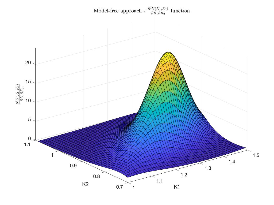
Refer to caption
Refer to caption
Figure 6.5: Implied scaled density surface and contour plot for the three currency pairs for a range of strikes K1K_{1} and K2K_{2}.

References

  • [1] P. Austing. Repricing the cross smile: an analytic joint density. Risk, July:72–75, 2011.
  • [2] P. Austing. Smile Pricing Explained. Palgrave Macmillan, 2014.
  • [3] E. Benhamou, E. Gobet, and M. Miri. Time dependent Heston model. SIAM J. Finan. Math., 1:289–325, 2010.
  • [4] T. Bjork. Arbitrage Theory in Continuous Time. Oxford University Press, 2009.
  • [5] A. Castagna. FX Options and Smile Risk. Wiley, 2010.
  • [6] I. Clark. Foreign Exchange Option Pricing: A Practitioners Guide. Wiley, 2011.
  • [7] Z. Dadachanji. FX Barrier Options: A Comprehensive Guide for Industry Quants. Springer, 2016.
  • [8] A. De Col, A. Gnoatto, and M. Grasselli. Smiles all around: FX joint calibration in a multi-Heston model. J. Banking & Fin., 37(10):3799–3818, 2013.
  • [9] S. De Marco and C. Martini. Moment generating functions and normalized implied volatilities: unification and extension via Fukasawa’s pricing formula. Quant. Fin., 18:609–622, 2018.
  • [10] S. del Baño Rollin. Spot inversion in the Heston model, CRM Prepint 837, 2008.
  • [11] P. Doust. The intrinsic currency valuation framework. Risk, pages 89–95, July 2008.
  • [12] P. Doust. The stochastic intrinsic currency volatility model: a consistent framework for multiple FX rates and their volatilities. Appl. Math. Fin., 19(5):381–445, 2012.
  • [13] P. Doust and J. Chen. Estimating intrinsic currency values. RISK, pages 76–81, 2007.
  • [14] E. Eberlein, A. Papapantoleon, and A. N. Shiryaev. On the duality principle in option pricing: semimartingale setting. Finance Stoch., 12:265–292, 2008.
  • [15] M. Fukasawa. The normalizing transformation of the implied volatility smile. Math. Fin., 22:753–762, 2012.
  • [16] H. Geman, N. El Karoui, and J.-C. Rochet. An exact bond option pricing formula. J. Appl. Prob., 32(2):443–458, 1995.
  • [17] A. Gnoatto and M. Grasselli. An affine multicurrency model with stochastic volatility and stochastic interest rates. SIAM J. Finan. Math., 5(1):493–531, 2014.
  • [18] J.O. Grabbe. The pricing of call and put options on foreign exchange. J. Int. Money Financ., 2:239–253, 1983.
  • [19] L.A. Grzelak and C.W. Oosterlee. On the Heston model with stochastic interest rates. SIAM J. Financial Math., 2:255–286, 2011.
  • [20] P. S. Hagan, D. Kumar, A. S. Lesniewski, and D. E. Woodward. Managing smile risk. The Best of Wilmott, page 249, 2002.
  • [21] S.L. Heston. A closed-form solution for options with stochastic volatility with applications to bond and currency options. The Review of Financial Studies, 6(2):327–343, 1993.
  • [22] F. Jamshidian. An exact bond option pricing formula. J. Finance, 44(1):205–209, 1989.
  • [23] R. Lee. The moment formula for implied volatility at extreme strikes. Math. Fin., 14:469–480, 2004.
  • [24] A. Lipton. Mathematical Methods for Foreign Exchange: a Financial Engineer’s Approach. WSPC, 2001.
  • [25] W. Margrabe. The value of an option to exchange one asset for another. J. Finance, 33:177–186, 1978.
  • [26] D. Reiswich and U. Wystup. FX volatility smile construction. Wilmott, 2012(60):58–69, 2012.
  • [27] F. D. Rouah. The Heston Model and its Extensions in Matlab and C. John Wiley & Sons, 2013.
  • [28] J. Siegel. Risk, interest rates and the forward exchange. Quart. J. Econ., 86(2):303–309, 1972.
  • [29] R. Stulz. Options on the minimum or maximum of two assets: Analysis and applications. J. Fin. Econ., 10:161–185, 1982.
  • [30] U. Wystup. FX Options and Structured Products. Wiley, 2007.