Human Whole-Body Dynamics Estimation for Enhancing Physical Human-Robot Interaction
Claudia Latella
Supervisor: Dott. Francesco Nori
Fondazione Istituto Italiano di Tecnologia
Dynamic Interaction Control Lab
Genova, Italy
Dipartimento di Informatica, Bioingegneria, Robotica e Ingegneria dei Sistemi, Università di Genova
Abstract
In the last two decades the scientific community has shown a great interest in understanding and shaping the interaction mechanisms between humans and robots. The interaction implies communication between two dyadic agents and, if the type of interaction is ‘physical’, the communication is represented by the set of forces exchanged during the interaction. Within this context, the role of quantifying these forces becomes of pivotal importance for understanding the interaction mechanisms. At the current scientific stage, classical robots are built to act for humans, but the scientific demand is going towards the direction of robots that will have to collaborate with humans. This will be possible by providing the robots with sufficient pieces of information of the agent they are interacting with (i.e., kinematic and dynamic model of the human). In a modern age where humans need the help of robots apparently in an opposite trend this thesis attempts to answer the following questions: “Do robots need humans? Should robots know their human partners?”. A tentative answer is provided here in the form of a novel framework for the simultaneous human whole-body motion tracking and dynamics estimation, in a real-time scenario. The framework encompasses a set of body-mounted sensors and a probabilistic algorithm able of estimating physical quantities that in humans are not directly measurable (i.e., torques and internal forces). This thesis is mainly focussed on the paramount role in retrieving the human dynamics estimation but straightforwardly it leaves the door open to the next development step: passing the human dynamics feedback to the robot controllers. This step will enable the robot with the capability to observe and understand the human partner by generating an enhanced (intentional) interaction.
Acknowledgements
First of all, I would like to thank Francesco (Nori) for the opportunity he gave me three years ago: they have been, professionally and personally speaking, very beautiful years. To Francesco (Romans) for helping, supporting and tolerating me and to Daniele for being a great friend of mine before that of a colleague. To Silvio for his constant help and for what he has developed throughout these years: he gave us a solid foundation on which developing our work.
To the new An.Dy group. To Luca (Tagliapietra), he was the last one to arrive but he is already a companion of a thousand misadventures (or ‘disagi’, as we prefer to call them). To Yeshi, our new control man, for his important contribution to the human-in-the-loop stuff! And to Diego, our technician. But above all, to Marta and Maria, our M&M’s: even if they are not currently part of our group, they collaborated in the past to build what the human research line is now . For me, they will be always An.Dy girls!
To all my lab colleagues (of today and of the past): Gabry, Stefano, Aiko, Nuno, Luca (Fiorio), Jorh, Joan, Marie, Francisco, La Strama, Alessia, Boiello e Matte, and to the new comers! To the big purchases with Marianna and Angelica Rosboff.
To Dana for the opportunity she gave me to visit her labs in Waterloo and to meet the Waterloo guys. To those of them that helped me with the setup (Jonathan, Vlad and Kevin) and to those ones that have been subject to the experiments.
To my loved ones for rooting for me: to my parents, my sister Katia and his boyfriend Silvio, my aunt Clelia, my husband’s family (Mariarosa, Pierluigi, Giacomo, Sara and Filippo) for their support and all my friends.
And to Paolo, if I am here today I owe it to him, to that extreme fortitude to which he hanged up in a moment of extreme pain and difficulty. Thanks for giving me this, too!
… And to those (non-scientific) filters that allow me to move forward!
Preliminaries
The following lists represent reference tables for the entire manuscript.
Nomenclature
| Scalar (non-bold small letter) | |
| Vector (bold small letter) | |
| Matrix, tensor (bold capital letter) | |
| Transpose matrix | |
| Cross product for D motion vectors | |
| (Dual) cross product for D force vectors | |
| Matrix determinant | |
| Skew-symmetric matrix | |
| Matrix, tensor (bold capital letter) | |
| Coordinate reference frame (calligraphic letter) | |
| Origin of coordinate frame | |
| Vector expressed in frame | |
| Transformation operator from frame to frame | |
| First-order time derivative | |
| Second-order time derivative | |
| Spatial vector (underlined bold small letter) | |
| Inertia tensor | |
| Jacobian matrix | |
| Motion freedom subspace | |
| Summation operator | |
| Pseudoinverse of a matrix | |
| Inverse matrix | |
| Rank of a matrix | |
| Normal distribution | |
| Expected value | |
| Mean | |
| , | Covariance matrix |
| Maximizing argument | |
| Minimizing argument | |
| Diagonal matrix | |
| Norm | |
| Trace |
Abbreviations and Acronyms
| HRI | Human-Robot Interaction |
| pHRI | Physical Human-Robot Interaction |
| w.r.t. | With respect to |
| D | Two-dimensional |
| DoF | Degree of Freedom |
| ID | Inverse Dynamics |
| IMU | Inertial Measurement Unit |
| D | Three-dimensional |
| RGB | Red-Green-Blue |
| D | Six-dimensional |
| CoM | Centre of Mass |
| RNEA | Recursive Newton-Euler Algorithm |
| URDF | Unified Robot Description Format |
| fb | Fixed base |
| Probability Density Function | |
| MAP | Maximum-A-Posteriori |
| MSE | Mean Square Error |
| MMSE | Minimum Mean Square Error |
| LMMSE | Linear Minimum Mean Square Error |
| GLS | Generalized Least-Squares |
| IK | Inverse Kinematics |
| F/T | Force/Torque |
| RMSE | Root Mean Square Error |
| API | Application Programming Interface |
| YARP | Yet Another Robot Platform |
| EM | Expectation-Maximization |
| EKF | Extended Kalman Filter |
Chapter 1 Introduction
Any sufficiently advanced technology is indistinguishable from magic.
Arthur C. Clarke
1.1 Rationale
Human-Robot Interaction (HRI) is arousing a remarkable interest among the scientific community. The field, emerged in the early years of , addresses the design, the understanding and the evaluation of robotic systems which involve humans and robots interacting through cooperation.
The ever-growing interest of the scientific community in studying coupled human-robot systems is visible in the thriving production of papers related to HRI topics in the last two decades. Figure 1.1 shows the number of papers obtained by searching on the IEEE Explore website the keyword ‘human-robot’ concerning the two main conferences of robotics: IEEE/RSJ International Conference on Intelligent Robots and Systems (IROS) and IEEE International Conference on Robotics and Automation (ICRA). Despite the existence of several fluctuations over the years, the trend has definitely increased straddling the two centuries (see also (Demircan et al. 2015)).

The HRI problem is well-defined as the problem “to understand and shape the interactions between one or more humans and one or more robots. […] evaluating the capabilities of humans and robots, and designing the technologies and training that produce desirable interactions are essential components of HRI. Such work is inherently interdisciplinary in nature, requiring contributions from cognitive science, linguistics, and psychology; from engineering, mathematics, and computer science; and from human factors engineering and design” (Goodrich and Schultz 2007). This definition clearly highlights the multidisciplinarity of the field and justifies the ever-increasing interest of the scientific community in dealing with it.
The word interaction is synonym of communication. The taxonomy of an interaction is highly vast and therefore the concept of communication is different depending on whether it is a remotely-controlled or a proximate interaction. If we consider those applications that require physical HRI (pHRI), this communication is not intended to be verbal (or visual) but it is the result of a set of forces exchanged between the interacting agents.
Nowadays, the demand for physical robotic assistance to humans is a widening practice. Robotic devices are largely widespread in many fields for fulfilling practical, and very different, daily applications such as industrial manipulators for the assembly-lines context, assistive and rehabilitative technology in clinical scenarios. By googling the keywords ‘human-robot physical interaction’, it is easy to find on the web a huge amount of pictures where humans and robots are asked to share a common working space and to cooperate in order to accomplish a required task (Figure 1.2).


The modern and advanced robots are equipped with force and tactile sensors to measure contact forces and actuators to control them with reactive strategies. But physical collaboration also requires anticipatory strategies for predicting the posture (i.e., where the human is located with respect to (w.r.t.) the robot peripersonal space) and the forces applied by the collaborative partner. At the current scientific stage, classical robots are built to act for humans, but in order to adapt their functionality to the current technological demand, the new generation of robots will have to collaborate with humans. The new frontiers in the pHRI field will deal with the development of robotic systems that will be able to react, interact and collaborate with people. This implies that the robots will be endowed with the capability to control physical collaboration through intentional interaction with humans. To achieve an effective collaboration, the robots have to be aware of who the human partner is (in terms of modelling), both in terms of positions (motion) and in terms of dynamics (contacts and exchanged forces, internal forces, joint torques). However the current state of the robot knowledge in observing human whole-body dynamics yields to non-proficient and unadaptive interactions.
To overcome this drawback, it is fundamental to understand what the response of the human body is while a physical interaction is occurring. The importance in retrieving this information is exemplified in Figure 1.3: once the human dynamics is completely known, the human feedback may be provided to the robot controllers. As a straightforward consequence, the robot may accordingly adjust the strategy of the interaction to enhance in this way the common aim of the task. This kind of online awareness in the robot controllers will be the key to bridge the current limitation of robots in observing the human dynamics.
1.2 State of the Art
The aim of this Section is to provide an overview of what is the current state and the direction of the scientific community on the topics covered by this thesis. To this purpose, it was necessary to split it into three main macro-areas concerning the state of the art on the methodologies for estimating the human dynamics, the current state of the sensor technology available on the market and the research status on the pHRI topic.
1.2.1 Human Body Dynamics Estimation
The knowledge of the human body internal forces and joint torques is of pivotal importance in understanding the human dynamics. The procedure for retrieving these variables starting from the measured motion quantities is referred to as the Inverse Dynamics (ID) estimation problem.
Given a human body model composed by interconnected segments, the common mathematical approach iteratively solves the Newton-Euler equations for each model segment. The approach differs depending on the available input data, following two different paths (Winter 1990) (see Appendix A).
- •
A version that solves iteratively the Newtonian physics from the top-most to the bottom-most segment (i.e., top-down approach) by the means of only angular acceleration measurements. However, the joint torques estimation is highly sensitive to uncertainties in acceleration data since they are retrieved by a double differentiation of the positions and, therefore, this method tends to produce noisy and non-reliable estimations (Cappozzo et al. 1975).
- •
A modified version that encompasses additional measurements in the form of ground reaction forces. The method, also called bottom-up, starts at the bottom-most segment where further boundary conditions are provided (typically ground reaction forces from force plates) and proceeds towards the top-most segment. Typically it produces more precise estimations but the introduction of additional data provides more equilibrium conditions to be satisfied: the problem arises at the top-most segment where the physics conditions are not satisfied anymore.
In general, when an additional measurement is introduced into the computation, a further constraint has to be defined at the final segment (both for top-down or bottom-up methods) in order to satisfy the equations of motion. This is due to the fact that the system of equations becomes overdetermined. The solution is retrieved by discarding equations and it is strongly dependent on which equations are discarded, as recognized by (Kuo 1998) that treats the problem of finding the joint torques as a least-squares problem. The idea here is to find a set of joint torques that best agrees with the available data and to exploit the redundancy of the system when some measurements are missing or unreliable. The main drawback is that it is applicable only to a D fixed-base system. In a subsequent study (van den Bogert and Su 2008), a further development of (Kuo 1998) is presented, not restricted to D fixed-base system but particularly tailored for gait analysis. The method solves ID problems where the number of the unknown variables does not exceed the degrees of freedom (DoFs) of the system by employing a weighting covariance matrix derived via Monte Carlo simulation of measurement errors.
The least-squares approach became very popular for solving the human ID estimation since it is a versatile tool for addressing optimization problems solution. Since it is historically well-known that ID accuracy is closely related to the reliability of the accelerations data (Challis and Kerwin 1996), a weighted least-squares optimization approach is adopted in (Cahouët et al. 2002) to retrieve optimum acceleration estimates from all the available imperfect and redundant measurements (positions by markers and forces by force plates). Since the considered cost function does not contain information on the joint torques, the method is not so robust to errors in the joint torque estimation. In (Riemer and Hsiao-Wecksler 2008), a similar methodology is used but combining two important factors: a cost function that minimizes the difference between the measured ground reaction forces and the forces estimated via a top-down approach; an optimization criterion for the measured joint angles.
1.2.2 Sensors Technology
Several commercial solutions for the whole-body motion tracking are available on the market. The standard approach for motion detecting is a marker-based technology for in-lab applications produced by Vicon or MotionAnalisys. A more recent approach is to supplement or even replace marker-based technologies in several applications with wearable markerless technologies suitable for outdoor motion capturing produced by Xsens or Noraxon, where markers are replaced by body-mounted Inertial Measurement Units (IMUs). Another kind of solution is provided by the Microsoft Kinect depth camera system which allows markerless low-cost whole-body motion tracking for indoor applications (Zhang 2012).
In biomechanics, soft wearable and stretchable systems have been proposed for measuring human body motion (Mengüç et al. 2013) (Mengüç et al. 2014), as well as in health activity monitoring (Paradiso and Rossi 2006) (Gallego et al. 2011). Combinations of different technologies have also been used for detecting human motion: in (Wei and Chai 2010), a video-based motion technique has been adopted for capturing realistic human motion from video sequences.
Although these existing technologies provide a high level of accuracy in computing motion quantities, they have several limitations in measuring real-time dynamics quantities (i.e., forces and torques). A key problem lies in the fact that motion capture methods typically employ only kinematic measurement modalities (positions, velocities and accelerations) (Bonnet et al. 2013) and do not include sufficient information on the dynamics of the human movements.
The importance of including and exploiting dynamics information is a crucial point in several research areas such as ergonomics for industrial scenarios, rehabilitation monitoring, for developing prosthetic devices and exoskeleton systems or in pHRI scenarios. For these reasons, the whole-body force tracking is not a new challenge for the scientific community, but the topic has been seldom explored in situ and even more rarely analyzed in real-time modality (this step requires the development of estimation algorithms to be coupled to the sensors).
To overcome the drawbacks related to the in-lab force tracking acquisitions (usually attained through the combination of a motion capture system with commercial force plates), several solutions of pressure sensing insoles are available on the market, such as Moticon or Tekscan used in (Zhang et al. 2014). However, prototypes of sensing shoes have been proposed in the recent scientific scenario: a prototype of wearable shoes developed by Xsens (Schepers et al. 2007) and a sensory system for the foot pressure evaluation tailored for exoskeletons applications (Mateos et al. 2016).
1.2.3 Physical Human-Robot Interaction
Most of the pHRI studies take inspiration from the intrinsic behaviour of the human nature: the mutual adaptive nature that automatically occurs when two humans are cooperating together to accomplish a common task. To this purpose, the importance of understanding the human dynamics goes without saying and it is a crucial aspect of current scientific research.
Based on the pioneering study on the minimum-jerk model in human manipulation tasks (Flash and Hogan 1985), a method based on the minimization of the jerk is used as a suitable approximation for estimating the human partner motions in (Maeda et al. 2001) during a human-robot cooperative manipulation. Here the authors’ attempt is to incorporate human characteristics into the control strategy of the robot. The weakness in this type of approach lies in the pre-determination of the task and in the role that the robot has to play in the task execution. Furthermore, the minimum-jerk model reliability decreases considerably if the human partner decides to apply non-scheduled trajectory changes during the task (Miossec and Kheddar 2009).
Another suitable route for pHRI is the imitation learning approach, justified by a wide variety of computational algorithms that have been developed by the scientific community in the past decades (see an exhaustive overview in (Schaal et al. 2003)). This approach yields to the teacher-student (or more pragmatic master-slave) interaction concept and consists in the following steps:
- •
Collection of human motions: movements of a human agent (i.e., the teacher in the imitation process) are retrieved with motion capture techniques and clustered in motion databases. Some publicly available examples are (Guerra-Filho and Biswas 2011) (Kuehne et al. 2011) (Wojtusch and von Stryk 2015) (C. Mandery and Asfour 2015).
- •
Classification for model abstraction: human motions are classified via motion segmentation in order to abstract motion models. The model abstraction is feasible by postulating that the human movements can be decomposed into a set of primitive actions, termed motion primitives.
- •
Models retargeting: human motion models are mapped into a robot platforms, i.e., the student in the imitation process. The retargeting implies the development of robot control algorithms capable of learning motion models from these primitives (Amor et al. 2014) (Terlemez et al. 2014), (Mandery et al. 2016) in order to emulate human-like movements.
Since the primitives have to be perceived and interpreted by a robot, a common ‘language’ has to be mandatorily adopted. The abstraction implies, therefore, to define the primitives in terms of positions, velocities and accelerations. In a recent work (Borràs et al. 2017), the collection of human motions is performed when the human is interacting with the external environment and exploiting multi-contact support to enhance his stability. Here, the classical characterization of a primitive (through the kinematic above-mentioned variables) is coupled with the important information on how the human is maintaining his stability.
In general, although in the imitation approach the task pre-determination does not represent a drawback anymore, a relevant problem (termed correspondence problem) concernes the comparability of the models (teacher vs. student). Human motion primitives are exploitable only if their knowledge could be properly mapped into a compatible robot kinematic/dynamic model. This inevitably narrows down the potential student-role candidate to anthropomorphic robots and it requires an accurate analysis on the imitation mechanism assumptions.
1.3 Contribution
The thesis contribution lies in the development of a novel wearable technology for the simultaneous force and motion human tracking. The attempt of this work is to bridge the current state-of-the-art gap on human dynamics analysis thanks to
- •
a combination of different sensors (body-mounted IMUs, force sensing)
- •
a whole-body force estimation algorithm, originally developed for the humanoid iCub robot (Nori et al. 2015) and tailored here for the human body.
The novelty of the approach consists in framing the dynamics computation in a probabilistic Gaussian framework when redundant measurements occur. In this way, sensors play an active role in the computation since the classical boundary conditions in the recursive Newton-Euler algorithm are replaced with the sensors readings. The estimation algorithm solves a sort of weighted least-squares problem where the weights are given by the dynamic model and the sensors.
1.3.1 Publications
Here following the list of the related publications (at the time of writing) produced during my Ph.D. course period:
- •
Romano, F.; Nava, G.; Azad, M.; Camernik, J.; Dafarra, S.; Dermy, O.; Latella, C.; Lazzaroni, M; Lober, R.; Lorenzini, M.; Pucci, D.; Sigaud, O.; Traversaro, S.; Babic, J.; Ivaldi, S.; Mistry, M.; Padois, V.; Nori, F. “The CoDyCo Project achievements and beyond: Towards Human Aware Whole-body Controllers for Physical Human Robot Interaction”, Special issue on Human Cooperative Wearable Robotic Systems in IEEE Robotics and Automation Letters, :-, November 2017. (RA-L), , PP, . doi: 10.1109/LRA.2017.2768126, http://ieeexplore.ieee.org/document/8093992.
- •
Latella, C.; Kuppuswamy, N.; Romano, F.; Traversaro, S.; Nori, F. “Whole-Body Human Inverse Dynamics with Distributed Micro-Accelerometers, Gyros and Force Sensing”, Sensors , , . doi: 10.3390/s16050727, http://www.mdpi.com/1424-8220/16/5/727.
- •
Latella, C.; Kuppuswamy, N.; Nori,F. “WearDY: Wearable dynamics. A prototype for human whole-body force and motion estimation”, AIP Conference Proceedings , (). doi: http://dx.doi.org/10.1063/1.4954494.
1.4 Technological Outcome
The framework proposed in this thesis is the core of the Horizon- European project named An.Dy - Advancing Anticipatory Behaviors in Dyadic Human-Robot Collaboration (H-ICT--, No.) (An.Dy 2017). The project aims at advancing the current state of the art in the pHRI field by providing a novel wearable technology that measures human whole-body dynamics and, in turns, endows robots with the ability to be more aware of the human partner they are interacting with. An.Dy will enhance the intentional cooperation between humans and robots. The results achieved in this thesis represent the entry point and the basis on which An.Dy will lay its foundations in the next years.
1.5 Thesis Outline
Hereafter, a brief summary of the topics of the thesis is provided. Each chapter briefly introduces the topic and starts (if needed) with the notation useful for guiding the reader into its comprehension.
Chapter 2 introduces a complete overview of the kinematics and the dynamics of a rigid body and, then, of a system of rigid bodies.
Given the notions from the previous chapter, Chapter 3 describes the human whole-body modelling as a system of articulated rigid bodies.
In Chapter 4, the human dynamics estimation problem is presented and it is provided a solution in a probabilistic domain.
Chapter 5 describes the Matlab software implementation for the offline validation of the framework. It shows the sensing technologies used for the algorithm and introduces also a new wearable prototype developed at Istituto Italiano di Tecnologia for measuring ground reaction forces.
The main contribution of Chapter 6 is the design of a YARP tool for the real-time monitoring of the human dynamics.
Chapter 7 discusses the possibility to extend the human dynamics estimation fremework to a new framework where a physical interaction with the iCub robot is encompassed.
Chapter 8 concludes the thesis with a general overview on the obtained preliminary results and analyzes possible improvements as forthcoming works.
Chapter 2 Rigid Multi-Body System
Nothing happens until something moves.
Albert Einstein
In this Chapter a complete overview of the kinematics and the dynamics of a rigid multi-body system is introduced. For achieving this objective, a detailed description of the ‘sub-units’ that describe a multi-body system is mandatorily needed. The sub-units are the bodies and the joints which a system is made of. The reader will be provided with some tools that describe the kinematics and the dynamics of a rigid body and, only then, with the multi-body system notions.
2.1 Notation
Hereafter some important math preliminaries adopted through the thesis.
- •
Let be the set of real numbers. is a -dimensional column vector of real numbers. Let denote a scalar quantity.
- •
A matrix of dimensions .
- •
Let be the identity matrix of dimension .
- •
Let be the zero matrix and .
- •
Given two generic vectors , , their inner product is denoted with . The cross product is denoted as , where
(2.1) - •
Given a vector and a reference frame , the notation denotes the vector expressed in .
- •
Let be the set of orthogonal matrices with determinant equal to one, such that
(2.2) - •
Let be the set of the skew-symmetric matrices , such that
(2.3) - •
Let the set be defined as
(2.4)
2.2 The Non-Deformability Assumption
In the physics formalism, a rigid body is represented as a body which does not deform under the application of an external force. This means that the distance between two generic points in the body does not vary when a force is exerted on it, i.e., the body is non-deformable. In real life, this utopian condition does not exist. There are situations in which the body deforms depending , for example, on the magnitude or the point of application of a force. However, under the hypothesis that the deformation is small, i.e., negligible, the rigid body assumption allows to describe the dynamics of every physical object.
2.3 Rigid Body Kinematics
The kinematics of a rigid body concerns the mechanism of its motion without considering the forces and torques that caused it. Among the robotics community, the most influential description of the rigid body kinematics (Siciliano and Khatib 2007) (Siciliano et al. 2008) is through its position and its orientation w.r.t. a known coordinate reference frame. The body velocity and acceleration depend on this representation.
2.3.1 Pose Representation
The rigid body kinematics can be described by the pose representation, i.e., the position and orientation w.r.t. a reference frame. Let the frame (i.e., ‘inertial’) be a reference frame with the origin in a 3D point . Let (i.e., ‘body’) be another frame with the origin in the 3D point attached to the rigid body. Consider now that moves w.r.t. . Every type of motion of the body (translation, rotation or a combination of the two) will produce a variation in its pose. This means that the pose representation becomes a powerful tool for describing the entire kinematics of the rigid body.
The coordinates of the point w.r.t. are clustered in the position vector whose origins in and points to , such that
| (2.5) |
The Rotation Matrix
The orientation of w.r.t. is described by a rotation matrix , regardless of the positions of the origins and . Additionally, the rotation matrix can be seen as a tool for operating coordinates transformation between two frames: given a point (in Figure 2.1) and its coordinates vector expressed in , the rotation matrix transforms its coordinates from the frame to the frame , such that
| (2.6) |
The Homogeneous Transformation
The formalism that best summarizes the pose of a rigid body is the homogeneous transformation matrix . Let , be two vectors , i.e., , , such that
| (2.7) |
being
| (2.8) |
The Equation (2.8) is a compact way to represent the position along with the rotational component of the motion. If (i.e., null position vector ), (2.7) falls into the pure rotational case (2.6). If the frame is not rotated w.r.t. (i.e., the rotation matrix ) thus (2.7) becomes .
It is worth noting that, throughout the thesis, the reference frames are shown using a RGB (Red-Green-Blue) convention for -- axes, respectively.
2.3.2 The Derivative of a Rotation Matrix
In this framework, the derivative of the rotation matrix raises with particular emphasis since it allows to describe the velocity and the acceleration of a rigid body. Even if not explicitly defined in the text, consider a time-varying matrix. It is shown (and the reader is addressed to (Siciliano et al. 2008), Section 3.1.1, for a detailed description) that there is a straightforward relation between and the skew-symmetric operator , such that
| (2.9) |
Velocity
Given an inertial frame , a body reference frame and a point P of the body (Figure 2.2), for (2.7) we can define the following equation
| (2.10) |
The velocity of P w.r.t. can be obtained by using the first-order time derivative of (2.10), such that
| (2.11) |
It is worth noting that is not a time-varying quantity as a direct consequence of the non-deformability assumption of the body (see Section 2.2). Equation (2.9) yields to , thus in (2.11)
| (2.12) |
If is the angular velocity of the frame w.r.t. , thus the above equation can be written as
| (2.13) |
This implies that is actually the skew-symmetric matrix for the angular acceleration, such that
| (2.14) |
Acceleration
Similarly, the acceleration of P w.r.t. can be obtained by using the second-order time derivative of (2.10), such that
| (2.15) | |||||
2.3.3 6D Motion Vectors
A D motion vector represents a spatial vector of a quantity that describes the motion of a body (e.g., the velocity and the acceleration). Given a generic spatial vector , the three first entries are the coordinates of its linear part , and the last three entries represent the angular part of the same quantity, such that
| (2.16) |
Within this new formalism, the velocity (i.e., the spatial velocity) of the rigid body expressed w.r.t. can be written as
| (2.17) |
Similarly, the spatial notation for the acceleration (i.e., the spatial acceleration) of the rigid body expressed w.r.t. is
| (2.18) |
Adjoint Transformation for Motion Vectors
When dealing with spatial vectors, the change of frame can not be performed by using an homogeneous transformation but it has to be introduced a new transformation matrix, i.e., the adjoint matrix define as follows.
Let and be two generic frames and the position vector of the origin of w.r.t. , thus the adjoint transformation is
| (2.19) |
such that
| (2.20) |
The Cross Product for Motion Vectors
Within the framework of the motion vectors, the cross product operator as previously defined is not useful anymore. In (2.1) it is defined in while now we are operating in the new formalism. Thus, it has to be properly modified for matching the spatial context.
Consider a rigid body with a body frame that is moving with a spatial velocity , as defined in (2.17). If the generic vector is a motion vector (e.g., the spatial acceleration of the body), thus their cross product is
| (2.21) |
In particular, the cross product operator is such that
| (2.22) |
where it is easy to identify in the term the skew-symmetric matrix defined as in Equation (2.14).
2.4 Rigid Body Dynamics
In classical mechanics, the dynamics is that branch concerned with the study of the forces and torques and their effect on the motion of a body. It is worth remarking that although sometimes it is referred to this branch as the kinetics of the rigid body (Winter 1990) (Robertson et al. 2014), we prefer here to address to the dynamics (as in (Siciliano and Khatib 2007) (Featherstone 2007)). Clearly the reader has to know that the two definitions are completely equivalent.
2.4.1 6D Force Vectors
Similarly to the motion vector case, also in the context of dynamics it is possible to define a specific class of D vectors related to the force. As previously, a force vector contains a pair of D vectors: the first vector represents the resultant of the forces acting on the body, the last one is referred to the moments produced by the resultant w.r.t. a given point. This yields to the following notation:
| (2.23) |
Adjoint Transformation for Force Vectors
The adjoint transformation for a D force vector is
| (2.24) |
such that
| (2.25) |
being , and , two generic frames and the position vector of the origin of w.r.t. , respectively.
The (Dual) Cross Product for Force Vectors
Similarly to the cross product for the motion vectors, we have a cross product for the force vectors that is the dual version of (2.22). Within the same framework explained for the motion case , we have
| (2.26) |
such that
| (2.27) |
2.4.2 The Newton-Euler Equations of Motion
The equations of motion describe the mathematical model for the dynamics of the rigid body. Within the spatial formalism, it is possible to write the equations of motion as
| (2.28) |
where the force of a rigid body that is moving with velocity and acceleration is equal to the rate of change of its momentum . In Equation (2.28),
- •
in the net force acting on the rigid body;
- •
is the spatial inertia tensor , such that
(2.29) where is the inertia tensor w.r.t. the link center of mass (CoM), m is the body mass, is the position vector from the CoM of the body to the origin of the body frame ;
- •
the term is the operator that maps to its derivative .
2.5 Rigid Multi-Body System
A rigid multi-body system is a system composed of two or more interconnected rigid bodies. The resulting motion of a system is obtained by composing elementary motions of each body w.r.t. the coupled one. The mobility of the system is ensured by the presence of the joints: each joint interconnects two bodies and constraints their motion. The type of motion is strongly related to the type of joint but the description of the different types of joints is out of the scope of the thesis. Thus, they will be described in detailed only when required for the thesis understanding.
2.5.1 Modelling
Within a classical widespread formalism in robotics (Featherstone 2007) (Siciliano et al. 2008), an articulated rigid multi-body system is represented as a kinematic tree composed of rigid bodies. The topology of the system (i.e., the interconnectivity property) is such that it is often referred to it as a tree system. Under the tree schematization formalism, the bodies are the nodes and the connection between them are the joints. Each rigid body in the system is associated to a unique node in the tree.
Let be the number of moving rigid bodies of the system whose topological numbering is defined from to ( refers to the fixed base). Let be the index for a generic body in the tree such that . Node numbers can be always selected in a topological order so that the -th node has a higher number than its unique parent and a smaller number than all the nodes in the set of its children .
The -th body and its parent are coupled with joint according to the Denavit-Hartenberg convention for joint numbering (Denavit and Hartenberg 1955). The motion freedom subspace of the -th joint is modelled with , being the DoFs number of the joint . Within this notation, = + + represents the internal DoFs of the system. Figure 2.3 shows a connectivity system representation for the kinematic tree.
2.5.2 Lagrangian Representation
A common representation of the dynamics of the system is derived from the Lagrangian formalism. Given a rigid multi-body system with internal DoFs, by rearranging the Lagrange formulation (the reader could refer to several robotics textbooks like (Siciliano et al. 2008), Chapter 7), it is possible to define its floating-base dynamics representation11 1 Representation in which none of the links have an a priori constant pose w.r.t. the inertial frame. as follows:
| (2.30) |
where is the mass matrix, is the Coriolis effects matrix, is the gravity bias term.
In general, a floating-base system is defined by its configuration and its velocity , where is the inertial frame and the base frame. is the homogeneous transformation from to and is the base velocity w.r.t. . The configuration and the velocity of the internal DoFs are denoted with and , respectively. The system can interact with the external environment and this results in the presence of , where is the number of the forces exchanged during the interaction. The Jacobian associated with the forces is denoted by and the vector represents the joint torques of the system.
Throughout the thesis the human experiments will be performed with the feet fixed to the ground. We limit to consider therefore the human system to be fixed base, i.e., and known a priori and . This choice straightforwardly implies and allows to reduce remarkably the framework complexity. These assumptions yield to a simplified version of (2.30), such that
| (2.31) |
2.5.3 Newton-Euler Representation
The Newton-Euler formulation is an equivalent way to the Lagrangian formalism for representing the dynamics of a multi-body system. It is based on the balance of the forces acting on each body composing the structure of the system and leads to a set of recursive equations for propagating the kinematics and dynamics quantities throughout the system.
Consider a system of rigid bodies connected by joints. The topology and the body numbering are defined as in Section 2.5.1. Let be the fixed base. If , the velocity of the -th link and the velocity through the -th joint are defined recursively as follows:
| (2.32) | |||||
| (2.33) |
Given Equations (2.32) and (2.33), the recursive Newton-Euler algorithm (RNEA) consists of the following steps, expressed in body coordinates22 2 Except for the external forces that are expressed in the body absolute coordinates.:
| (2.34) | |||||
| (2.35) | |||||
| (2.36) | |||||
| (2.37) |
Equations (2.32), (2.33) and (2.34) are propagated throughout the kinematic tree with the initial boundary conditions and , which corresponds to the gravitational spatial acceleration vector expressed in the body frame , such that . Equation (2.35) is exactly the equation of motion for the -th body described in (2.28) and represents here the net force acting on the body. Equation (2.36) is the result of a balance of incoming forces (i.e., the internal force transmitted through the -th joint, the external force ) and outgoing forces (namely, the set of internal forces exchanged with the children bodies) w.r.t. the -th link.
Chapter 3 Human Whole-Body Modelling
All models are wrong, but some are useful.
George E. P. Box
In this Chapter a detailed description of the human whole-body modelling is introduced. This is an important step for retrieving the estimation of the human dynamics. The starting point for our analysis is recalled in (Latella et al. 2016) where a simple 2-DoF model was employed for the whole-body modelling. The rough approximation introduced by that model goes without saying and it was useful the ‘upgrade’ to a more complex model able to describe a set of more complex movements.
3.1 Human Whole-Body Modelling
By inheriting the robotics-like formalism described in the Section 2.5.1, we propose a human body model as an articulated multi-body system represented by a kinematic tree with = moving links11 1 Throughout the thesis, it is often referred to a body as a link. The two entities are completely equivalent. ( is the fixed base, e.g., the left foot22 2 At the current stage, the algorithm used for the human dynamics computation requires a fixed-base model. This motivated our choice to consider the left foot as the fixed base (the human subject performed the experimental tasks with the feet fixed on the ground).) and = internal DoFs. The rationale behind the choice of this link number is that we have been guided by the model developed for the Xsens MVN motion capture system (Roetenberg et al. 2009) (Figure 3.1). Since the sensor setup included the Xsens motion capture system, we considered that having two comparable models could be an appropriate choice. This choice is also justified by the fact that the Xsens sensors readings had to be associated to our model.

Several strong assumptions have been considered in designing our model:
- )
to represent the human model as a set of rigid links of simple geometric shape (parallelepipeds, cylinders and spheres);
- )
to consider density isotropy for each link.
In the following sections, it is provided to the reader a detailed description for each of the above-mentioned assumption by motivating through literature our choice.
3.1.1 Inertial Properties Modelling
Inertial properties of link segments, such as mass, centre of mass or moments of inertia, are important parameters in predicting realistic movement patterns. However, these quantities are not directly measurable. More than a century of literature on this topic proves that the importance in retrieving this information has a pivotal role in studying human dynamics. In (Erdmann 1999) the author claims that usually in geometric and inertial investigations, three approches are adopted, by involving living subjects, cadavers and models.
The first investigation (with living subjects) consists in the measurements of the body height and body mass. This type of technique produced over the years well documented anthropometric tables, adopted in the most of inertial studies (Drillis et al. 1964) (Winter 1990) (Herman 2007). These tables correlate the total body mass/height with the mass/height of each link. The second investigation concerns dissections made on cadavers while the model technique is more common in simulation research towards prevention (e.g., car-crash tests).
The author of a more recent study (Robertson 2013) classifies into two macro-categories the methodologies for estimating body inertial parameters: regression equations models and geometric approximation models. The former technique is based on equations derived from cadaveric measurements, computed radiographs, or magnetic resonance imaging of a finite set of specimens. The author reveals the weakness of this approach since it extrapolates data from an average and has little accuracy for modelling a subject that falls outside the proportions of the initial dataset. The other approach consists of a collection of in situ measurements to be mapped into a geometric model to derive mass and properties from certain shape and density assumptions. Here too, the accuracy of the method depends on the complexity of the model and limited to the numbers of measurements. To this purpose, the Hatze model (Hatze 1980) consists of a -segment geometrical model of the body but requires anthropometric measurements, which would imply a relatively substantial amount of time from each subject.
Even if the uniform/non-uniform density assumption is an important part of this analysis (there is an outstanding debate among the scientific community), the complexity and data collection time are the most likely reasons for the lack of the use of Hatze-like model in biomechanical research.
Our approach does not support neither the regression methodology nor the geometrical one. With we opt for a model of simple shapes and offers the possibility of using some analytic formulas to compute the inertial proprieties of all the segments in the model. Under the assumption of density isotropy (Hanavan 1964), the inertia tensor has been computed such that
| (3.1) |
where , and are the principal moments of inertia. Table 3.1 lists analytical formulas for the principal moments of inertia computation.
| Inertia | Parallelepiped | Cylinder | Sphere |
|---|---|---|---|
3.1.2 Link Modelling
The labelling of the human model links is inherited by Xsens biomechanical model. For each link, geometry, dimensions, inertial parameters, origin and orientation have to be mandatorily specified. For the geometry, the links are modelled as parallelepiped boxes, cylinders and spheres. In order to make the model scalable with the subject proportions, the dimension of each shape is obtained via the Xsens IMUs readings33 3 Xsens motion capture system provides as inputs bony landmark points distributed all over the model. We exploit the information of their position in the model for delimiting the predominant dimension of the link geometrical shape.. Inertial parameters are computed by exploiting the anthropometric table (Winter 1990) (Herman 2007): for retrieving the mass of each link the weight of the subject (and thus ) is firstly measured and then the mass of each link is obtained by applying tabulated data. Inertia moments are computed as described in Table 3.1. The origin and orientation of the frame associated to each link are defined in the following way:
| L5 | origin: midpoint on top-face of the Pelvis parallelepiped |
| orientation: pointing forward, pointing upward (line jL5S1-jL4L3) | |
| L3 | origin: midpoint on top-face of the L5 parallelepiped |
| orientation: pointing forward, pointing upward (line jL4L3-jL1T12) | |
| T12 | origin: midpoint on top-face of the L3 parallelepiped |
| orientation: pointing forward, pointing upward (line jL1T12-jT9T8) | |
| T8 | origin: midpoint on top-face of the T12 parallelepiped |
| orientation: pointing forward, pointing upward (line jT9T8-jT1C7) | |
| Neck | origin: midpoint on top-face of the T8 parallelepiped |
| orientation: pointing forward, pointing upward (line jT1C7-jC1Head) | |
| Head | origin: midpoint on top-circle of the Neck cylinder |
| orientation: pointing forward, pointing upward (aligned with jT1C7 axis) | |
| RightUpperLeg | origin: midpoint on top-circle of the RightUpperLeg cylinder |
| orientation: pointing forward, pointing upward (line jRightKnee-jRightHip) | |
| RightLowerLeg | origin: midpoint on top-circle of the RightLowerLeg cylinder |
| orientation: pointing forward, pointing upward (line jRightAnkle-jRightKnee) | |
| RightFoot | origin: point on top-face of the RightFoot parallelepiped |
| orientation: pointing forward, pointing upward (aligned with jRightKnee axis) | |
| RightToe | origin: midpoint on frontal-plane-face (attached to RightFoot) of the RightToe parallelepiped |
| orientation: pointing forward, pointing upward (aligned with jRightKnee axis) | |
| LeftUpperLeg | origin: midpoint on top-cirle of the LeftUpperLeg cylinder |
| orientation: pointing forward, pointing upward (line jLeftKnee-jLeftHip) | |
| LeftLowerLeg | origin: midpoint on top-cirle of the LeftLowerLeg cylinder |
| orientation: pointing forward, pointing upward (line jLeftAnkle-jLeftKnee) | |
| LeftFoot | origin: point on top-face of the LeftFoot parallelepiped |
| orientation: pointing forward, pointing upward (aligned with jLeftKnee axis) | |
| LeftToe | origin: midpoint on frontal-plane-face (attached to LeftFoot) of the LeftToe parallelepiped |
| orientation: pointing forward, pointing upward (aligned with jLeftKnee axis) | |
| RightShoulder∗ | origin: midpoint on sagittal-plane-circle (attached to T8) of the RightShoulder cylinder |
| orientation: pointing forward, pointing right (line jRightC7Shoulder-jRightShoulder) | |
| RightUpperArm∗ | origin: midpoint on sagittal-plane-circle (attached to RightShoulder) of the RightUpperArm cylinder |
| orientation: pointing forward, pointing right (line jRightShoulder-jRightElbow) | |
| RightForeArm∗ | origin: midpoint on sagittal-plane-circle (attached to RightUpperArm) of the RightForeArm cylinder |
| orientation: pointing forward, pointing right (line jRightElbow-jRightWrist) | |
| RightHand∗ | origin: midpoint on sagittal-plane-face (attached to RightForeArm) of the RightHand parallelepiped |
| orientation: pointing forward, pointing right (aligned with jRightElbow axis) | |
| LeftShoulder∗ | origin: midpoint on sagittal-plane-circle (attached to T8) of the LeftShoulder cylinder |
| orientation: pointing forward, pointing right (line jLeftC7Shoulder-jLeftShoulder) | |
| LeftUpperArm∗ | origin: midpoint on sagittal-plane-circle (attached to LeftShoulder) of the LeftUpperArm cylinder |
| orientation: pointing forward, pointing right (line jLeftShoulder-jLeftElbow) | |
| LeftForeArm∗ | origin: midpoint on sagittal-plane-circle (attached to LeftUpperArm) of the LeftForeArm cylinder |
| orientation: pointing forward, pointing right (line jLeftElbow-jLeftWrist) | |
| LeftHand∗ | origin: midpoint on sagittal-plane-face (attached to LeftForeArm) of the LeftHand parallelepiped |
| orientation: pointing forward, pointing right (aligned with jLeftElbow axis) |
3.1.3 Joint Modelling
The links are coupled by joints, whose labels are inherited by Xsens joint labelling. Each joint requires information about the motion type (i.e., the joint DoFs), the origin of the frame associated to it and the links connected through it. For the motion type, the joints of the model are represented with , or DoFs, depending on the anatomy of the relative biological joint. A biological joint is defined as the point where two or more bones articulate. Its functional classification describes the degree of movement allowed between the bones into three anatomical planes: transversal, frontal and sagittal. Thus, the joint motion space is classified as uniaxial (for a movement in one plane), biaxial (for a movement in two planes) or multi-axial joints (for a movement involving three anatomical planes). By classifying the joint motion type, a number of internal DoFs is defined for our modelling. The origin of the frame associated to each joint coincides with the origin of the frames associated to the link. Table 3.4 synthetizes the properties for the joint modelling.
| Label | Shape | Mass of |
|---|---|---|
| Pelvis | parallelepiped | |
| L5 | parallelepiped | |
| L3 | parallelepiped | |
| T12 | parallelepiped | |
| T8 | parallelepiped | |
| Neck | cylinder | |
| Head | sphere | |
| RightShoulder | cylinder | |
| RightUpperArm | cylinder | |
| RightForeArm | cylinder | |
| RightHand | parallelepiped | |
| LeftShoulder | cylinder | |
| LeftUpperArm | cylinder | |
| LeftForeArm | cylinder | |
| LeftHand | parallelepiped | |
| RightUpperLeg | cylinder | |
| RightLowerLeg | cylinder | |
| RightFoot | parallelepiped | |
| RightToe | parallelepiped | |
| LeftUpperLeg | cylinder | |
| LeftLowerLeg | cylinder | |
| LeftFoot | parallelepiped | |
| LeftToe | parallelepiped |
| Label | DoF | Connected links | ||
|---|---|---|---|---|
| jL5S1 | Pelvis | L5 | ||
| jL4L3 | L5 | L3 | ||
| jL1T12 | L3 | T12 | ||
| jT9T8 | T12 | T8 | ||
| jT1C7 | T8 | Neck | ||
| jC1Head | Neck | Head | ||
| jRightHip | Pelvis | RightUpperLeg | ||
| jRightKnee | RightUpperLeg | RightLowerLeg | ||
| jRightAnkle | RightLowerLeg | RightFoot | ||
| jRightBallFoot | RightFoot | RightToe | ||
| jLeftHip | Pelvis | LeftUpperLeg | ||
| jLeftKnee | LeftUpperLeg | LeftLowerLeg | ||
| jLeftAnkle | LeftLowerLeg | LeftFoot | ||
| jLeftBallFoot | LeftFoot | LeftToe | ||
| jRightC7Shoulder | T8 | RightShoulder | ||
| jRightShoulder | RightShoulder | RightUpperArm | ||
| jRightElbow | RightUpperArm | RightForeArm | ||
| jRightWrist | RightForeArm | RightHand | ||
| jLeftC7Shoulder | T8 | LeftShoulder | ||
| jLeftShoulder | LeftShoulder | LeftUpperArm | ||
| jLeftElbow | LeftUpperArm | LeftForeArm | ||
| jLeftWrist | LeftForeArm | LeftHand | ||
3.2 The Human URDF Model
The Unified Robot Description Format (URDF) representation is very common among the robotics community but not widespread among that part of community that deals with human modelling. The reason is quite clear: this format is particularly tailored for describing robots (e.g., the typical specification assumes rigid links) and it does not take into account the presence of muscles in the model (no flexible or shape-variable links are supported). However, two main reasons led us to this choice:
- )
the possibility offered by this format of creating a valid representation for complex tree structures,
- )
the possibility of handling both the models for the human and for the robot with the same formalism.
See Appendix B for a detailed description on how to build the human URDF model.
3.2.1 Sensor Pose Estimation
In order to perform the estimation of the human dynamics, the information about the Xsens IMUs has to be embedded in the URDF model. However, the pose of the sensor w.r.t. the attached link is not provided by Xsens as an output of the system. Therefore, in this Section a procedure for estimating the sensor position by exploiting IMUs linear acceleration and angular velocity is proposed. The procedure is very similar to (Rotella et al. 2016) where it is used for a humanoid robot.
Estimation Procedure
Let be an inertial frame and consider a generic rigid body. We define the body reference frame identifying its pose w.r.t. (Figure 3.2). Consider also a sensor rigidly attached to the rigid body and its reference frame . Let be the gravity acceleration vector expressed in . The estimation problem can be summarized as follows.
The relative orientation between the sensor and the link can be easily obtained by the following equation:
| (3.2) |
To estimate the relative position, consider the measurement equation:
| (3.3) |
where , from (2.9).
To estimate we have to solve Equation (3.2.1). Given that measurements may be affected by errors, it is impractical to solve it with only one measurement. To estimate we thus collect multiple measurements and solve the resulting overdetermined system in the least-squares sense. We first rewrite (3.2.1) in the following form:
| (3.4) |
By denoting with and the matrices and associated with the -th measurement, after collecting measurements we obtain the following linear system:
| (3.5) |
thus
| (3.6) | |||||
| (3.7) |
where denotes the Moore-Penrose pseudoinverse of . Equations (3.7) and (3.2) identify the relative pose of w.r.t. . In the Algorithm 1 the pseudocode for the procedure of sensor position estimation is shown.
A URDF model for the -DoF human template is shown in Figure 3.3. The figure shows the IMUs distributed on the body.

Chapter 4 The Human Dynamics Estimation Problem: a Probabilistic Solution
No great discovery was ever made without a bold guess.
Isaac Newton
In this Chapter, the estimation problem for the human dynamics is investigated. As recalled in Section 1.2.1, the procedure for computing the joint torques given the joint accelerations and the external forces acting on a kinematic tree model is the well-known identified problem of the inverse dynamics. In (Featherstone 2007), the problem is formulated as follows:
| (4.1) |
A classical and computationally efficient solution for the ID problem is the RNEA (presented in Section 2.5.3) which also computes the internal forces and the link accelerations .
We perform here a different choice which encompasses the computation of other human variables (in a new vector ) in a probabilistic domain and includes the sensors measurements (defined in a new vector ). The problem in (4.1) could be therefore written in the form
| (4.2) |
where
- •
the torques of (4.1) are embedded in a new vector ,
- •
the external forces used as input in (4.1) are embedded in a new vector of measurements .
A detailed explanation for the new quantities will follow in Sections 4.1 and 4.2, respectively.
Clearly, there is an unquestionably strong parallelism with the problem (4.1) and over this Chapter it is explained how the classical robotics formalism has been adapted to fit the needs of the human dynamics framework. The Chapter provides the reader with a detailed description of the methodology used for solving the estimation problem whose novelty lies in considering simultaneously the fusion of different sensors information.
4.1 The System Constraints Formulation
Given a suitable model for the human, as in Chapter 3, it is convenient to define a new vector quantity containing variables for describing both the kinematics and the dynamics of the model, with number of bodies and internal DoFs number. If , the vector is such that
| (4.3) |
where
| (4.4) |
It is worth remarking that is a hybrid vector that, by construction, contains quantity related to the -th link (i.e., the acceleration , the net force and the external force ) and the -th joint (i.e., the force exchanged through the joint , the joint torque and the joint acceleration ).
If the Newton-Euler formalism is properly rearranged in a matrix form, thus Equations (2.34)-(2.37) can be considered as a set of linear constraint equations that has to satisfy. Given (4.3) and (4.4), Equations (2.34)-(2.37) can be compactly written in the following matrix equation representing the constraints of the system:
| (4.5) |
where is a block matrix and is a vector , as follows11 1 Note on the notation: it is referred here to . Within this notation is a matrix with rows and columns, i.e., number of rows of (4.3), namely . This form will be recurring throughout the thesis.:
More in detail:
| (4.6) |
| (4.7) |
| (4.8) |
| (4.9) |
| (4.10) |
4.1.1 Considerations on the Representation
Equation (4.5) is an equivalent representation of (2.31). The Lagrangian formulation can be obtained from Equation (4.5) as hereafter described. First, the vector and the columns of should be rearranged so that they respect the following order: , , , , and . The resulting and are:
| (4.11) |
In the human dynamics estimation problem, the choice for preferring (4.5) formulation to (2.31) is two-fold. On the one hand, Equation (4.5) can be used to represent uncertainties that capture relevant modeling approximations. In particular, approximations result from the fact that human bones coupling is neither rigid nor purely rotational and these can be captured with additive noise on Equations (2.34)-(2.37). On the other hand, there are numerical advantages associated to Equation (4.5). In the case of inverse and forward dynamics, the numerical advantages are exactly those obtained by the RNEA presented in (Featherstone 2007) and whose relations to Equation (4.5) is discussed in (Nori et al. 2015).
4.2 The Measurements Equation
Let be the vector containing all the available sensors readings. The explicit equation for the measurements is such that
| (4.14) |
The structure of the matrix depends on how many sensors are considered in the analysis and it is independent from the number of link in the model (more sensors could be associated to the same link, e.g., a combination of an IMU + a force sensor). If number of sensors, thus is a block matrix
| (4.15) |
where the dimension of each block depends from the type of sensor. Similarly, the bias vector is such that
| (4.16) |
4.2.1 An Illustrative Example
Hereafter, an illustrative example on the measurements equation is provided. Consider the generic -DoF model depicted in Figure 4.1. Suppose now that the model is standing on a force plate (in rigid contact with link ) that provides a measurement of the force that the model is exchanging with the ground. Furthermore, an IMU is positioned on link . and represent possible external forces acting on the links. In this specific example
| (4.17) |
and the set of equations related to the IMU and the force plate sensors on the fixed base (i.e., ) are, respectively, the following:
| (4.18) | |||||
| (4.19) |
See Equation (A.14) in Appendix A for retrieving Equation (4.19) , being and .
Consider now to define the measurement equation (4.14) for this example. The algorithm that solves the human dynamics estimation (explained in the following sections) requires mandatorily to specify in the vector the following measurements:
- •
the linear acceleration for those links where an IMU is attached (e.g., );
- •
the acceleration of all the joints of the model22 2 Class of fictitious DoF-acceleration sensors. (e.g., , );
- •
the force on the fixed base measured by the force plate or similar (e.g., );
- •
the external force acting on all the links of the model33 3 If any external force is acting on a link, the external force measurement for that link is a vector with entries equal to 0. (e.g., , ).
This yields to a vector such that
| (4.20) |
It is possible now to write down the measurements equation (4.14) as follows:
| (4.21) |
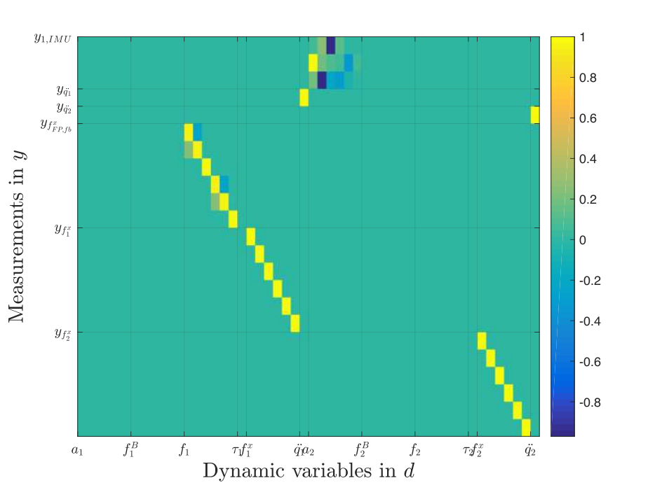
4.3 The Estimation Problem Formulation
| (4.22) |
| (4.23) |
The bottom part of (4.22) represents the constraints equation in (4.5), while the upper part contains the information coming from the, possibly noisy or redundant, sensors. It is possible to compute the whole-body dynamics estimation by solving the system in . The assumption on the rank in (4.23) guarantees that the available measurements give enough constraints on .
The novelty of the framework lies in moving away from the classical approach by replacing RNEA boundary conditions with measurements coming from sensors. Within this new framework, there are situations in which the system is overdetermined and an exact solution does not exist. An ‘approximated’ solution can be obtained only by making some additional hypothesis. If there is a valid reason to assume that all the constraints have equal relevance and all measurements the same accuracy, one possible approach is to solve (4.22) in the ordinary least-squares sense, by using a Moore-Penrose pseudoinverse. Otherwise, if we have good reasons for weighting differently the constraints and the sensors readings, we can use the weighted pseudoinverse to obtain a weighted least-squares solution. However, finding proper weights might be not an easy task.
In this thesis a different choice is performed: given the prior knowledge of the measurements and the prior information about the constraints of the model, the estimation of is framed in a Gaussian domain by means of a maximum-a-posteriori estimator.
4.4 Probabilistic Preliminaries
Since the estimation problem solution is framed in a Gaussian domain, some basic notations related to the probability theory are here recalled.
- •
Given a stochastic variable , let be its probability density distribution and the conditional probability distribution of given the assumption that another stochastic variable has occurred.
- •
Given and , let be their joint probability distribution.
- •
If is associated to a deterministic function , let be the expected value of w.r.t. . Let be the mean of , i.e., and the covariance associated to , such that .
- •
Given a multivariate Gaussian distribution , expressed with the notation
(4.24) its probability density function (PDF) is
(4.25) where denotes the determinant of the matrix . It is worth noting that when in a multivariate normal distribution the covariance is not a full-rank matrix, then the distribution is degenerate and does not have a density. In order to avoid the drawback, it can be useful to restrict the problem on a subset of such that the covariance matrix for this subset is positive definite.
4.5 The Maximum-A-Posteriori Solution
The Maximum-A-Posteriori (MAP) estimator is here adopted as a tool for computing an estimation of the vector and therefore the solution of (4.22). The MAP algorithm can be interpreted as a way for choosing a weighted pseudoinverse according to the reliability of the available measurements.
The first assumption for adopting the MAP approach is to consider the vector of dynamics variables and the vector of the measurements as two stochastic variables with Gaussian distributions. The estimation problem can be summarized as follows.
Since the normal distributions and are jointly Gaussian, the conditional probability distribution is such that
| (4.27) |
In the following computation, the term is negligible since it does not depend on . This is the reason of the proportionality between the conditional probability distribution and the joint distribution in (4.26). Hereafter each term in (4.27) is computed separately to obtain the final analytical solution. For the sake of simplicity, dependencies are omitted in the computations.
Computation of
Let us first give an expression for the conditional PDF :
| (4.28) | |||||
which implicitly makes the assumption that the measurements equation (4.14) is affected by a Gaussian noise with zero mean and covariance .
Computation of
Define now a PDF for the normal distribution . By pursuing the same methodology, we would like to write its distribution in the following form
| (4.29) |
such that the PDF
| (4.30) |
taking into account constraints of Equation (4.5) with .
However, this intuitive choice leads to a degenerate normal distribution and a regularization term is needed. For example, if we have a Gaussian prior knowledge on in the form of distribution, we can reformulate Equation (4.29) as follows:
| (4.31) |
such that (4.30) becomes
| (4.32) | |||||
where the covariance and the mean are, respectively,
| (4.33a) | |||||
| (4.33b) | |||||
The role of is to establish how much the dynamic model (4.5) should be considered correct. The quantities and , instead, define the Gaussian prior distribution on (namely, the regularization term).
Computation of
By combining Equations (4.28) and (4.32) we are now ready to give a new formulation of the estimation problem for the conditional PDF of given , i.e.,
| (4.34) | |||||
with covariance matrix and mean as follows:
| (4.35a) | |||||
| (4.35b) | |||||
Moreover, in the Gaussian case the MAP solution coincides with the mean of the PDF yielding to:
| (4.36) |
4.5.1 The Cholesky Decomposition
Computations for (4.36) can be performed in several ways but computationally cost-efficient solutions need to exploit the sparsity in the matrices and . The solution is here retrieved by applying the Cholesky decomposition. The Cholesky decomposition is mainly used for the numerical solution of systems expressed in the form. This approach allows to decompose the generic symmetric44 4 The Cholesky decomposition embraces the widest case of Hermitian matrices. For the MAP case all the entries of the matrix , thus the Hermitian coincides exactly with its transpose., positive-definite matrix into a product of a couple of triangular matrices (a lower triangular and its transpose), such that .
When is a sparse matrix (i.e., the most of its entries are zero), it is convenient to compute a heuristic permutation matrix for sparsing , such that, . This speeds up remarkably the time of the execution for computing the system solution and the computational cost55 5 The computational cost is considered as the amount of the operations performed during an algorithm execution. It is a parameter to define how the cost scales with the size of the problem. For example, in the case of a matrix related operation, the syntax means that the algorithm has a computational complexity that grows proportionally to (e.g., the complexity of a matrix inversion). decreases passing from a Cholesky to a sparse Cholesky decomposition ().
In the Algorithms 2 and 3, the pseudocodes for computing the solutions (4.33b) and (4.35b) via sparse Cholesky method are shown, respectively. For the sake of simplicity, they were here split into two different algorithms. Clearly, in the code computation they represent a whole algorithm since the solution (4.33b) is mandatorily required for computing (4.35b).
Both the algorithms require the pre-computation of the permutation matrix through the Matlab chol built-in function. Moreover, it is important to note that, even though the algorithm currently does not work in this way, in lines , it would be useful to re-order the matrix (accordingly to the permutation matrix structure) before the step.
4.6 Considerations on the Estimator Choice
In this Section some considerations on the choice of the MAP estimator are made. The accuracy of the estimation heavily depends on the adopted estimator and therefore a detailed description is needed.
4.6.1 Linear Estimator for Jointly Gaussian Vectors
Let , be two random Gaussian vectors with distributions
| (4.37) |
respectively, and jointly Gaussian, i.e.,
| (4.38) |
where the terms and represent the jointly covariance matrices.
Consider now the following estimation problem.
The time has now come to choose the proper form of the estimator . Let us start with considering a minimum mean square error (MMSE) estimator of that is a function which minimizes the mean square error (MSE), i.e., the trace of the error covariance matrix, such that
| (4.39) | |||||
See Equation () of (Petersen and Pedersen 2012) for retrieving Equation (4.39).
It is shown in (Oppenheim et al. 2016) (as well as in many other textbooks of probability theory) that the estimator as defined in (4.39) coincides with the expectation of the conditional distribution
| (4.40) |
such as
| (4.41) |
For the Gauss-Markov theorem (Nowak 2011), if and are jointly Gaussian random vectors with the distribution in (4.38), then the conditional distribution of given is
| (4.42) |
This yields to a new formulation that identifies the estimator , such that
| (4.43a) | |||||
| (4.43b) | |||||
where (4.43a) is the mean and (4.43b) is the covariance associated to the estimator. According to the Gauss-Markov theorem, Equation (4.43a) is a linear function of and in this case the MMSE estimator is said to be linear. In many cases, it is difficult to determine the analytical expression of the MMSE estimator. A widely used tradeoff is to restrict the estimator to be a linear (i.e., linear plus a constant) function of , and to choose the linear relationship in order to minimize the MSE (Oppenheim and Verghese 2010). The resulting estimator is called the linear minimum mean square error (LMMSE) estimator.
4.6.2 Linear Estimator for Linear Regressors
Let us suppose now to consider the following linear regressor model:
| (4.44) |
where
| (4.45) |
are the distributions of the Gaussian variable and of the error , respectively. This straightforwardly yields to
| (4.46) |
being and the mean and the covariance of the regressor model, respectively. Also in this case we can consider the same jointly Gaussian situation as in (4.38), where now:
| (4.47) |
Given that, the set of Equations (4.43) become
| (4.48b) | |||||
This formulation is useful to understand what happens to the solution when the variable (i.e., the prior in our algorithm) is very reliable. This yields to and therefore to
| (4.49a) | |||||
| (4.49b) | |||||
Another equivalent representation can be provided by applying the Woodbury identities:
- •
to (4.48) (see Equation () in (Petersen and Pedersen 2012) or in (Golub and Van Loan 1996), Chapter )
(4.50) - •
to (4.48b) (see Equation () in (Petersen and Pedersen 2012))
(4.51)
Given (4.50) and (4.51), Equations (4.48) can be written as
| (4.52b) | |||||
Equation (4.52) clearly shows that the solution is the weighted sum of (i.e., the mean of the prior in our algorithm) and the variable (i.e., the measurements vector in our algorithm). The second formulation is convenient to understand what happens in case of is very unreliable (). In this case, the solution is mainly relying on , such that
| (4.53a) | |||||
| (4.53b) | |||||
4.6.3 Generalized Least-Squares Estimator
In this Section it is shown that the linear estimator solution of the problem in Section 4.6.1 coincides with the solution of the generalized66 6 The generalized least-square problem is a weighted least-squares where is a non-diagonal matrix, but still symmetric and positive-definite. least-squares (GLS) problem.
Define the following GLS problem for the system in the form :
| (4.54) | |||||
Thanks to Cholesky factorization (see Section 4.5.1), if (symmetric77 7 Indeed here it is required an Hertian matrix , but the case of only real entries yields to .) and (positive-definite), it is always possible the following decomposition:
| (4.55) |
where is an upper triangular matrix. Thus in (4.54),
| (4.56) | |||||
Consider in our specific case and , such that in (4.54)
| (4.57) | |||||
4.6.4 The MAP Estimator
The solution (4.57) is written in the form of the MAP solution (4.35). Thus solving the problem in (4.26) is equivalent to solve a generalized least-squares problem (4.57). Because of this, the MAP problem can be written in the following form:
The importance of the Equation (4.6.4) is two-fold:
- )
it shows clearly the role of each part in the estimation of : the contribution of the dynamic constraints weighted by , the contribution coming from the sensor readings weighted by and the contribution due to the prior on weighted by ;
- )
it provides the form of and for the solution in (4.54):
(4.59)
If we prefer, Equation (4.6.4) can be written in the following form:
| (4.60) |
where can be seen as a regularization term in shaping the measurements equation.
Chapter 5 Software Implementation and Algorithm Validation
- -
If an experiment works, something has gone wrong.
- -
In any collection of data, the figure most obviously correct, beyond all need of checking, is the mistake.
Finagle’s laws, Arthur Block
This Chapter presents the software implementation of the MAP solution and several offline validation procedures to assess the effectiveness of the presented estimation algorithm. Since the sensors play a paramount role in the analysis, they will be detailed described in a dedicated section. A new type of wearable force sensing is also introduced in this Chapter and an investigation for its validation w.r.t. the force gold standard is provided to the reader.
5.1 MAP Software Implementation
In this Section the software architecture of the MAP framework is presented (see pipeline in Figure 5.1). It was implemented in Matlab and created specifically for offline validations. The code related to the MAP offline computation is hosted on GitHub in a dedicated public repository (MAPest 2016). The starting point of the analysis consists in the IMUs readings. Kinematic data are parsed into a compatible Matlab format and then processed as in the following steps.
- •
Computation of the position of each sensor in the suit w.r.t. the attached link. Xsens does not provide directly this information as output, therefore it is necessary to compute it through the estimation Algorithm 1 (Chapter 3). This step is mandatory since sensors position has to be encoded in the non-standard extension of the URDF (see Section B.1 of Appendix B). It is worth remarking that, at this stage, a URDF template exists, built according to the human whole-body modelling in Figure B.2. The dimension of the URDF elements (cylinders, parallelepipeds and spheres) is estimated from IMUs data by making in this way the model scalable with the subject proportions. This is possible thanks to the Xsens trajectories acquisition of ‘fictitious’ markers positioned at several anatomical known bony landmarks.
- •
Computation of the Inverse Kinematics (IK) by means of the OpenSim specific toolbox (OpenSim) (Delp et al. 2007) that solves a weighted least-squares problem for obtaining the joint angles . This is possible thanks to an OpenSim (OSIM) template previously built in order to match with the URDF model and a .trc file containing the markers trajectories acquired by the Xsens system, (see Appendix C). Joint velocities and accelerations are computed by using a weighted sum of moving windows of elements with a third-order polynomial Savitzky-Golay filtering (Savitzky and Golay 1964).
- •
Extraction of the IMUs linear acceleration readings for filling the measurements vector .
All the above-listed points are used to obtain Equation (4.14) for the measurements. They are typically kinematic readings, force sensing data (e.g., the ground reaction forces but in general the external forces acting on the model links) and joint accelerations that are here considered as acquired from a class of ‘fictitious’ DoF-acceleration sensors. By exploiting the information coming from the model and the state, the pipeline block of the MAP computation provides the estimation of given (see Algorithm 3, Chapter 4). It is worth to highlight that Figure 5.1 does not refer to the temporal aspect of the data flow. For a better understanding of the steps sequentiality refer to the Algorithm 4, where a situation with subjects performing different tasks is considered.
5.2 Experimental Sensor Setup
5.2.1 Motion Capture
The full-body motion capture tracking of the human is retrieved by a Xsens wearable lycra suit in which wired body-mounted IMUs (Figures 5.2(a), 5.2(b)) are located in the upper legs, lower legs, upper arms, lower arms, the pelvis, the sternum, the shoulders and the head. All the IMUs are connected to the Xbus Masters (mounted on the back of the subject) that is in charge of synchronizing the sensor readings, providing them with power and handling the wireless communication with a laptop. The wireless connection is guaranteed by an external Access Point connected via Ethernet to a laptop. See Figure 5.2(c) for the Xsens motion capture tracking setup. The output of this system is a XML-like file with the kinematic variables of the subject who is wearing the suit, according with the Xsens body modelling (Figure 3.1).


5.2.2 Ground Reaction Forces Tracking
For tracking the human ground reaction forces a new sensing shoes technology was used. By starting from a Xsens original design (Schepers et al. 2007), the ftShoes wearable technology is a prototype recently developed at Istituto Italiano di Tecnologia for measuring the human ground reaction forces. It consists of a pair of shoes instrumented with four Force/Torque (F/T) sensors (Figures 5.3(a), 5.3(b)) applied at the bottom of both soles. Each shoe has two F/T sensors positioned at the heel and the forefoot, respectively, and in turn each sensor is comprised in between two metallic thin plates, thus they can be considered independent w.r.t. each other. Each human foot is placed in the ftShoe as in Figure 5.3(c).


5.3 Data Analysis
Data for the algorithm validation were collected at University of Waterloo (ON, Canada). The setup encompassed the Xsens wearable suit (in the look-and-hoop strap version) for the human motion tracking , the ftShoes prototype for the ground reaction computation. Two portable AMTI force plates and a printed fixture of the shoes to be applied on the force plates (Figure 5.5(a)) were additionally required for the shoes validation.
Five healthy subjects (Table 5.1) were asked to wear the sensorized suit and the ftShoes and to perform on the force plates different tasks, with the feet aligned to the printed fixture (as Figure 5.5(b)). The tasks selected for this analysis are listed here as follows and shown in Figure 5.4:
Kinematic data were acquired at a frequency of , force plates and ftShoes data at . The synchronization between the motion capture system and the force plates was guaranteed by a synch station provided by Xsens. Readings from the shoes11 1 ftShoes readings are obtained through YARP, see in chapter Section 6.1. were synchronized by code. Data with different acquisition rates were linearly interpolated before being processed.


| Subject | Gender | Age | Height [] | Mass [] |
|---|---|---|---|---|
| S1 | M | |||
| S2 | F | |||
| S3 | M | |||
| S4 | M | |||
| S5 | M |
5.3.1 ftShoes Validation
The Section reports the analysis for the validation of the new technology w.r.t. the gold standard in ground reaction force measurements (i.e., the force plates). The analysis required to express both readings in a common reference frame (e.g., the human foot frame22 2 IMUs readings have been used here for retrieving the position of each foot w.r.t. the reference frame of the related ftShoe/force plate.).
A Root Mean Square Error (RMSE) analysis (Table 5.2) has been performed for the above described dataset, for validating the three components of the forces (, ,) and moments (, , ). Figure 5.6 shows the forces (on the left column) and moments (on the right column) for validating the left ftShoe reading (in human left foot frame) w.r.t. the gold standard provided by its coupled force plate FP1, for subject S1, tasks T1-T2. Similarly, Figure 5.7 validates the right ftShoe w.r.t. the force plate FP2, for the same subject, in the same tasks.
The RMSE values are in general very low denoting a good matching of each shoe signal w.r.t. the related force plate. Despite some values (highlighted in red) seem to provide a worst estimation of the forces, they are anyway considered acceptable from the force plate datasheet33 3 From AMTI datasheet: by considering an error of on the full scale due to a combination of hysteresis and non-linearity noises and a subject standard weight of [], the error on the forces could be quantified as []. Similarly for the moment error [].. Another important source of error could be attributed to fact that the shoes are not rigidly attached to the force plates. It is worth noting that, even if explicitly required, the subject did not hold his feet fixed on the fixture (e.g., some tasks implicitly caused slippery conditions), while the analysis is completely based on this strong assumption (i.e., constant transformation between the ftShoes/force plates origins).


| Subject | Task | FP1 - left ftShoe | FP2 - right ftShoe | ||||||||||
|---|---|---|---|---|---|---|---|---|---|---|---|---|---|
| S1 | T1 | ||||||||||||
| T2 | |||||||||||||
| S2 | T1 | ||||||||||||
| T2 | |||||||||||||
| S3 | T1 | ||||||||||||
| T2 | |||||||||||||
| S4 | T1 | ||||||||||||
| T2 | |||||||||||||
| S5 | T1 | ||||||||||||
| T2 | |||||||||||||
5.3.2 Estimation of Human Variables
The MAP algorithm is a tool for estimating quantities related to the joints and links of the human model. It is worth remarking that the vector (the solution (4.35b)) contains variables that can be directly measured (, ) and variables that can not be directly measured in humans (, , ) but only estimated through the algorithm.
The MAP algorithm represents, in a sense, the probabilistic way to estimate those quantities for which a direct measure does not exist. We consider the goodness in the estimation of the measurable quantities as a parameter of reliability of the method in estimating those variables that are no directly measurable. The leading idea is to compare the same variables (measured and then estimated) in order to prove the quality of the proposed algorithm.
Subjects of Table 5.1 were asked to perform tasks T1 and T2 equipped with the Xsens suit for the motion tracking and the ftShoes prototype for computing the ground reaction forces.
Xsens data were acquired at through the MVN Studio software, ftShoes data at through the YARP driver. Data were synchnonized and downsampled in post-processing phase by means of Matlab. A -DoF model template was used both for the URDF and for the OpenSim model, (). The IK was computed by using the OpenSim API for Matlab and a Savitzky-Golay filtering (-th order, -elements moving window) was used for retrieving joint velocities and accelerations . The MAP settings were tuned as follows: (i.e., no reliable prior on vector ), (i.e., high reliable prior on the dynamic model), composed of each sensor variance submatrix (IMUs , joint acceleration , external forces on the feet and on the other links of the model ).
The analysis shows the comparison between the measure and the estimation for the external forces, linear accelerations and joint accelerations of certain links/joints of the model. Their choice was task-driven by considering those links/joints mainly involved in the tasks. The analysis has been performed for all the subjects in Table 5.1 along with a RMSE investigation for the external forces (Table 5.3), the linear accelerations (Table 5.4) and the joint accelerations (Table 5.5). However, the following figures refer to one subject (i.e., S2) and they have to be interpreted in the following way: the three columns are the x-y-z components; the rows are related to the link/joint chosen for the evaluation. Blank plots mean that there is not a related quantity for that component (depending on the joint DoFs).
Figure 5.8 shows the comparison between the external force [] measured (in red) and estimated by the algorithm (in blue) for the right foot44 4 The similar analysis on the left foot is not retrieved since the left foot is the fixed base of the model. In general, the iDynTree library (Nori et al. 2015b) used here for describing the dynamics of the model does not support the application of any kind of sensor on the fixed base and therefore neither the estimation of its dynamics.. Figure 5.9 shows the comparison between the linear acceleration [] measured by sensors (in red) and estimated quantity (in blue) by the algorithm for right upper arm, forearm and hand links, respectively, in the tasks T1 (on top) and T2 (on bottom). Figure 5.10 shows the same analysis for the related left links. Similarly, the comparison between the joint acceleration [] (assumed to be) measured by the class of ‘fictitious’ DoF-acceleration sensors (in red) and the related estimation (in blue) via MAP is shown for the right (in Figure 5.11) and for the left (in Figure 5.12) shoulder, elbow and wrist joints, respectively, for T1 (on top) and T2 (on bottom).
![[Uncaptioned image]](1912.01136v1/legend.png)
![[Uncaptioned image]](1912.01136v1/fext_comparison.png)
| Subject | Task | rightFoot | |
|---|---|---|---|
| S1 | T1 | ||
| T2 | |||
| S2 | T1 | ||
| T2 | |||
| S3 | T1 | ||
| T2 | |||
| S4 | T1 | ||
| T2 | |||
| S5 | T1 | ||
| T2 | |||
![[Uncaptioned image]](1912.01136v1/x1.png)
![[Uncaptioned image]](1912.01136v1/acc_dx_comparison.png)
![[Uncaptioned image]](1912.01136v1/acc_sx_comparison.png)
| Subject | Task | rightUpperArm | rightForeArm | rightHand | leftUpperArm | leftForeArm | leftHand | |
|---|---|---|---|---|---|---|---|---|
| S1 | T1 | |||||||
| T2 | ||||||||
| S2 | T1 | |||||||
| T2 | ||||||||
| S3 | T1 | |||||||
| T2 | ||||||||
| S4 | T1 | |||||||
| T2 | ||||||||
| S5 | T1 | |||||||
| T2 | ||||||||
![[Uncaptioned image]](1912.01136v1/x2.png)
![[Uncaptioned image]](1912.01136v1/ddq_dx_comparison.png)
![[Uncaptioned image]](1912.01136v1/ddq_sx_comparison.png)
| Subject | Task | rightShoulder | rightElbow | rightWrist | leftShoulder | leftElbow | leftWrist | |
|---|---|---|---|---|---|---|---|---|
| S1 | T1 | |||||||
| T2 | ||||||||
| S2 | T1 | |||||||
| T2 | ||||||||
| S3 | T1 | |||||||
| T2 | ||||||||
| S4 | T1 | |||||||
| T2 | ||||||||
| S5 | T1 | |||||||
| T2 | ||||||||
Hereafter, the human joint torque estimated by the MAP algorithm. No direct comparison with the related measured quantity is possible in this case.
5.3.3 Incremental Sensor Fusion Analysis
As previously said, the novelty of the MAP framework consists in replacing the classical RNEA boundary conditions with readings coming from different types of sensors. In this Section, we discuss the benefits of the multi-sensor data fusion for solving the estimation problem by characterizing the effects of the data fusion on the covariance of the estimator. The benefit of the MAP is such that the more sensors we use in the estimation, the better the estimation itself will be. Let us consider writing Equations (4.33a) and (4.35a) in a more compact form, such as
| (5.1) |
Let us assume multiple statistically independent measurements
this yields to a diagonal structure for the matrix . Thus, we have:
| (5.3) | |||||
With an abuse of notation, let be the estimator which exploits all the measurements from up to . The addition of each measurement induces changes into the associated covariance matrix according to the following recursive equation:
| (5.4) |
where, for , the initial condition is
| (5.5) |
A situation of two sets of measurements equations is here evaluated for the subjects in Table 5.1, for tasks T1 and T2. In particular, the measurements equation (4.14) is built for two different cases:
| (5.6a) | |||||
| (5.6b) | |||||
The MAP algorithm is performed twice by including as set of sensors firstly Equation (5.6a) and then Equation (5.6b). The attempt is to prove that, by adding (e.g., increasing) progressively different sensors data, the variance associated to the estimated dynamic variables consequently decreases at each MAP computation, by making the estimation more reliable. By passing progressively from CASE 1 to CASE 2 the variance associated to the torques decreases. Figure 5.17 shows the decreasing behaviour of the -subjects mean torque variances from CASE 1 (in orange) to CASE 2 (in violet) for both left and right ankle, hip joints, respectively and L5S1, L4L3, L1T12 joints. The two plots are for the tasks T1 (5.17(a)) and T2 (5.17(b)).
The variance values at the ankles do not change significantly among the two cases since the ankle torque estimation depends mostly on the readings of the ftShoes that are included in both of them. Conversely, an ever-growing decreasing behaviour is present starting from the values associated to the hips towards the L1T12 joint on the torso. This because as we are considering joints always further apart from the feet, the ftShoes contribution to the estimation has a lower weight than at the feet while the contribution of the IMUs becomes more important (i.e, weights more). In Table 5.6 detailed values of the analysis per each subject are reported.
| Subject | Task | CASE | lAnkle | rAnkle | lHip | rHip | L5S1 | L4L3 | L1T12 |
|---|---|---|---|---|---|---|---|---|---|
| S1 | T1 | ||||||||
| T2 | |||||||||
| S2 | T1 | ||||||||
| T2 | |||||||||
| S3 | T1 | ||||||||
| T2 | |||||||||
| S4 | T1 | ||||||||
| T2 | |||||||||
| S5 | T1 | ||||||||
| T2 | |||||||||
5.4 An Experiment with the iCub
The analysis, performed in the previous section, is here shown in a variant that encompasses the robot iCub. Data were collected at Istituto Italiano di Tecnologia, on a -DoF human model (). The experimental setup encompassed the Xsens suit for the motion tracking, two standard AMTI OR force platforms to acquire the ground reaction wrenches, the F/T sensors of the robot arms. ftShoes were not used in the experiment since they did not exist at that time. Kinematic data were acquired at a frequency of . Each platform acquired a sample at a frequency of by using AMTI acquisition units.
Experiments were conducted on the iCub (Metta et al. 2010), a full-body humanoid robot with DoFs: in the head, in each arm, in the torso and per each leg. The iCub is endowed with whole-body distributed F/T sensors, accelerometers, gyroscopes and tactile sensors. Specifically, the limbs are equipped with six F/T sensors placed in the upper arms, in the upper legs and in the ankles. Internal joint torques and external wrenches are estimated through a whole-body estimation algorithm (Nori et al. 2015b). Robot data were collected at a frequency of .
Ten healthy adult subjects (as in Table 5.7) have been recruited for the experimental session. Each subject was asked to wear the Xsens suit and to stand on the force plates by positioning one foot per platform. The robot was located in front of the subject facing him at a known position w.r.t. the human foot location (Figure 5.18(a)). The mutual feet position was fixed for all the trials and defined by a printed fixture located under both feet (Figure 5.18(b)) The interaction implied that the human grasped and pushed down both the robot arms while performing a bowing task (Figure 5.19).
As in Section 5.3.2, even here the MAP algorithm was able to estimate for all the links/joints in the model. As in the previous dataset, the MAP results are here shown for one subject (i.e., S1). Figure 5.20(a) shows the comparison for the external forces measured (in red) and estimated (in blue) for the right foot55 5 No left foot as previously motivated. and for both the human hands since during the interaction there are forces acting on them. The same comparison concerning the linear acceleration for the right foot, upper leg and hand, respectively, is shown in Figure 5.20(b). Similar analysis in Figure 5.21(a) for the joint acceleration, for the right ankle and the hips. Again here, like in the previous case, the MAP algorithm is able to give us a suitable estimation of the human joint torques, Figure 5.21(b).
| Subject | Gender | Age | Height [] | Mass [] |
|---|---|---|---|---|
| S1 | F | |||
| S2 | F | |||
| S3 | M | |||
| S4 | M | |||
| S5 | F | |||
| S6 | F | |||
| S7 | F | |||
| S8 | F | |||
| S9 | M | |||
| S10 | M |


![[Uncaptioned image]](1912.01136v1/legendSinStd.png)


As in the Section 5.3.3 analysis, an investigation by adding progressively different sensors has been done on the MAP computation. The set of measurements equation (4.14) is here composed as follows:
| (5.7a) | |||||
| (5.7b) | |||||
| (5.7c) | |||||
Even in this case the analysis reveals the important decreasing behaviour as in Figure 5.17. By passing progressively from CASE 1 to CASE 3 the variance associated to the -subjects mean torques decreases, Figure 5.22. Again, the variance values on the ankles do not change significantly among the three configurations since the ankles torque estimation depends mostly on the contribution of the force plates that are included in all the three cases. And for the same previous reason, the decreasing behaviour becomes to be evident at the hips since the torque estimation at the hips is affected by the complete set of sensors (i.e., contribution of the force plates weights lower, contribution of IMUs + F/T iCub sensors weights more).
5.4.1 MAP vs. OpenSim Dynamics Estimation
To test the quality of our estimation w.r.t. a ground-truth tool, one subject of Table 5.7 was asked to perform four repetitions of the bowing task in two different configurations, i.e., with and without an additional mass of roughly positioned in correspondence of the torso center of mass. The MAP computation was performed by considering the following cases as algorithm inputs (see Table 5.8).
| CASE A | CASE B | |
| URDF model | without | without |
| measurements | with | without |
| estimation |
In both the cases the analysis is performed with the same URDF model of the subject. In order to highlight a lower reliability for the CASE A, it is assigned a value to equal to (different from the value assigned for the CASE B).
By exploiting the linearity property of the system we consider the following expression for the torques:
| (5.8) |
where is the theoretical torque due to the additional positioned on the torso66 6 We consider a simple -DoF system (see (Latella et al. 2016)) in which the position of and the hip joint angle are known.. Figure 5.23 shows the mean and the standard deviation of the torque estimation at the hips (i.e., the sum of the torque estimated at each hip) by means of the MAP algorithm (Figure 5.23(a)) and the OpenSim ID toolbox (Figure 5.23(b)), respectively.
Given Equation (5.8), it is possible to retrieve the error on the estimation due to the presence of the weight :
| (5.9) |
Equation (5.9) has been computed for both the estimators in order to evaluate its effectiveness w.r.t the modelling errors. The error is higher in OpenSim ID computation (6.45 ) than in the MAP estimation (3.69 ) since OpenSim does not offer the possibility of setting the model reliability in the computation. This highlights that the MAP algorithm is a method more robust to the modelling errors since it gives the possibility of weighting the reliability of the model by properly tuning the related covariance matrix.


Chapter 6 Towards the Real-Time Human Dynamics Estimation
The Scientist must set in order. Science is built up with facts, as a house is with stones. But a collection of facts is no more a science than a heap of stones is a house.
Henri Poincaré
In this Chapter, a first attempt to aim at advancing the current state of the art in pHRI is presented through the design of an estimation tool for monitoring the dynamics of the human in a real-time domain. From a theoretical point of view, the online design does not differ from the version implemented in the previous chapter. However the logic in which input data have to be acquired and the way in which they have to be processed are completely different in the real-time context. Here the idea is to exploit a middleware already developed for the robot iCub to perform the online human dynamics estimation. To this scope the software implementation in Figure 5.1 was revisited and modified accordingly.
All the software related to this Chapter has been released as an open source-code and it is hosted on GitHub in the Robotology organization (HDE 2017).
6.1 YARP Middleware for the Human Framework
YARP (Yet Another Robot Platform) is a middleware developed at Istituto Italiano di Tecnologia (Metta et al. 2006). It is a C++ platform embedding libraries, protocols and tools, written for interfacing humanoid robots. YARP is mainly used to minimize the effort in the infrastructure-level software development by facilitating the code reusability and modularity.
YARP allows to split the algorithm for the estimation of the human dynamics into different modules by ensuring communication and connection between them but preserving, in the meanwhile, their independence (Romano et al. 2017). The algorithm, represented in Figure 5.1 for offline evaluations, is hereafter structured into modules (in Figure 6.1) in order to fit the online requirements.
The human-state-provider Module
As suggested by the name, the module has to provide in real-time the human state . A pre-built URDF model of the human and the Xsens motion capture data (coming here from a YARP driver) are the inputs of the module. The information coming from the motion capture system has to be converted in a representation compatible with our human dynamic model represented in Equation (4.22), as follows.
Let and be two links coupled by a joint. If , are the pose of the links w.r.t. a generic inertial frame in the original human model (i.e., the Xsens model) and , the pose of the same quantities in our dynamic model, we can use IK to map the links pose to the configuration . The relative pose is for the original model, for our model. The module solves a nonlinear optimization problem, such as
| (6.1) |
The solution of the problem (6.1) is that value of that minimizes the error function in the joint limits range .
To compute the velocity , the module reads from the Xsens the angular velocities , and computes the relative angular velocity of the two links . Our model velocity is then computed by inverting the following relation:
| (6.2) |
where is the relative Jacobian of the link w.r.t. the link and is the angular velocity of the link w.r.t. the link of our dynamic model. Since in general , Equation (6.2) is solved in the least-squares sense, such that
| (6.3) |
For each pair of coupled links , the human-state-provider is in charge of computing the mapping procedure . This formulation is quite generic and allows to handle models of different complexity.
The human-forces-provider Module
The module is composed of two interfaces. The first interface is in charge of reading forces coming from different YARP-based devices (force plates or ftShoes) and from YARP ports (the iCub, in case of pHRI). The second interface transforms force readings into D force vectors expressed in human reference frames, as required from the vector of measurements . The proper force transformation requires that the pose of the human w.r.t. the force plates and the robot is a known quantity.
The human-dynamics-estimator Module
The module provides the final estimation for the vector given as inputs the previous two modules output data. In order to proper cluster data into vector, it needs the human state and the forces readings both expressed in humans frames. Then, together with the human state and some information extracted from the URDF model, the module launches the MAP algorithm with the Cholesky factorization.
YARP allows to visualize the real-time human dynamics estimation (whether a pHRI is occurring or not) by means of some structured modules and a ROS-based visualizer (gray part in the Figure 6.1). The human-viz module in composed of different YARP submodules that are in charge of reading information from the Xsens system, the human state , the estimated vector , and of publishing information to be sent to the visualization tool in the form of ROS-topic messages. ROS messages (including those coming from the human-forces-provider module) are visualized in the toolkit RViz (Kam et al. 2015). The advantage in adopting this tool is due to its versatility and agnosticism to the type of the data structure or algorithm.
At this preliminary stage, we observed that is a sufficient frequency for the outputs of the human-forces-provider and the human-dynamics-estimator modules; for obtaining a suitable output of the human-state-provider module. The last frequency is strongly dependent on the type of optimization solver used in computing the IK.
6.2 Towards the Online Estimation
A preliminary investigation on the online algorithm estimation has been done. Similarly to the experimental setup in Figure 5.19, a subject was asked to wear the suit and the ftShoes and to interact with the iCub through a pushing bowing. The estimation vector was here online computed by the YARP infrastructure in Figure 6.1. Figure 6.2(a) shows very preliminary results of three consecutive pHRI bowings. It shows the comparison between the external forces transformed in human frames by the human-forces-provider module (in red) and the same forces as estimated in by the human-dynamics-estimator module (in blue). The same analysis has been done for four repetitions of pHRI squat task, Figure 6.2(b). It is important remarking that these preliminary results are relying only on the forces measurements (i.e., no IMUs or joint accelerations on vector ). Although they are very promising, further investigations are required in the very next future.
In addition to providing a visual feedback to the estimation, the visualizer gives us an important information about how much the human joint effort is. The joint torques (estimated via MAP) are represented with spheres whose colour is an indicator of the ‘effort’: in a gray scale, a light sphere means a high effort, a dark sphere a minor effort. Figure 6.3 shows three different pHRI tasks with their real-time visualizations, for a bowing, a squat task, a task in which the human is helping the robot to stand up from a rigid support, respectively. At the current stage, any kind of pHRI can be visualized in the real-time framework as long as it obeys the initial assumptions, (i.e., fixed base and rigid contact conditions).


Chapter 7 The human-in-the-loop Concept
Without haste, but without rest.
Wolfgang von Goethe
This Chapter discusses the possibility to extend the human dynamics estimation framework to a new framework that encompasses an active collaboration with a robot. The human-in-the-loop concept implies that the human agent is collaborating with a torque-controlled robot that is able to exploit the human collaboration (in term of human dynamics) to achieve its control objective. The dyadic interaction yields to a bidirectional contribute:
from the human side, it is mandatory to exploit the contact forces measured during the interaction through the robot for computing the human dynamics;
from the robot side, it is mandatory to exploit the information coming from the human dynamics in order to synthesize a new control objective for taking advantage from the human help.
The partner-aware robot control is out of the scope of this thesis since it still has to be developed in the very next future. However, the Chapter introduces the theoretical background on which the control theory will lay its foundations.
Within this context, the framework has to be applied to a new coupled system composed by the human and the robot. The two agents maintain their own modelling (possibly in a comparable formalism) but new assumptions on the holonomic constraints have to be properly done.
7.1 Coupled System Modelling
Consider an interaction scenario with two agents: the human and the robot (see a generic scenario in Figure 7.1). Consider also to express the two systems with the formalism adopted for humanoid robots. The advantage of this choice is straightforward since it allows to handle both the systems with the same mathematical tool. In this domain, the application of the floating-base formalism in Section (2.5.2) leads to two sets of motion equations for the two systems, such that
| (7.1a) | |||||
| (7.1b) | |||||
where the physical meaning of each term is defined in Table 7.1.
Assume that the human is subject to external forces . These forces are composed of two subsets: the forces applied to the system by the environment (e.g., from the ground), and the forces due to the dyadic interaction with the other agent, such that
| (7.2) |
Similarly for the robot agent, there are two types of forces and , thus
| (7.3) |
Since the two systems are interacting with the environment independently from each other and from the mutual interaction, there is not any relation between the forces that the environment applies to each system (namely, and ). Conversely, when the contact occurs, the interaction implies a holonomic relation between and .
| Terms in Equations (7.1) | Human | Robot |
|---|---|---|
| Internal DoFs | ||
| Mass matrix | ||
| Coriolis effects matrix | ||
| Gravity bias | ||
| Configuration | ||
| Velocity | ||
| Torque | ||
| Jacobian | ||
| Force∗ |
7.2 Rigid Constraints
Let be a generic inertial frame and define a set of frames
| (7.4) |
associated to the human forces of (7.2), attached to the human links on which the forces are acting. More in detail, frames positions correspond to the point (on the link) of the force application with a z-axis pointing on the direction normal to the contact plane. If we consider a generic element (both for or ), it is always possible to describe the following relation
| (7.5) |
where the Jacobian is the map between the human floating-base velocity and the velocity of the frame attached to the link w.r.t. .
Similarly for the robot, Equation (7.4) becomes
| (7.6) |
and if we consider the generic -th element , thus
| (7.7) |
We can now distinguish between two types of rigid constraints occurring in a pHRI scenario, as represented in Figure 7.1.
1) Environment Holonomic Constraints
If both the systems are rigidly attached to the ground during the interaction (see (a) and (b) in Figure 7.1), it can be assumed that the -th frame in the set (7.4) associated to and the -th frame in the set (7.6) associated to have a constant pose w.r.t. . For the duration of the contact, they have both zero velocity such that
| (7.8a) | |||||
| (7.8b) | |||||
The differentiation of the Equations (7.8) yields to:
| (7.9a) | |||||
| (7.9b) | |||||
where (7.9a) represents the holonomic constraint of the human with the environment and (7.9b) the holonomic constraint of the robot with the environment.
2) Dyadic Interaction Holonomic Constraints
When the two systems mutually interact through a physical contact (see (c.1) and (c.2) in Figure 7.1), the relative transformation between the frames and assumes the following form:
| (7.10) |
where denotes the transformation from the inertial frame to the human frame and from the robot frame to . When is constant, it means that the human and the robot are in contact. The assumption of rigid contact yields to the condition that the relative velocity between and is zero and that they are moving with the same velocity w.r.t. , such as
| (7.11) |
Consider, for the sake of simplicity, a situation in which the two frames and are coincident, thus and Equation (7.11) becomes
| (7.12) |
By substituting Equations (7.5) and (7.7) in (7.12)
| (7.13) |
and differentiating Equation (7.13)
| (7.14) |
| (7.15) |
In general, the pHRI scenario is fully described by the set of the following Equations:
A first investigation into the direction of a reactive pHRI has been done in (Romano et al. 2017). The paper attempts to answer the question “How can we predict human intentions so as to synthesize robot controllers that are aware of and can react to the human presence?” by considering an interaction scenario between a human (equipped with the sensor technology described in the previous chapters) and a human-aware iCub robot. In the paper, the momentum-based balancing controller of the robot has been modified (see Section of the paper) to take into account and exploit the human forces. A task for the robot stand-up from a rigid support has been performed with (as at the bottom of the Figure 6.3 ) and without the human help. Preliminary results show that the robot needs to provide less torque when helped by the human since it is capable to exploit the human assistance.
Chapter 8 Conclusions and Forthcoming Works
Whatever you can do or dream you can, begin it. Boldness has genius, power and magic in it. (Begin it!)
(misattributed to) Wolfgang von Goethe
The understanding of human dynamics and the way in which its contribution can be applied to enhance a physical human-robot interaction are two of the most promising challenges for the scientific community. The ever-growing interest in the topic, mainly aroused in the last two decades, led us to explore and shape the interaction mechanism involved during a physical interaction between humans and robotic machines.
Three years ago, the project call of my Ph.D. course stated the following sentence: […] this research proposal aims at developing a prototype of a force and motion capture system for humans. By bearing in mind the final objective of the project, we really developed that prototype. This thesis describes the design of a novel framework for the simultaneous human whole-body motion tracking and dynamics estimation. However, it puts several questions that have to be tackled in the future if the human estimation will be integrated in the robot control loop to enhance the human-robot interaction.
In this conclusive Chapter, every treated topic in the thesis is recalled together with a discussion of the results and the future developments.
8.1 Discussion
In Chapter 3 we apply the estimation approach to human models described as articulated multi-body systems composed of -DoF revolute joints, by using the classical formalism widespread in robotics (Featherstone 2007). In particular we combined this type of joints to obtain a series of joints with a high number of DoFs ( or ). As a straightforward consequence, the model is composed by real and fake links (see Appendix B). This results in a very big vector (i.e., ) and affects remarkably the computational time. The first intervention will deal with a solution for removing the fake links from the model.
Furthermore, real human joints barely exhibit the pure-axial motion, thus our modelling is only a rough approximation of the complexity exhibited by real-life biomechanical joints. Despite the fact that we chose this joint model for an initial exploration of the method, the proposed algorithm is not limited to this particular choice. In particular the properties of any joint (with an arbitrary number of DoFs) can be encapsulated in an interface where the relative position, velocity and acceleration of the two bodies connected by it are described by arbitrary functions of joint coordinates variables and their derivatives that can then be directly inserted in the equations of the system (4.22). In this way, any kind of joint modelling can be described under this formalism. In the future we plan to generalize the method to arbitrarily complex musculoskeletal models (see a possible inspiring implementation in (Seth et al. 2010)).
Another important investigation will concern the estimation of the human inertial parameters (mass, CoM, inertias). The use of the anthropometric tables is currently the most used tool for estimating such values. Even though the tables allow to scale the model along with the subject, this could be a rough approximation for the non-standard population samples (children, elderly, obese, individual with prostheses) and this is pushing the scientific community towards the development of new alternative ways to estimate these parameters directly from data (Venture et al. 2009), (Robert et al. 2017).
Chapter 4 describes the human dynamics estimation problem by framing the solution in a probabilistic domain by means of a MAP estimator or equivalently a weighted least-squares. The main limitation of the current stage lies in its fixed-base formulation. Even if a mathematical formalism already exists for the floating-base representation (e.g., Equation (2.30)) the existing software tools do not support it yet. The upgrade to a floating-base model is mandatory if we want to test our algorithm in more complex experimental setups where both humans and robots could move while interacting.
Chapter 5 presents a software implementation for the MAP algorithm specifically tailored for Matlab offline validation procedures. The Chapter shows how the algorithm is able to estimate human kinematic and dynamic variables. The estimation capability of the algorithm is validated through a comparison between those variables that can be measured and estimated at the same time. Although Section 5.3 leads to suitable estimations, the method questionability lies the over-reliance of the solution on the chosen measurement covariances. Their initial setting was manually tuned by using datasheet values (when available) and kept constant for all the setups. This may have altered the goodness of the results. The problem equally affects the real-time YARP estimation since, at the current stage, even there the measurement covariances are defined in a fixed initial configuration file. The next forthcoming work goes towards the direction of a sort of data-driven covariance estimation as it is well-known that the measurement covariances may vary when the process is at different operating conditions (Romagnoli and Sánchez 1999). The Expectation-Maximization (EM) algorithm is one solution for the data-driven estimation (Keller et al. 1992) (Chen et al. 1997) (Kulathinal et al. 2002). By starting from a known initial covariance of the measurement (e.g., from the sensor datasheet), the covariance (Equation (4.35a)) could be optimized until the EM does not increase the likelihood anymore.
Chapter 6 endeavours to design a C++ based tool for monitoring the real-time dynamics of a human being physically involved in a collaborative task with a robot. This Chapter, in a sense, describes the real-time evolution of the previous offline framework and proposes a preliminary validation analysis with very promising results. The real-time context automatically yields to a different way for retrieving the human state and the joint accelerations w.r.t. the offline case. Currently, a straightforward way for computing and from data has been already implemented in Section 6.1. However, we are still investigating on the real-time way for obtaining . Some solutions are suggested in (van den Bogert et al. 2013) and in the GitHub repository (RTbiomechanics).
For the time being, all the analysis performed in Chapters 5 and 6 completely disregard at each computation step the contribution of the computation at the previous step . Thus, the previous state does not influence every new computation at all. This is due to the fact that and are known and without uncertainty. This assumption is definitively too restrictive since we typically have access to a limited set of these variables through noisy measurements. It is well-known that in practical acquisitions, the state is affected by statistical noise and other inaccuracies. The Kalman filtering analysis will allow us to obtain a more accurate estimation than those based on a single measurement alone (i.e., the current case). This research is therefore moving towards an extended Kalman filtering (EKF) analysis (Lefebvre et al. 2004). The EKF is a common used tool for improving the estimation performances of nonlinear problems (e.g., (Lin and Kulić 2012)) and many variants have been developed starting from it (e.g.,(Joukov et al. 2017)). However, in order to apply the Kalman theory to our estimation problem, several modifications on the formalism in the system (4.22) are required. The first step is to include the estimation of the state that currently is missing in the problem. This is not a trivial task and complications arise from the fact that the system (4.22) is not linear in . Appendix D recalls the mathematical computations necessary to modify the MAP problem for a simultaneous human dynamics and state estimation. This will be the very first step in order to fit the EKF requirements.
The long-term objective is represented by Chapter 7 where the possibility to extend the human dynamics estimation framework to a new framework that encompasses an active collaboration with a robot is discussed. It is worth remarking that, at the current stage, the robot is considered as a passive forces measurer. In the experimental setups of Figures 5.19 and 6.3, the robot is considered only as a tool for estimating the external forces acting on the human hands.
However, since the human dynamics is of pivotal importance for a control design aimed at considering the human in the loop, the forthcoming idea will be to provide (online) the robot with the human force feedback. This information could be used as a tool for reactive human-robot collaboration (implying a robot reactive control) and, in a long-term perspective, for predictive collaboration and enhancing remarkably the interaction naturalness. Thus, in the near future a new robot controller has to be designed in order that the robot can adapt and adjust the interaction strategy accordingly. This is also the first milestone of the H An.Dy project that represents the technology outcome of this work and aims at advancing the current state of the art in the pHRI field.
Appendix A Top-Down and Bottom-Up Approaches
Consider a generic -DoF model (Figure A.1). The model is represented as a kinematic tree with = moving links numbering from to . Assume that the model is standing on a force plate (FP), in rigid contact with link (i.e., the fixed base), that provides a measurement of the force that the model is exchanging with the ground. No external forces are acting on links and . Let be the gravitational spatial acceleration vector expressed in the body frame .
The kinematics of the system is described by the following equations:
| (A.1) | |||||
| (A.2) | |||||
| (A.3) | |||||
| (A.4) | |||||
| (A.5) | |||||
| (A.6) | |||||
| (A.7) | |||||
| (A.8) |
The common mathematical approach to compute the dynamics addresses to recursively solving the Newton-Euler equations for each link of the body. The recursive algorithm yields to different results depending on the choice of the starting point of the propagation. If the algorithm starts from link going upward to link , the recursion is called bottom-up. Reversely, from link to link , it is a top-down recursion. Examine, in the our model specific case, what is the difference of the two approaches.
Top-Down
| (A.9) | |||||
| (A.10) | |||||
| (A.11) | |||||
| (A.12) | |||||
| (A.13) | |||||
| (A.14) |
Bottom-Up
Solution Criterion
When an additional measurement (e.g., ) is added into the computation, the system becomes overdetermined. It is evident at the top-most segment (in the case of bottom-up) or at the bottom-most segment (in the case of top-down) where the physics condition are not satisfied anymore. The solution is obtained by discarding one set of equations (e.g., (A.12) or (A.17) for the top-down, (A.22) or (A.23) for the bottom-up) by strongly conditioning the final result of the computation. An important drawback of this criterion is that all the other variables (both forces and kinematic data) that entered in the discarded set of equations will remain unused in the computation.
Appendix B URDF Human Modelling
The URDF is an XML specification describing the kinematic and dynamic properties of a robot in ROS. It is composed of link and joint elements. For the link several attributes are specified: the name, the inertial properties (mass, CoM origin, inertias), the visual properties (boxes origin and geometry). Hereafter an example for the RightLowerLeg element.
For the joint attributes : the name and the type, the origin, the parent and child link, the axis along which the motion is allowed. Since the URDF does not support spherical joint design, we combine joints of revolute type to obtain a series of joints with a high number of DoFs. The limitation on the joint automatically implied an important modification of the entire structure in the tree. Since the URDF supports only a structure where each link is connected with -DoF joint (a condition of two consecutive joints is not supported), thus it had to be necessary the creation of a ‘dummy’ link. Here follow the XML tag for the creation of the dummy link for the RightLowerLeg (see also Figure B.1).
Hereafter, it is showed the XML tag for defining joint elements. In the specific case of the right knee, it is specified the lower joint limit ( for the flexion along , for the lateral rotation along ) and the upper joint limit ( for the flexion along , for the lateral rotation along ). Note that the limit effort and velocity are safety attributes specific for controllers settings. Their values are not used in the case of human models.
The final URDF file is a XML list of link and joint elements entirely describing the model. Hereafter are listed, in two different XML windows, all the links and the joints of the -DoF URDF template.
The Gazebo simulator is used to visualize the model in Figure B.2. The Graphviz (ROS) visualizer represents the URDF model hierarchy (Figure B.3).

B.1 The Non-Standard URDF Extension
The URDF semantics does not support officially the possibility to insert sensor information on the model. In this thesis it is used a non-standard extension to the format where each sensor is encoded in the XML file as a new type of element sensor. For loading sensor information, the name and type of sensor, the link to which each sensor is attached and its position in the link have to be specified. Hereafter an example of XML tag for the sensor attached on the RightLowerLeg.
The sensors (IMUs) attached to the human body links are shown in the following XML list, extracted from the URDF template:
Appendix C Offline Inverse Kinematics Computation
Within the context of the offline algorithm validation (see Chapter 5), the Inverse Kinematics (IK) for the human model has been performed by means of the OpenSim IK toolboox (OpenSim), through an OpenSim API for Matlab. Figure C.1 shows the elements involved in the IK computation.

The primary OpenSim IK toolbox inputs are the following files.
- •
A trajectories (.trc) file containing the experimental marker trial trajectories of the human subject acquired from a motion capture system. In our specific case, trajectories of anatomical bony landmarks have been provided by Xsens, Figure C.2.

Fig. C.2: Xsens anatomical bony landmarks. [Source: Xsens, MVN User Manual, 2005.] - •
The subject-specific OSIM model created by matching the same structure of the URDF model (see Appendix B) and matching the position of the anatomical markers (provided by Xsens) as listed in Figure C.2. Here following the markers section in a OSIM model.
1 <!--OSIM MODEL 48 DoFs-->2 </OpenSimDocument>3 <Model name="XSensStyleModel">4 <!--Markers in the model.-->5 <MarkerSet>6 <!--Pelvis markers-->7 <Marker name="pHipOrigin"></Marker>8 <Marker name="pRightASI"></Marker>9 <Marker name="pLeftASI"></Marker>10 <Marker name="pRightCSI"></Marker>11 <Marker name="pLeftCSI"></Marker>12 <Marker name="pRightIschialTub"></Marker>13 <Marker name="pLeftIschialTub"></Marker>14 <Marker name="pSacrum"></Marker>15 <!--L5 markers-->16 <Marker name="pL5SpinalProcess"></Marker>17 <!--L3 markers-->18 <Marker name="pL3SpinalProcess"></Marker>19 <!--T12 markers-->20 <Marker name="pT12SpinalProcess"></Marker>21 <!--T8 markers-->22 <Marker name="pPX"></Marker>23 <Marker name="pIJ"></Marker>24 <Marker name="pT4SpinalProcess"></Marker>25 <Marker name="pT8SpinalProcess"></Marker>26 <Marker name="pC7SpinalProcess"></Marker>27 <!--Head markers-->28 <Marker name="pTopOfHead"></Marker>29 <Marker name="pRightAuricularis"></Marker>30 <Marker name="pLeftAuricularis"></Marker>31 <Marker name="pBackOfHead"></Marker>32 <!--RightShoulder markers-->33 <Marker name="pRightAcromion"></Marker>34 <!--RightUpperArm markers-->35 <Marker name="pRightArmLatEpicondyle"></Marker>36 <Marker name="pRightArmMedEpicondyle"></Marker>37 <!--RightForeArm markers-->38 <Marker name="pRightUlnarStyloid"></Marker>39 <Marker name="pRightRadialStyloid"></Marker>40 <Marker name="pRightOlecranon"></Marker>41 <!--RightHand markers-->42 <Marker name="pRightTopOfHand"></Marker>43 <Marker name="pRightPinky"></Marker>44 <Marker name="pRightBallHand"></Marker>45 <!--LeftShoulder markers-->46 <Marker name="pLeftAcromion"></Marker>47 <!--LeftUpperArm markers-->48 <Marker name="pLeftArmLatEpicondyle"></Marker>49 <Marker name="pLeftArmMedEpicondyle"></Marker>50 <!--LeftForeArm markers-->51 <Marker name="pLeftUlnarStyloid"></Marker>52 <Marker name="pLeftRadialStyloid"></Marker>53 <Marker name="pLeftOlecranon"></Marker>54 <!--LeftHand markers-->55 <Marker name="pLeftTopOfHand"></Marker>56 <Marker name="pLeftPinky"></Marker>57 <Marker name="pLeftBallHand"></Marker>58 <!--RightUpperLeg markers-->59 <Marker name="pRightGreaterTrochanter"></Marker>60 <Marker name="pRightPatella"></Marker>61 <!--RightLowerLeg markers-->62 <Marker name="pRightKneeLatEpicondyle"></Marker>63 <Marker name="pRightKneeMedEpicondyle"></Marker>64 <Marker name="pRightLatMalleolus"></Marker>65 <Marker name="pRightMedMalleolus"></Marker>66 <Marker name="pRightTibialTub"></Marker>67 <!--RightFoot markers-->68 <Marker name="pRightHeelFoot"></Marker>69 <Marker name="pRightFirstMetatarsal"></Marker>70 <Marker name="pRightFifthMetatarsal"></Marker>71 <Marker name="pRightPivotFoot"></Marker>72 <Marker name="pRightHeelCenter"></Marker>73 <!--RightToe markers-->74 <Marker name="pRightToe"></Marker>75 <!--LeftUpperLeg markers-->76 <Marker name="pLeftGreaterTrochanter"></Marker>77 <Marker name="pLeftPatella"></Marker>78 <!--LeftLowerLeg markers-->79 <Marker name="pLeftKneeLatEpicondyle"></Marker>80 <Marker name="pLeftKneeMedEpicondyle"></Marker>81 <Marker name="pLeftLatMalleolus"></Marker>82 <Marker name="pLeftMedMalleolus"></Marker>83 <Marker name="pLeftTibialTub"></Marker>84 <!--LeftFoot markers-->85 <Marker name="pLeftHeelFoot"></Marker>86 <Marker name="pLeftFirstMetatarsal"></Marker>87 <Marker name="pLeftFifthMetatarsal"></Marker>88 <Marker name="pLeftPivotFoot"></Marker>89 <Marker name="pLeftHeelCenter"></Marker>90 <!--LeftToe markers-->91 <Marker name="pLeftToe"></Marker>92 </MarkerSet>93 </Model>94 </OpenSimDocument> - •
A setup XML file containing all the setting information for the IK computation (including the markers weight, the time range, the acceptable accuracy).
The IK tool solves a weighted least-squares problem by means of a general quadratic programming solver. The solver minimizes, for each timestamp in the task range, the difference between the position of the markers on the model and the experimental data. The Matlab API yields to
The output of the system is a motion (.mot) file (i.e., outputMotionFilename) containing the joint angles of the model.
Appendix D Simultaneous Human Dynamics and State Estimation
Consider the system (4.22) in Chapter 4:
| (D.1) |
whose MAP Gaussian solution is represented by Equations (4.35), such that
| (D.2a) | |||||
| (D.2b) | |||||
The solution (D.2b) is obtained by assuming the and without uncertainty. It is well-known that in practical acquisitions, the state is affected by statistical noise and other inaccuracies. Thus, this Appendix deals with the way to include the state in the estimation problem. This is not a trivial task and complications arise from the fact that (D.1) is not linear in . If and are the mean on the vector and , respectively, thus the first order approximation around these quantities of (D.1) is such that
| (D.3) |
where
| (D.4) | |||||
| (D.5) | |||||
| (D.6) | |||||
| (D.7) | |||||
| (D.8) | |||||
| (D.9) |
The system (D.3) could be rearranged in the same structure of system (D.1):
| (D.10) |
The system (D.10) becomes the new system to be solved in the MAP domain. The mean and the covariance of the PDF can be obtained as in (4.35) by replacing
being the Gaussian distribution for the state . Details on how to compute (D.8) and (D.9) derivatives are shown in Section A of (Nori et al. 2015).
References
- Amor et al. (2014) H. Ben Amor, G. Neumann, S. Kamthe, O. Kroemer, and J. Peters. Interaction primitives for human-robot cooperation tasks. In 2014 IEEE International Conference on Robotics and Automation (ICRA), pages 2831–2837, May 2014.
- An.Dy (2017) An.Dy. Advancing anticipatory behaviors in dyadic human-robot collaboration, h2020 project. Jan 2017. URL http://andy-project.eu.
- Bonnet et al. (2013) Vincent Bonnet, Claudia Mazzà, Philippe Fraisse, and Aurelio Cappozzo. Real-time estimate of body kinematics during a planar squat task using a single inertial measurement unit. IEEE Trans. Biomed. Engineering, 60:1920–1926, 2013.
- Borràs et al. (2017) Júlia Borràs, Christian Mandery, and Tamim Asfour. A whole-body support pose taxonomy for multi-contact humanoid robot motions. Science Robotics, 2(13), 2017.
- C. Mandery and Asfour (2015) M. Do N. Vahrenkamp C. Mandery, O. Terlemez and T. Asfour. The kit whole-body human motion database. In International Conference on Advanced Robotics (ICAR), pages 329–336, July 2015.
- Cahouët et al. (2002) Violaine Cahouët, Martin Luc, and Amarantini David. Static optimal estimation of joint accelerations for inverse dynamics problem solution. Journal of Biomechanics, 35(11):1507–1513, 11 2002. doi: http://dx.doi.org/10.1016/S0021-9290(02)00176-8. URL http://www.sciencedirect.com/science/article/pii/S0021929002001768.
- Cappozzo et al. (1975) Aurelio Cappozzo, Tommaso Leo, and Antonio Pedotti. A general computing method for the analysis of human locomotion. Journal of Biomechanics, 8(5):307–320, 2017/11/10 1975. doi: 10.1016/0021-9290(75)90083-4. URL http://dx.doi.org/10.1016/0021-9290(75)90083-4.
- Challis and Kerwin (1996) John H. Challis and David G. Kerwin. Quantification of the uncertainties in resultant joint moments computed in a dynamic activity. Journal of Sports Sciences, 14(3):219–231, 1996. doi: 10.1080/02640419608727706. URL http://dx.doi.org/10.1080/02640419608727706. PMID: 8809714.
- Chen et al. (1997) J. Chen, A. Bandoni, and J.A. Romagnoli. Robust estimation of measurement error variance/covariance from process sampling data. Computers and Chemical Engineering, 21(6):593 – 600, 1997. ISSN 0098-1354. doi: http://dx.doi.org/10.1016/S0098-1354(96)00295-5. URL http://www.sciencedirect.com/science/article/pii/S0098135496002955.
- Delp et al. (2007) S. L. Delp, F. C. Anderson, A. S. Arnold, P. Loan, A. Habib, C. T. John, E. Guendelman, and D. G. Thelen. Opensim: Open-source software to create and analyze dynamic simulations of movement. IEEE Transactions on Biomedical Engineering, Nov 2007.
- Demircan et al. (2015) Emel Demircan, Dana Kulic, Denny Oetomo, and Mitsuhiro Hayashibe. Human movement understanding [tc spotlight]. IEEE Robot. Automat. Mag., 22:22–24, 2015.
- Denavit and Hartenberg (1955) J. Denavit and R. S. Hartenberg. A kinematic notation for lower-pair mechanisms based on matrices. Trans. of the ASME. Journal of Applied Mechanics, 22:215–221, 1955.
- Drillis et al. (1964) R Drillis, R Contini, and M Bluestein. Body segment parameters; a survey of measurement techniques. Artificial limbs, 25, 1964. URL http://www.oandplibrary.org/al/pdf/1964_01_044.pdf.
- Erdmann (1999) Włodzimierz Stefan Erdmann. Geometry and inertia of the human doby - review of research. Acta of Bioengineering and biomechanics, 1(1), 1999. URL http://www.actabio.pwr.wroc.pl/Vol1No1/3.pdf.
- Featherstone (2007) Roy Featherstone. Rigid Body Dynamics Algorithms. Springer-Verlag New York, Inc., Secaucus, NJ, USA, 2007. ISBN 0387743146.
- Flash and Hogan (1985) T Flash and N Hogan. The coordination of arm movements: an experimentally confirmed mathematical model. Journal of Neuroscience, 5(7):1688–1703, 1985.
- Gallego et al. (2011) J. A. Gallego, E. Rocon, J. Ibáñez, J. L. Dideriksen, A. D. Koutsou, R. Paradiso, M. B. Popovic, J. M. Belda-Lois, F. Gianfelici, D. Farina, D. B. Popovic, M. Manto, T. D’Alessio, and J. L. Pons. A soft wearable robot for tremor assessment and suppression. In Robotics and Automation (ICRA), 2011 IEEE International Conference on, pages 2249–2254. IEEE, May 2011.
- (18) Gazebo. Simulator. URL http://gazebosim.org.
- Golub and Van Loan (1996) Gene H. Golub and Charles F. Van Loan. Matrix Computations (3rd Ed.). Johns Hopkins University Press, Baltimore, MD, USA, 1996. ISBN 0-8018-5414-8.
- Goodrich and Schultz (2007) Michael A. Goodrich and Alan C. Schultz. Human-robot interaction: A survey. Found. Trends Hum.-Comput. Interact., 1(3):203–275, January 2007. ISSN 1551-3955. doi: 10.1561/1100000005. URL http://dx.doi.org/10.1561/1100000005.
- Guerra-Filho and Biswas (2011) G. Guerra-Filho and A. Biswas. The human motion database: A cognitive and parametric sampling of human motion. In Face and Gesture 2011, pages 103–110, March 2011.
- Hanavan (1964) E. P. Hanavan. A mathematical model of human body. Technical report, Air force aerospace medical research lab Wright-Patterson AFB OH, 1964.
- Hatze (1980) H. Hatze. A mathematical model for the computational determination of parameter values of anthropomorphic segments. Journal of Biomechanics, 13(10):833–843, 1980. doi: http://dx.doi.org/10.1016/0021-9290(80)90171-2. URL http://dx.doi.org/10.1016/0021-9290(80)90171-2.
- HDE (2017) HDE. Github repository for human dynamics estimation. 2017. URL https://github.com/robotology/human-dynamics-estimation.
- Herman (2007) I. P. Herman. Physics of the human body, chapter Terminology, the standard human, and scaling. Springer, 2007.
- Joukov et al. (2017) Vladimir Joukov, Vincent Bonnet, Michelle Karg, Gentiane Venture, and Dana Kulic. Rhythmic extended kalman filter for gait rehabilitation motion estimation and segmentation. IEEE transactions on neural systems and rehabilitation engineering : a publication of the IEEE Engineering in Medicine and Biology Society, 2017.
- Kam et al. (2015) Hyeong Ryeol Kam, Sung-Ho Lee, Taejung Park, and Chang-Hun Kim. Rviz: a toolkit for real domain data visualization. Telecommunication Systems, 60(2):337–345, 2015. doi: 10.1007/s11235-015-0034-5. URL http://dx.doi.org/10.1007/s11235-015-0034-5.
- Keller et al. (1992) J.Y. Keller, M. Zasadzinski, and M. Darouach. Analytical estimator of measurement error variances in data reconciliation. Computers and Chemical Engineering, 16(3):185 – 188, 1992. ISSN 0098-1354. doi: http://dx.doi.org/10.1016/0098-1354(92)85005-S. URL http://www.sciencedirect.com/science/article/pii/009813549285005S.
- (29) Kinect. Microsoft kinect. URL https://developer.microsoft.com/en-us/windows/kinect.
- Kuehne et al. (2011) H. Kuehne, H. Jhuang, E. Garrote, T. Poggio, and T. Serre. Hmdb: A large video database for human motion recognition. In 2011 International Conference on Computer Vision, pages 2556–2563, Nov 2011.
- Kulathinal et al. (2002) S. B. Kulathinal, Kari Kuulasmaa, and Dario Gasbarra. Estimation of an errors-in-variables regression model when the variances of the measurement errors vary between the observations. Statistics in Medicine, 21(8):1089–1101, 2002.
- Kuo (1998) A.D. Kuo. A least-squares estimation approach to improving the precision of inverse dynamics computations. J. Biomech. Eng., 120:pp. 148–159, 1998.
- Latella et al. (2016) Claudia Latella, Naveen Kuppuswamy, Francesco Romano, Silvio Traversaro, and Francesco Nori. Whole-body human inverse dynamics with distributed micro-accelerometers, gyros and force sensing. Sensors, 16(5):727, 2016. ISSN 1424-8220. doi: 10.3390/s16050727. URL http://www.mdpi.com/1424-8220/16/5/727.
- Lefebvre et al. (2004) Tine Lefebvre, Herman Bruyninckx, and Joris De Schutter. Kalman filters for non-linear systems: a comparison of performance. International Journal of Control, 77(7):639–653, 2004. doi: 10.1080/00207170410001704998. URL https://doi.org/10.1080/00207170410001704998.
- Lin and Kulić (2012) Jonathan F S Lin and Dana Kulić. Human pose recovery using wireless inertial measurement units. Physiological Measurement, 33(12):2099, 2012. URL http://stacks.iop.org/0967-3334/33/i=12/a=2099.
- Maeda et al. (2001) Y. Maeda, T. Hara, and T. Arai. Human-robot cooperative manipulation with motion estimation. In Intelligent Robots and Systems, 2001. Proceedings. 2001 IEEE/RSJ International Conference on, volume 4, pages 2240–2245, 2001.
- Mandery et al. (2016) C. Mandery, Ö. Terlemez, M. Do, N. Vahrenkamp, and T. Asfour. Unifying representations and large-scale whole-body motion databases for studying human motion. IEEE Transactions on Robotics, 32(4):796–809, Aug 2016.
- MAPest (2016) MAPest. Github repository for human map offline estimation. 2016. URL https://github.com/claudia-lat/MAPest.
- Mateos et al. (2016) Luis A. Mateos, Jesús Ortiz, Stefano Toxiri, Jorge Fernandez, Jawad Masood, and Darwin G. Caldwell. Exoshoe: A sensory system to measure foot pressure in industrial exoskeleton. In BioRob, pages 99–105. IEEE, 2016.
- Mengüç et al. (2013) Yiğit Mengüç, Yong-Lae Park, Ernesto Martinez-Villalpando, Patrick Aubin, Miriam Zisook, Leia Stirling, Robert J Wood, and Conor J Walsh. Soft wearable motion sensing suit for lower limb biomechanics measurements. In Robotics and Automation (ICRA), 2013 IEEE International Conference on, pages 5309–5316. IEEE, May 2013.
- Mengüç et al. (2014) Yiğit Mengüç, Yong-Lae Park, Hao Pei, Daniel Vogt, Patrick M Aubin, Ethan Winchell, Lowell Fluke, Leia Stirling, Robert J Wood, and Conor J Walsh. Wearable soft sensing suit for human gait measurement. International Journal of Robotics Research, 2014.
- Metta et al. (2006) Giorgio Metta, Paul Fitzpatrick, and Lorenzo Natale. Yarp: Yet another robot platform. International Journal of Advanced Robotic Systems, 3(1):8, 2006.
- Metta et al. (2010) Giorgio Metta, Lorenzo Natale, Francesco Nori, Giulio Sandini, David Vernon, Luciano Fadiga, Claes von Hofsten, Kerstin Rosander, Manuel Lopes, José Santos-Victor, Alexandre Bernardino, and Luis Montesano. The icub humanoid robot: An open-systems platform for research in cognitive development. Neural Networks, 23(8–9):1125 – 1134, 2010. ISSN 0893-6080. doi: http://dx.doi.org/10.1016/j.neunet.2010.08.010. URL http://www.sciencedirect.com/science/article/pii/S0893608010001619. Social Cognition: From Babies to Robots.
- Miossec and Kheddar (2009) S. Miossec and A. Kheddar. Human motion in cooperative tasks: Moving object case study. In Robotics and Biomimetics, 2008. ROBIO 2008. IEEE International Conference on, pages 1509–1514, Feb 2009.
- (45) Moticon. Foot dynamics. URL http://www.moticon.de.
- (46) MotionAnalisys. URL https://www.motionanalysis.com.
- (47) Noraxon. URL https://www.noraxon.com.
- Nori et al. (2015) F. Nori, N. Kuppuswamy, and S. Traversaro. Simultaneous state and dynamics estimation in articulated structures. In Intelligent Robots and Systems (IROS), 2015 IEEE/RSJ International Conference on, pages 3380–3386, Sept. 2015.
- Nori et al. (2015b) Francesco Nori, Silvio Traversaro, Jorhabib Eljaik, Francesco Romano, Andrea Del Prete, and Daniele Pucci. icub whole-body control through force regulation on rigid non-coplanar contacts. Frontiers in Robotics and AI, 2015b.
- Nowak (2011) R. Nowak. Bayesian square error estimators. Lecture note, 2011.
- (51) OpenSim. URL https://www.opensim.stanford.edu.
- Oppenheim and Verghese (2010) Alan V. Oppenheim and George C. Verghese. Estimation with minimum mean square error. Lecture note, 2010.
- Oppenheim et al. (2016) A.V. Oppenheim, G.C. Verghese, and Pearson Education. Signals, Systems and Inference, Global Edition. Pearson Education, Limited, 2016. ISBN 9781292156200. URL https://books.google.ca/books?id=vVlojwEACAAJ.
- Paradiso and Rossi (2006) R. Paradiso and D. De Rossi. Advances in textile technologies for unobtrusive monitoring of vital parameters and movements. In Engineering in Medicine and Biology Society, 2006. EMBS ’06. 28th Annual International Conference of the IEEE, pages 392–395, Aug 2006.
- Petersen and Pedersen (2012) K.B. Petersen and M.S. Pedersen. The Matrix Coobook. Technical University of Denmark, November 2012.
- Riemer and Hsiao-Wecksler (2008) Raziel Riemer and Elizabeth T. Hsiao-Wecksler. Improving joint torque calculations: Optimization-based inverse dynamics to reduce the effect of motion errors. Journal of Biomechanics, 41(7):1503 – 1509, 2008. ISSN 0021-9290. doi: http://dx.doi.org/10.1016/j.jbiomech.2008.02.011. URL http://www.sciencedirect.com/science/article/pii/S0021929008000699.
- Robert et al. (2017) T. Robert, P. Leborgne, M. Abid, V. Bonnet, G. Venture, and R. Dumas. Whole body segment inertia parameters estimation from movement and ground reaction forces: a feasibility study. Computer Methods in Biomechanics and Biomedical Engineering, 20(sup1):175–176, 2017. doi: 10.1080/10255842.2017.1382919. URL https://doi.org/10.1080/10255842.2017.1382919. PMID: 29088683.
- Robertson et al. (2014) Gordon Robertson, Graham Caldwell, Joseph Hamill, Gary Kamen, and Saunders Whittlesey. Research Methods in Biomechanics-2nd Edition. Human Kinetics, 2014.
- Robertson (2013) William S. P. Robertson. A modern take on the theoretical modelling of inertial properties of a human body for biomechanical simulations. In 20th International Congress on Modelling and Simulation, Adelaide, Australia, 1–6 December 2013, 2013. URL https://www.mssanz.org.au/modsim2013/C4/robertson.pdf.
- Roetenberg et al. (2009) Daniel Roetenberg, Henk Luinge, and Per Slycke. Xsens mvn: full 6dof human motion tracking using miniature inertial sensors. Technical report, Xsens Motion Technologies BV, 2009. URL http://human.kyst.com.tw/upload/downloadfs46130703234558070.pdf.
- Romagnoli and Sánchez (1999) José A. Romagnoli and Mabel Cristina Sánchez. 10 estimation of measurement error variances from process data. 2(Supplement C):183 – 197, 1999. ISSN 1874-5970. doi: https://doi.org/10.1016/S1874-5970(00)80025-9. URL http://www.sciencedirect.com/science/article/pii/S1874597000800259.
- Romano et al. (2017) Francesco Romano, Gabriele Nava, Morteza Azad, Jernej Camernik, Stefano Dafarra, Oriane Dermy, Claudia Latella, Maria Lazzaroni, Ryan Lober, Marta Lorenzini, Daniele Pucci, Olivier Sigaud, Silvio Traversaro, Jan Babic, Serena Ivaldi, Michael Mistry, Vincent Padois, and Francesco Nori. The codyco project achievements and beyond: Towards human aware whole-body controllers for physical human robot interaction. IEEE Robotics and Automation Letters, 3:516–523, November 2017. doi: 10.1109/LRA.2017.2768126. URL http://ieeexplore.ieee.org/document/8093992.
- (63) ROS. Urdf tutorial. URL http://wiki.ros.org/urdf/XML/model.
- Rotella et al. (2016) Nicholas Rotella, Sean Mason, Stefan Schaal, and Ludovic Righetti. Inertial sensor-based humanoid joint state estimation. CoRR, abs/1602.05134, 2016.
- (65) RTbiomechanics. Github repository for real-time biomechanics. URL https://github.com/RealTimeBiomechanics.
- Savitzky and Golay (1964) Abraham. Savitzky and M. J. E. Golay. Smoothing and differentiation of data by simplified least squares procedures. Analytical Chemistry, 36(8):1627–1639, 1964. doi: 10.1021/ac60214a047. URL http://dx.doi.org/10.1021/ac60214a047.
- Schaal et al. (2003) Stefan Schaal, Auke Ijspeert, and Aude Billard. Computational approaches to motor learning by imitation. Philosophical Transactions of the Royal Society B: Biological Sciences, 358(1431):537–547, 03 2003. doi: 10.1098/rstb.2002.1258. URL http://www.ncbi.nlm.nih.gov/pmc/articles/PMC1693137/.
- Schepers et al. (2007) H. Martin Schepers, H. F. J. M. Koopman, and Peter H. Veltink. Ambulatory assessment of ankle and foot dynamics. IEEE Trans. Biomed. Engineering, 54(5):895–902, 2007. URL http://dx.doi.org/10.1109/TBME.2006.889769.
- Seth et al. (2010) Ajay Seth, Michael Sherman, Peter Eastman, and Scott Delp. Minimal formulation of joint motion for biomechanisms. Nonlinear dynamics, 62(1-2):291–303, 2010.
- Siciliano and Khatib (2007) Bruno Siciliano and Oussama Khatib. Springer Handbook of Robotics. Springer-Verlag New York, Inc., 2007.
- Siciliano et al. (2008) Bruno Siciliano, Lorenzo Sciavicco, Luigi Villani, and Giuseppe Oriolo. Robotics: Modelling, Planning and Control. Springer Publishing Company, Incorporated, 1st edition, 2008. ISBN 1846286417, 9781846286414.
- (72) Tekscan. URL https://www.tekscan.com.
- Terlemez et al. (2014) Ö. Terlemez, S. Ulbrich, C. Mandery, M. Do, N. Vahrenkamp, and T. Asfour. Master motor map (mmm) - framework and toolkit for capturing, representing, and reproducing human motion on humanoid robots. In 2014 IEEE-RAS International Conference on Humanoid Robots, pages 894–901, Nov 2014.
- van den Bogert and Su (2008) Antonie J. van den Bogert and Anne Su. A weighted least squares method for inverse dynamic analysis. Computer Methods in Biomechanics and Biomedical Engineering, 11(1):3–9, 2008. doi: 10.1080/10255840701550865. URL http://dx.doi.org/10.1080/10255840701550865. PMID: 17943488.
- van den Bogert et al. (2013) Antonie J van den Bogert, Thomas Geijtenbeek, Oshri Even-Zohar, Frans Steenbrink, and Elizabeth C Hardin. A real-time system for biomechanical analysis of human movement and muscle function. Medical and Biological Engineering and Computing, 51(10):1069–1077, 2013. doi: 10.1007/s11517-013-1076-z. URL http://www.ncbi.nlm.nih.gov/pmc/articles/PMC3751375/.
- Venture et al. (2009) G. Venture, K. Ayusawa, and Y. Nakamura. Real-time identification and visualization of human segment parameters. In 2009 Annual International Conference of the IEEE Engineering in Medicine and Biology Society, pages 3983–3986, Sept 2009. doi: 10.1109/IEMBS.2009.5333620.
- (77) Vicon. Motion capture. URL https://www.vicon.com.
- Wei and Chai (2010) Xiaolin Wei and Jinxiang Chai. Videomocap: Modeling physically realistic human motion from monocular video sequences. In ACM SIGGRAPH 2010 Papers, SIGGRAPH ’10, pages 42:1–42:10, New York, NY, USA, 2010. ACM. ISBN 978-1-4503-0210-4. doi: 10.1145/1833349.1778779. URL http://doi.acm.org/10.1145/1833349.1778779.
- Winter (1990) David A. Winter. Biomechanics and motor control of human movement, chapter Anthropometry. Wiley, 1990.
- Wojtusch and von Stryk (2015) J. Wojtusch and O. von Stryk. Humod - a versatile and open database for the investigation, modeling and simulation of human motion dynamics on actuation level. In 2015 IEEE-RAS 15th International Conference on Humanoid Robots (Humanoids), pages 74–79, Nov 2015.
- (81) Xsens. Xsens technologies. URL https://www.xsens.com.
- (82) YARP. Yet another robot platform. URL http://www.yarp.it.
- Zhang et al. (2014) Peizhao Zhang, Kristin Siu, Jianjie Zhang, C. Karen Liu, and Jinxiang Chai. Leveraging depth cameras and wearable pressure sensors for full-body kinematics and dynamics capture. ACM Trans. Graph., 33(6):221:1–221:14, November 2014. ISSN 0730-0301. doi: 10.1145/2661229.2661286. URL http://doi.acm.org/10.1145/2661229.2661286.
- Zhang (2012) Z. Zhang. Microsoft kinect sensor and its effect. IEEE MultiMedia, 19(2):4–10, Feb 2012.
The man who doesn’t read good books has no advantage over the man who can’t read them.
Mark Twain