A Probabilistic Approach to
Floating-Point Arithmetic

Conceptually, the key to our approach is to model the rounding operation probabilistically, i.e. as an operation which adds a probabilistic relative error via

Since each IEEE arithmetic operation can be understood as implicitly performing a rounding operation on the corresponding infinite-precision operation, the probabilistic rounding above naturally yields eq. 2. The key is thus to find a good candidate for the distribution $dist$ governing probabilistic rounding.

As discussed in the introduction, we consider numerical programs as probabilistic programs. In particular, all inputs come with probability distributions, and we should consider the variable $x$ in eq. 3 as a sample from a real random variable $X$ with known probability distribution $\mathbb{P}$. It is then completely natural to require that:

i.e. $dist$ describes the distribution of the actual, deterministic rounding error of samples drawn from $X$. We will now explicitly compute $dist$. First we introduce some convenient notation. We define

Whether $\lceil x\rceil$ is the maximal real which rounds to the same value as $x$, or just the supremum of this set, will in general depend both on $x$ and on the rounding convention, and similarly for $\lfloor x\rfloor$. We also define the sets

In particular if $z$ is a floating-point representable number – notation $z\in\mathbb{F}$ – then ${\lfloor}z,z{\rceil}$ is the collection of all reals rounding to $z$.

We choose to express the distribution $dist$ of relative errors in multiples of the unit roundoff $u$. This choice is arbitrary, but it allows us to normalize the distribution since the absolute value of the relative error is strictly bounded by $u$. In other words, we express the relative error as a distribution on $[-1,1]$ rather than $[-u,u]$. In order to compute the density function of $dist$ we proceed in the standard way by first computing the cumulative distribution function $c(t)$ and then taking its derivative. We therefore start by computing

We now need to consider three special cases:

1. 1.

   If $X\in{\lfloor}0,0{\rceil}$ then $\frac{X-\widehat{X}}{X}=1$ and thus (since $tu<1$):

   $\displaystyle\mathbb{P}\left[\frac{X-0}{X}\leq tu\wedge X\in{\lfloor}0,0{\rceil}\right]=0$

   (4)

2. 2.

   If $X\in{\lfloor}-\infty,-\infty{\rceil}$ then $\frac{X-\widehat{X}}{X}=\infty$ and thus

   $\displaystyle\mathbb{P}\left[\frac{X+\infty}{X}\leq tu\wedge X\in{\lfloor}-\infty,-\infty{\rceil}\right]=0$

   (5)

3. 3.

   Finally, if $X\in{\lfloor}\infty,\infty{\rceil}$ then $\frac{X-\widehat{X}}{X}=-\infty$ and thus

   $\displaystyle\hskip-30.00005pt\mathbb{P}\left[\frac{X-\infty}{X}\leq tu\wedge X\in{\lfloor}\infty,\infty{\rceil}\right]=\mathbb{P}\left[X\in{\lfloor}\infty,\infty{\rceil}\right]$

   (6)

Using the fact that (4)-(6) yield expressions which are independent of $t$ we get the density

where $\mathbb{F}^{+}$ and $\mathbb{F}^{-}$ denote the positive (resp. negative) floating-point representable numbers. Suppose now that $X$ is described by a probability density function $f:\mathbb{R}\to\mathbb{R}$, we then get:

where $\mathbbm{1}_{A}(x)$ is the usual indicator function which returns 1 if $x\in A$ and 0 otherwise. For low precisions, that is to say up to half-precision (5 bits exponent, 10 bits mantissa), it is perfectly possible to explicitly go through all floating point numbers and compute the density of the rounding error distribution $dist$ by using eq. 7. However this rapidly becomes too computationally expensive for higher-precision (since the number of floating-point representable numbers grows exponentially).

Interestingly, when computing the error density eq. 7 for a wide variety of well-known input distribution, one very often obtains more or less the same curve. This phenomenon is illustrated in fig. 1 where the half-precision error density computed via eq. 7 is displayed for uniform distributions over $\left[-10,10\right]$ and $\left[0,1\right]$ and for normal distributions with parameters $\mu=0,\sigma=2$ and $\mu=2,\sigma=10$ respectively. The reader will notice immediately that all the curves are nearly identical.

In this section we will sketch how, under some regularity assumptions about the input distribution, the error density of eq. 7 can be approximated by a simple, piecewise polynomial curve which we shall call the typical error distribution. The precise mathematical derivation of this curve being relatively long, we refer the reader to Appendix for the full details. Here we will simply specify conditions under which the error distribution given by eq. 7 is close to the typical distribution. The key observations which we shall make are that (a) the quality of the approximation increases with the working precision (henceforth $p$), and (b) the likelihood of the assumptions being satisfied also increases with $p$.

Let $z(e,s,k)$ denote the floating-point representable real with exponent $e$, sign $(-1)^{s}$ and mantissa $k$, and let $e_{min}$ and $e_{max}$ denote the smallest and largest exponents respectively. Given a $t\in\left[-1,1\right]$, one can show that the mantissas such that

are given by

Note that for $t\in\left[-\frac{1}{2},\frac{1}{2}\right]$ eq. 9 always holds, i.e. all mantissa are compatible with eq. 8. We can now specify our assumptions.

Under assumptions 0-2 one can show that for $t\in\left[-\frac{1}{2},\frac{1}{2}\right]$

Similarly, under assumptions 0-2 one has for $|t|>\frac{1}{2}$:

where $\lfloor 2^{p}(\frac{1}{t}-1)+\frac{1}{2}\rfloor$ here denotes the usual floor function. Combining eq. 10 and eq. 11 we get under assumptions 0-2 that as $p\to\infty$ the error density $d(t)$ is well approximated by the typical density:

which is represented in fig. 2 and is clearly a good approximation of the exact densities of fig. 1.

Remark: For well-behaved density functions, assumptions 0 and 1 become increasingly likely to hold as the precision $p$ and the exponent range $e_{min}$ to $e_{max}$ increase.

Our class of numerical program given by the following simple grammar.

For every expression $\mathtt{p}$, we consider the list $(\mathtt{x_{1},\ldots,x_{n}})$ of variables appearing in $\mathtt{p}$. We view all variables as public variables and we associate with the list $(\mathtt{x_{1},\ldots,x_{n}})$ a multivariate random variable (random vector) $\mathbf{X}$ modelling its (probabilistic) state. We will call this data the probabilistic context and denote it $\{(\mathtt{x_{1}},\ldots,\mathtt{x_{n}})\sim\mathbf{X}\}$. We will denote by $X_{i}$ the $i^{th}$ marginal of $\mathbf{X}$. The cumulative distribution function of $\mathbf{X}$ will be given by

We assume a fixed exponent range $e_{min},e_{max}$ and precision level $p$ throughout.

Whilst the probabilistic interpretation of programs will be defined in terms of an operator updating the probabilistic context, i.e. an operator sending random vectors to random vectors, the probabilistic interpretation of terms will be defined in terms of arithmetic operation on (univariate) random variables. We briefly review arithmetic operations on random variables which posses a density function (w.r.t. the Lebesgue measure) translate into operations on these densities [16]. In particular the density of the sum of two independent random variables is given by the convolution of the densities. In more detail one has the following correspondence:

Similarly, addition and multiplication by a scalar correspond to

For any univariate random variable $X$ with density $f_{X}$, we define the error of $X$ – notation $\mathcal{E}(X)$ – as the random variable $\frac{X-\widehat{X}}{X}$ whose density is given by eq. 7. For any $n$-dimensional multivariate random variable $\mathbf{X}$ we write $X_{i},1\leq i\leq n$ for its $i^{th}$ marginal distribution. The probabilistic interpretation developed below dates back to [10].

Our implementation focuses on computations performed in low precision, that is to say half-precision or lower. We therefore compute the distribution of relative errors using the exact analytic formula eq. 7.

PaCAL concretely implements random variables as a density function represented by a piecewise Chebyshev interpolation polynomial. We therefore use the same representation and concretely represent the density eq. 7 as a Chebyshev interpolating polynomial. The polynomial interpolation is performed using the library pychebfun, a Python implementation of the library chebfun [1] developed to perform accurate and fast computations on functions represented as Chebyshev polynomial interpolations.

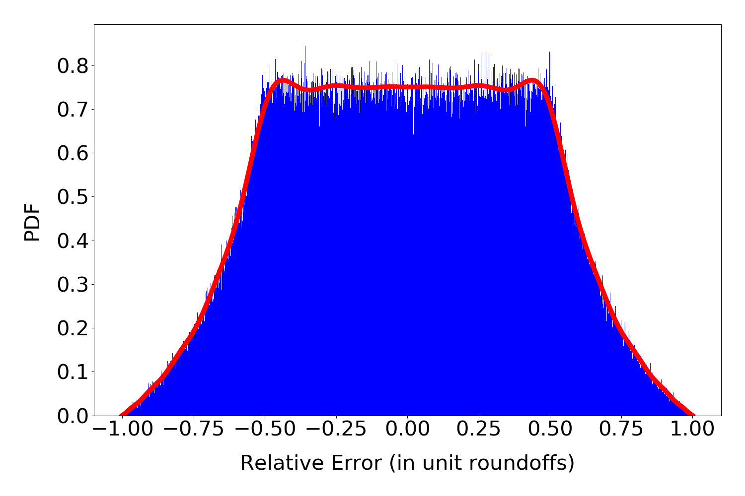
fig. 3 shows a plot of the half-precision error distribution for a random variable distributed uniformly on $\left[0,1\right]$. The red line is the density represented as a Chebyshev interpolating polynomial, the blue area is a histogram of the relative rounding error on one million samples. Note again the similarity with the typical density function represented in fig. 2.

With a concrete representation of the error distribution associated with an input distribution we can recursively evaluate the probabilistic interpretation of terms following (17). This computes the final output distribution (including probabilistic rounding errors) of a term, given input distributions for each of its variables. A simple application of this output distribution is range analysis.

We first consider a simple application of range analysis, namely the detection of overflows. To illustrate our probabilistic approach consider two variables $\tt x0,x1$ with $\tt x0$ distributed uniformly on $\left[10,15.5\right]$ and $\tt x1$ distributed uniformly on $\left[0.97,2\right]$. Suppose that the working precision is 3 bits for the exponent and 3 bits for the mantissa and that we are interested in the term $\tt x0/x1$. In infinite precision $15.5/0.97<16$, the largest representable number at the given precision level, and there is no overflow. In reduced precision however overflow can occur. In this case, an analyser like FPTaylor will correctly detect the overflow and return an infinite range, but will not be able to quantify the likelihood of overflow. fig. 4 shows the output distribution of the term $\tt x0/x1$ (red line), the support of the output distribution (‘PM’ in the legend), the output range of FPTaylor (‘FPT’ in the legend), and a histogram of the computation $\tt x0/x1$ performed on one million samples in reduced precision. Analytically, the probability of overflow is 0.0775%, and empirically 0.0642% of the samples overflow.

Next, we consider two benchmarks from FPBench [3] which our current setup can handle. In both cases we take half-precision as the working precision. The first benchmark is test02_sum8less which is given by the term:

with each $\tt xi$ assumed to be uniformly distributed on the interval $\left[1,2\right]$. The result of the range analysis are shown in fig. 5. The support of the output distribution provides marginally worse error bounds than FPTaylor and is in good agreement with one million Monte-Carlo simulations, that is to say one million evaluations of the term test02_sum8less in reduced precision where is input value is sampled uniformly from $\left[1,2\right]$. Crucially, we can probabilistically tighten these bound: at 99.99% confidence we can say that the output range lies in the interval $\left[9.0,15.0\right]$.

The second benchmark provides an even stronger case for considering probabilistic range analysis. Consider the multiplicative cousin of test02_sum8less given by the term test02_mul8less:

with each $\tt xi$ assumed to be uniformly distributed on the interval $\left[-3,3\right]$. The range analysis test02_mul8less is displayed in fig. 6. Again the support of the output distribution is marginally wider that the one provided by FPTaylor, but with 99.99% confidence we can tighten the output range by about five orders of magnitude in base 2 to $\left[-206,206\right]$.

References

- [1] Zachary Battles and Lloyd N Trefethen. An extension of matlab to continuous functions and operators. SIAM Journal on Scientific Computing, 25(5):1743–1770, 2004.
- [2] George A Constantinides, Peter YK Cheung, and Wayne Luk. Synthesis and optimization of DSP algorithms. Springer Verlag, 2004.
- [3] Nasrine Damouche, Matthieu Martel, Pavel Panchekha, Chen Qiu, Alexander Sanchez-Stern, and Zachary Tatlock. Toward a standard benchmark format and suite for floating-point analysis. In International Workshop on Numerical Software Verification, pages 63–77. Springer, 2016.
- [4] Eva Darulova, Anastasiia Izycheva, Fariha Nasir, Fabian Ritter, Heiko Becker, and Robert Bastian. Daisy-framework for analysis and optimization of numerical programs (tool paper). In International Conference on Tools and Algorithms for the Construction and Analysis of Systems, pages 270–287. Springer, 2018.
- [5] Nicholas J Higham. Accuracy and stability of numerical algorithms, volume 80. Siam, 2002.
- [6] Nicholas J Higham and Theo Mary. A new approach to probabilistic rounding error analysis. SIAM Journal on Scientific Computing, 41(5):A2815–A2835, 2019.
- [7] Ilse CF Ipsen and Hua Zhou. Probabilistic error analysis for inner products. arXiv preprint arXiv:1906.10465, 2019.
- [8] Szymon Jaroszewicz and Marcin Korzeń. Arithmetic operations on independent random variables: A numerical approach. SIAM Journal on Scientific Computing, 34(3):A1241–A1265, 2012.
- [9] Marcin Korzen and Szymon Jaroszewicz. PaCAL: A python package for arithmetic computations with random variables. Journal of Statistical Software, 57(10):5, 2014.
- [10] Dexter Kozen. Semantics of probabilistic programs. J. Comput. Syst. Sci., 22(3):328–350, June 1981.
- [11] Debasmita Lohar, Milos Prokop, and Eva Darulova. Sound probabilistic numerical error analysis. In International Conference on Integrated Formal Methods, pages 322–340. Springer, 2019.
- [12] Victor Magron, George Constantinides, and Alastair Donaldson. Certified roundoff error bounds using semidefinite programming. ACM Transactions on Mathematical Software (TOMS), 43(4):34, 2017.
- [13] Microprocessor Standards Committee of the IEEE Computer Society. IEEE Standard for Floating-Point Arithmetic, June 2019.
- [14] Douglass Stott Parker. Monte Carlo Arithmetic: exploiting randomness in floating-point arithmetic. University of California (Los Angeles). Computer Science Department, 1997.
- [15] Alexey Solovyev, Marek S Baranowski, Ian Briggs, Charles Jacobsen, Zvonimir Rakamarić, and Ganesh Gopalakrishnan. Rigorous estimation of floating-point round-off errors with symbolic taylor expansions. ACM Transactions on Programming Languages and Systems (TOPLAS), 41(1):20, 2018.
- [16] M.D. Springer. The algebra of random variables. Probability and Statistics Series. Wiley, 1979.
- [17] John Von Neumann and Herman H Goldstine. Numerical inverting of matrices of high order. Bulletin of the American Mathematical Society, 53(11):1021–1099, 1947.
Derivation of the typical distribution
We start by examining the quantity
which appears in eq. 7. Given a , we determine which floating point numbers make . We will write floating point numbers in the form
where , ranges from to and ranges from 0 to (and represents the mantissa). We can explicitly compute and . When we have:
and
For note simply that