Capacity of the covariance perceptron

Moritz Helias* Affiliation: Department of Physics, Faculty 1, RWTH Aachen University, Aachen, Germany

Abstract

The classical perceptron is a simple neural network that performs a binary classification by a linear mapping between static inputs and outputs and application of a threshold. For small inputs, neural networks in a stationary state also perform an effectively linear input-output transformation, but of an entire time series. Choosing the temporal mean of the time series as the feature for classification, the linear transformation of the network with subsequent thresholding is equivalent to the classical perceptron. Here we show that choosing covariances of time series as the feature for classification maps the neural network to what we call a ’covariance perceptron’; a mapping between covariances that is bilinear in terms of weights. By extending Gardner’s theory of connections to this bilinear problem, using a replica symmetric mean-field theory, we compute the pattern and information capacities of the covariance perceptron in the infinite-size limit. Closed-form expressions reveal superior pattern capacity in the binary classification task compared to the classical perceptron in the case of a high-dimensional input and low-dimensional output. For less convergent networks, the mean perceptron classifies a larger number of stimuli. However, since covariances span a much larger input and output space than means, the amount of stored information in the covariance perceptron exceeds the classical counterpart. For strongly convergent connectivity it is superior by a factor equal to the number of input neurons. Theoretical calculations are validated numerically for finite size systems using a gradient-based optimization of a soft-margin, as well as numerical solvers for the NP hard quadratically constrained quadratic programming problem, to which training can be mapped.

1 Introduction

Binary classification is one of the standard tasks in machine learning. The simplest artificial neural network that implements classification is the classical perceptron [1, 2, 3]. It is a feed-forward mapping from neurons in an input layer to those of an output layer. Neurons in the output layer receive a weighted sum of signals from the input layer, which is passed through a Heaviside nonlinearity, implementing a decision threshold. Inputs to the perceptron, i.e. activation levels of the input neurons, are specific features of some data, in the simplest case the pixels of an image or the time points of a temporal signal. Classification is achieved by training the weights from the input to the output layer such that the projections of different input patterns become linearly separable.

Classification is also one essential task for biological neuronal networks in the brain. However, neurons do not receive different static features of some input signal, but sequences of action potentials, so-called spikes, from other neurons. Biological neural networks thus have to extract the relevant features from these temporal sequences.

To understand biological information processing we need to ask which features of the temporal sequences contain the relevant information. Already in the 1950s it has been shown that the firing rate, i.e. the mean number of spikes in a given time interval, contains information for example on the presence of a certain feature of a stimulus, such as the orientation of a bar [4]. However, cortex also shows large temporal variability in responses even to the same stimuli [5] which raises the question whether this variability has some functional meaning. Evidence has accumulated that the temporal fluctuations of neuronal signals around their mean contain behaviorally relevant information; this holds even to the level of the exact timing of spikes [6]. For example, correlations in spike times across different neurons, such as precise synchronization, have been shown to code expectations of the animals [7].

Like in artificial neural networks, one mechanism for learning in the brain is implemented by changing the strengths of connections between neurons, known as synaptic plasticity. In the middle of the last century, Donald Hebb postulated the principle ’Cells that fire together, wire together’ [8, 9], a plasticity rule that depends on the activity of the connected neurons. Importantly, in Hebbian plasticity it is not the overall level of activation of the neurons (their overall firing rate) that is relevant, but the temporal coordination of activities. Since then, several learning rules were proposed to extract information from coordinated fluctuations [10, 11]. The model called spike-timing-dependent plasticity (STDP) [12] predicted that changes in synaptic strengths are sensitive to even the exact spike timings of the pre- and postsynaptic cells, which was confirmed later on in experiments [13, 14]. This suggests that temporal fluctuations in neural activities and their coordination are naturally distinguished features that shape learning and thereby the function of the neural circuit.

The simplest measure for coordination between temporal fluctuations are pairwise covariances between neural activities. In a network of $m$ neurons, pairwise cross-covariances form an $m(m-1)/2$ -dimensional space for coding information, which is a much larger space than the space of mean activities. This intuitively suggests that it might be beneficial for a neural system to make use of the covariances to represent and process relevant information. In this study, using methods from statistical mechanics, we examine the performance of such a computational paradigm which processes information that is represented in fluctuations: the covariance perceptron [15].

Neurons are highly nonlinear processing units. Nevertheless, in large networks where individual inputs to the neurons are small with respect to their total input, temporal fluctuations around some stationary state can be well explained by means of linear response theory [16]. In this setting, the network effectively performs a linear transformation between its inputs and outputs. Linear response theory has been shown to faithfully capture the statistics of fluctuations in asynchronous, irregular network states that are observed in cortex [17, 18].

In this study, we make use of linear response theory to show that a network that transforms temporal input signals into temporal output signals acts as a classical perceptron if the temporal mean of the network output trajectories is chosen as the relevant feature for a following binary classification. Choosing, instead, covariances as the relevant feature of the temporal signals, the same network acts as a covariance perceptron [15], which is based on a bilinear mapping in terms of weights, but linear from input to output covariances. The classical perceptron has been studied in the 1980s in terms of its performance for classification [19]. Two performance measures are the pattern capacity, the number of patterns that can be correctly classified into two distinct classes, and the information capacity, which is the number of bits a conventional computer requires to realize the same functionality as the neuronal implementation.

Here we set out to study the performance of the covariance-based classification paradigm by calculating the pattern capacity and information capacity of the covariance perceptron. Following Gardner’s theory of connections, we use replica symmetric mean-field theory with a saddle-point approximation to study the volume of possible weight configurations for the classification problem. The limiting capacity is given by the maximum number of correctly classifiable stimuli. This analysis shows that the covariance perceptron can store up to twice as many patterns as the classical perceptron. Moreover, in case of strongly convergent connectivity, the information capacity in bits largely exceeds the traditional paradigm by up to a factor $2m$ , with $m$ the number of input neurons. Our work thus provides evidence that covariance-based information processing in a biological context can reach superior performance compared to paradigms that have so far been used in artificial neuronal networks.

2 Model

Refer to caption — Figure 1: Setup. Top: Biological information processing. Sensory information enters the system as a time series. The dynamics of the neuronal network produces an outgoing time series of activities. Ultimately, a set of effectors, for example muscles, are controlled by the resulting signal. Bottom: Machine-learning view of the biological system. A set of features $F$ is extracted from the incoming time series. These are transformed by a mapping to another set of features $G$ , each of which is thresholded to produce a binary output, in the example encoding the movement direction. The input-output mapping is defined implicitly by the biological system.

In this study, we consider neural networks that transform patterns $x(t)$ of $m$ input trajectories $x_{k}(t)$ into patterns $y(t)$ of $n$ output trajectories $y_{i}(t)$ (Figure 1). Using this network transformation and a following hard decision threshold on the outputs, we want to perform a binary classification of patterns $x(t)$ into classes labeled by binary words $\zeta$ which entries can take the values $+1$ and $-1$ . Patterns $x(t)$ shall be defined by an $M$ -dimensional feature $F\in\mathbb{R}^{M}$ , and classification shall be performed on an $N$ -dimensional feature $G\in\mathbb{R}^{N}$ of the output patterns $y(t)$ . Possible features could, for example, be the signals at a given time point, their temporal average or some higher order statistics. By transforming patterns $x(t)$ into patterns $y(t)$ , the network maps the feature $F$ of the inputs to the feature $G$ of the outputs. The connection weights of the network thereby shall be trained to optimize the classification based on $G$ . In general, features $F$ and $G$ can describe very different characteristics of the patterns $x(t)$ and $y(t)$ , respectively. However, in this study we choose the case where $F$ and $G$ are of the same type, which is important for the consideration of multilayer networks.

An important measure for the quality of the classification is the margin defined as

\kappa=\min_{1\leq s\leq N}\min_{1\leq r\leq p}\left(\zeta_{s}^{r}G_{s}^{r}\right)\ ,

(1)

where $r$ indexes the patterns and $s$ the dimensions of the feature $G$ . The margin measures the smallest distance over all elements of $G$ from the threshold, here set to $0$ . It plays an important role for the robustness of the classification [20], as a larger margin tolerates more noise in the input pattern before classification is compromised. The margin of the classification is illustrated in Fig. 2, where each symbol represents one of the $p$ patterns and the colors and markers indicate the corresponding category $\zeta^{r}$ . Classification is achieved by training the connection weights of the network to maximize $\kappa$ . This optimization increases the gap and thus the separability between red and blue symbols and the disks and squares in Fig. 2.

The classification scheme reaches its limit for a certain pattern load $p$ at which the margin $\kappa$ vanishes. More generally, one can ask how many patterns the scheme can discriminate while maintaining a given minimal margin $\kappa$ . This defines the pattern capacity

\mathcal{P}(\kappa)=\max(p|\kappa).

(2)

The information capacity is the number of bits required in a conventional computer, if it were to realize the same classification of the $\mathcal{P}(\kappa)$ patterns

\mathcal{I}(\kappa)=\mathcal{P}(\kappa)\left(\log_{2}K+\log_{2}L\right).

(3)

Here $K$ denotes the number of possible configurations of a single pattern in the input, and $L$ denotes the number of possible binary words assigned to the output.

For any general network, one can write the output $y(t)$ as a Volterra series of the input $x(t)$ . Ongoing activity in cortical networks in many cases shows weakly-fluctuating activity with low correlations. It has been shown that such small fluctuations around some stationary state can be well described using linear response theory [16, 21, 22, 17], which amounts to a truncation of the Volterra series after the first order. In such a scenario, the network transformation of small inputs follows the general form

y(t)=\int dt^{\prime}W(t-t^{\prime})x(t^{\prime}),

(4)

with some generic linear response kernel $W(t)\in\mathbb{R}^{n\times m}$ . In the following, we will restrict our analysis to this scenario and study the computational properties of networks operating in the linear regime.

After having clarified the setup, let us now turn to two specific examples of features for classification.

Scenario 1: Classical perceptron

Let’s assume that the relevant feature of input trajectories $x_{k}(t)$ is their temporal mean which we here define as $X_{k}=\int dt\,x_{k}(t)$ (Fig. 3a)¹¹ 1 Note that, throughout, we consider observation times $T$ much larger than the decay time of the linear response kernels $W(t)$ . For brevity, we also drop the trivial normalization by the duration $T$ .. In this case, by integrating Eq. (4) over time, we see that the network performs the mapping

Y=WX

(5)

with weights $W_{ik}$ that are given by the area under the linear response kernels $W_{ik}=\int dt\,W_{ik}(t).$ The dimension of the input feature $F$ and output feature $G$ is then $M=m$ and $N=n$ , respectively.

Together with the application of a hard decision threshold on $Y$ , this network transformation acts as $n$ classical perceptrons. The weights $W_{ik}$ can be trained to reach optimal classification performance. The pattern capacity of a single classical perceptron classifying binary patterns has been shown to be [19, 9]

\displaystyle\mathcal{P}^{\mathrm{class}}(\kappa)

\displaystyle=

\displaystyle m\left(\int_{-\kappa}^{\infty}\frac{dt}{\sqrt{2\pi}}e^{-t^{2}/2}\left(t+\kappa\right)^{2}\right)^{-1}.

(6)

Note that this capacity does not increase by having more than $n=1$ outputs: all perceptrons receive the same patterns as inputs and therefore perform the same task. The information capacity for a classification scheme based on temporal means follows from Eqs. (2) and (3) with $K=2^{m}$ and $L=2^{n}$ as

\displaystyle\mathcal{I^{\mathrm{class}}}(\kappa)

\displaystyle=

\displaystyle\mathcal{P}^{\mathrm{class}}(\kappa)(m+n).

(7)

Note that in practical applications, one cannot observe input and output trajectories for infinite time, but only for a finite duration $T$ . The estimate of the mean activity from that finite period $T$ differs from the true temporal mean. Therefore, temporal fluctuations in the input trajectories constitute a source of noise in this classification paradigm.

Scenario 2: Covariance perceptron

We now turn to the contrary case where temporal fluctuations, quantified by the cross-covariances $P_{ij}(\tau)$ of the input trajectories, shall be the relevant feature for classification (Fig. 3b). In this case, the feature dimensions are $M=m(m-1)/2$ and $N=n(n-1)/2$ . The mapping from input covariances $P_{ij}(\tau)$ to output covariances $Q_{ij}(\tau)$ can be derived from Eq. (4) as

	$\displaystyle Q(\tau)$	$\displaystyle=$	$\displaystyle\int dt\,y(t)y^{\mathrm{T}}(t+\tau)-\int dt\,y(t)\int dty^{\mathrm{T}}(t+\tau)$
		$\displaystyle=$	$\displaystyle\int ds\int ds^{\prime}\,W(s)P(\tau+s-s^{\prime})W^{\mathrm{T}}(s^{\prime}).$

The network linearly filters the input covariances $P_{ij}(\tau)$ . If we consider covariances $Q_{ij}=\int d\tau\,Q_{ij}(\tau)$ integrated across all time lags, we obtain the simple mapping

Q=WPW^{\mathrm{T}},

(8)

which is linear in covariances but bilinear in the weights. Note that alternatively one could consider a single frequency component $\hat{Q}_{ij}=\int d\tau\,Q_{ij}(\tau)e^{-i\omega\tau}$ and derive an analogous mapping $\hat{Q}=\hat{W}\hat{P}\hat{W}^{\dagger}.$

Therefore, covariance-based classification amounts to a bilinear problem unlike the classical perceptron, which involves a linear mapping in terms of weights. In the following, we want to study the capacity of the covariance perceptron. But before we do so, it is important to note that the here considered network only acts as if it were a classical or covariance perceptron. The biological network itself in both cases receives the full input trajectories and creates the full output trajectories. However, the mapping between trajectories can either be optimized for a following classification of the temporal mean of the output trajectories (classical perceptron) or a classification based on the covariances of the output trajectories (covariance perceptron). In this way, the setup here is clearly different from standard machine learning approaches where one applies a feature selection on the inputs as a preprocessing step and only classifies this feature vector by a perceptron. The latter approach amounts to a linear mapping from $F$ to $G$ rather than a mapping between the entire trajectories (Figure 1).

3 Theoretical predictions for classification performance based on output cross-covariances

We now derive a theory for the pattern and information capacity of the covariance perceptron that is exact in the limit of large networks $m\to\infty$ and that can be compared to the seminal theory by Gardner [19] on the capacity of the classical perceptron. Formalizing the classification problem for a load of $p$ patterns, for each element $Q_{ij}^{r}$ of the readout matrix we draw a random label $\zeta_{ij}^{r}\in\{-1,1\}$ independently for each input pattern $P^{r}$ with $1\leq r\leq p$ . The task of the perceptron is to find a suitable weight matrix $W$ that leads to correct classification for all $p$ patterns. This requirement reads, for a given margin $\kappa>0$ ,

\zeta_{ij}^{r}Q_{ij}^{r}=\zeta_{ij}^{r}\;\big(WP^{r}W^{\mathrm{T}}\big)_{ij}>\kappa\ ,\quad\forall\ 1\leq r\leq p\ ,1\leq i<j\leq n.

(9)

We assume the patterns $P^{r}$ to be drawn randomly. This random ensemble allows us to employ methods from disordered systems [23]. Closely following the computation for the classical perceptron by Gardner [19, 9], the idea is to consider the replication of several covariance perceptrons. The replica, indexed by $\alpha$ and $\beta$ , have the same task defined by Eq. (9). The sets of patterns $P^{r}$ and labels $\zeta^{r}$ are hence the same for all replica, but each replicon has its own readout matrix $W^{\alpha}$ . If the task is not too hard, meaning that the pattern load $p$ is small compared to the number of free parameters $W_{ik}^{\alpha}$ , there are many solutions to Eq. (9). One thus considers the ensemble of all solutions and computes the typical overlap $R_{ij}^{\alpha\beta}\equiv\sum_{k=1}^{m}W_{ik}^{\alpha}W_{jk}^{\beta}$ between the solution $W^{\alpha}$ and $W^{\beta}$ in two different replica. The overlap is the scalar product of the weight vectors of outputs $i$ and $j$ . At a certain load $p=\mathcal{P}(\kappa)$ , up to the intrinsic reflection symmetry $W\mapsto-W$ in Eq. (9), there should only be a single solution left —the overlap $R_{ii}^{\alpha\beta}$ between solutions for identical readouts $i=j$ , but in different replica $\alpha\neq\beta$ , becomes unity. This pattern load defines the limiting capacity $\mathcal{P}$ .

Technically, the computation proceeds by defining the volume of all solutions for the whole set of cross-covariances $Q_{ij}^{r}$ that fulfill the classification task

\mathcal{V}=\int\mathrm{d}W\,\prod_{r}^{p}\prod_{i<j}^{n}\theta\Big(\zeta_{ij}^{r}\;\big(W\,P^{r}\,W^{\mathrm{T}}\big)_{ij}-\kappa\Big)\ .

(10)

Here $\theta$ denotes the Heaviside function and $\int dW=\prod_{i}^{n}\prod_{k}^{m}\int dW_{ik}$ . This equation is the analogue to Gardner’s approach of the perceptron; see [9, Section 10.2, eq. 10.83]. The typical behavior of the system for large $m$ is obtained by first taking the average of $\ln(\mathcal{V})$ over the ensemble of the patterns and labels. The assumption is that the system is self-averaging; for large $m$ the capacity should not depend much on the particular realization of patterns. The average of $\ln(\mathcal{V})$ can be computed by the replica trick $\langle\ln(\mathcal{V})\rangle=\lim_{q\to 0}\,\big(\langle\mathcal{V}^{q}\rangle-1\big)/q$ [23] which amounts to considering $q$ systems that have identical realizations of patterns.

3.0.1 Patterns and classification labels

In order to perform the average over the patterns and labels, we need to specify their statistics. Here, we choose a symmetric setting with independent and identically distributed labels $\zeta_{i<j}^{r}=\pm 1$ , each with probability $1/2$ . In contrast to inputs to the classical perceptron which can be chosen independently, covariances involve constraints related to the fact that a covariance matrix is positive semidefinite, which implies in particular

$\displaystyle P_{kl}$	$\displaystyle=$	$\displaystyle P_{lk}\ ,$	(11)
$\displaystyle P_{kk}$	$\displaystyle\geq$	$\displaystyle 0\ ,$
$\displaystyle\|P_{kl}\|$	$\displaystyle\leq$	$\displaystyle\sqrt{P_{kk}\,P_{ll}}\ ,$

for all indices $k$ and $l$ . A simple way to ensure positive semidefiniteness is to choose each input covariance pattern to be of the form

P^{r}=1_{m}+\chi^{r}\ ,

(12)

with $1_{m}$ being the $m\times m$ identity matrix and a symmetric random matrix $\chi^{r}=\left(\chi^{r}\right)^{\mathrm{T}}$ with vanishing diagonal entries $\chi_{kk}^{r}=0$ and independent and identically distributed lower off-diagonal elements $\chi_{k<l}^{r}=\pm c$ , each with probability $f/2$ , and $\chi_{k<l}^{r}=0$ with probability $1-f$ .

Here $f$ controls the sparseness (or density) of the non-zero cross-covariances. The constraint of $P_{kk}=1$ firstly enforces that all information of the patterns is in the off-diagonal elements. Secondly, it ensures the positive semidefiniteness for a sufficiently broad range of values for $c$ and $f$ .

The specific form of the input covariances (12) implies with Eq. (8) that

Q_{ii}^{r}=\sum_{k}^{m}(W_{ik})^{2}+\sum_{k\neq l}^{m}W_{ik}W_{il}\chi_{kl}^{r}\qquad\forall\,i,r\ ,

which, on expectation over patterns, yields

\langle Q_{ii}^{r}\rangle_{\chi}=\sum_{k}^{m}(W_{ik})^{2}\mathrel{{\mathop{=}\limits}}1\qquad\forall\,i\ .

(13)

The magnitude of output variances is therefore given by the normalization of the row vectors of $W$ , which we here set to unity. This ensures that we have a self-consistent scheme, where information in the input and the output is both encoded only in cross-covariances. Note that this self-consistency is only reached on expectation as each entry $Q_{ii}^{r}$ varies around $1$ according to the magnitude of cross-covariances $\chi$ , which, however, for large networks is much smaller than the variance [24, 25, 26]. Forcing $Q_{ii}^{r}=1$ would unnecessarily complicate the analysis; simulation results below show equal capacity with or without this hard constraint. Finally, note that the value of unity for the variance does not restrict the generality of this analysis as any other value of the variance will lead to another normalization of the weights $W$ , which can be absorbed in the margin $\kappa$ (cf. Eq. (9)).

3.0.2 Pattern and label average

Given the constraint on the length of the rows in the weight matrix $W$ , Eq. (13), we obtain for the expectation of the power of the volume in Eq. (10)

	$\displaystyle\langle\mathcal{V}^{q}\rangle$	$\displaystyle=$	$\displaystyle\left\langle\prod_{\alpha}^{q}\int dW^{\alpha}\,\prod_{i}^{n}\delta\Big(\sum_{k}^{m}(W_{ik}^{\alpha})^{2}-1\Big)\,\prod_{r}^{p}\,\prod_{i<j}^{n}\,\theta\Big(\tilde{Q}_{ij}^{r\alpha}-\kappa\Big)\right\rangle_{\zeta,\chi}$		(14)
	$\displaystyle\tilde{Q}_{ij}^{r\alpha}$	$\displaystyle=$	$\displaystyle\zeta_{ij}^{r}(W^{\alpha}P^{r}W^{\alpha\mathrm{T}})_{ij}\ ,$

which we need to study in the limit $q\rightarrow 0$ . Note the Dirac delta distribution $\delta$ that describes the constraint (13) on the length of the weight vectors. The pattern average amounts to averaging

$\displaystyle\left\langle\prod_{\alpha}^{q}\prod_{r}^{p}\prod_{i<j}^{n}\theta\Big(\tilde{Q}_{ij}^{r\alpha}-\kappa\Big)\right\rangle_{\zeta,\chi}$	$\displaystyle=$	$\displaystyle\prod_{r}^{p}\left\langle\prod_{\alpha}^{q}\prod_{i<j}^{n}\theta\Big(\tilde{Q}_{ij}^{r\alpha}-\kappa\Big)\right\rangle_{\zeta,\chi}$	(15)
	$\displaystyle=$	$\displaystyle\left\langle\prod_{\alpha}^{q}\prod_{i<j}^{n}\theta\Big(\tilde{Q}_{ij}^{r\alpha}-\kappa\Big)\right\rangle_{\zeta,\chi}^{p}$
	$\displaystyle\equiv$	$\displaystyle\mathcal{G}^{p}\,,$

where we used that patterns and labels are uncorrelated (first line) and follow the same statistics (second line). We can express $\mathcal{G}$ in terms of cumulants of $\tilde{Q}_{ij}^{r\alpha}$ by rewriting the Heaviside function

	$\displaystyle\theta\Big(\tilde{Q}_{ij}^{r\alpha}-\kappa\Big)$	$\displaystyle=$	$\displaystyle\int_{\kappa}^{\infty}dx_{ij}^{\alpha}\,\delta\big(\tilde{Q}_{ij}^{r\alpha}-x_{ij}^{\alpha}\big)$		(16)
		$\displaystyle=$	$\displaystyle\int_{\kappa}^{\infty}\mathrm{d}x_{ij}^{\alpha}\int_{-i\infty}^{i\infty}\frac{\mathrm{d}\tilde{x}_{ij}^{\alpha}}{2\pi i}\,e^{\tilde{x}_{ij}^{\alpha}\big(\tilde{Q}_{ij}^{r\alpha}-x_{ij}^{\alpha}\big)},$		(16)

such that

$\displaystyle\mathcal{G}$	$\displaystyle=$	$\displaystyle\prod_{i<j}^{n}\left\{\int Dx_{ij}\int D\tilde{x}_{ij}\right\}\,e^{-\sum_{\alpha}^{q}\sum_{i<j}^{n}\tilde{x}_{ij}^{\alpha}x_{ij}^{\alpha}}\left\langle e^{\sum_{\alpha}^{q}\sum_{i<j}^{n}\tilde{x}_{ij}^{\alpha}\tilde{Q}_{ij}^{r\alpha}}\right\rangle_{\zeta,\chi}$	(17)
	$\displaystyle=$	$\displaystyle\prod_{i<j}^{n}\left\{\int Dx\int D\tilde{x}\,e^{-\sum_{\alpha}^{q}\tilde{x}^{\alpha}x^{\alpha}+\frac{1}{2}\sum_{\alpha,\beta}^{q}\,\tilde{x}^{\alpha}\left\langle\left\langle\tilde{Q}_{ij}^{r\alpha}\tilde{Q}_{ij}^{r\beta}\right\rangle\right\rangle_{\zeta,\chi}\tilde{x}^{\beta}}\right\}$
	$\displaystyle\equiv$	$\displaystyle\prod_{i<j}^{n}\mathcal{G}_{ij}\,.$

Here we used the abbreviations $\int Dx\equiv\prod_{\alpha}^{q}\int_{\kappa}^{\infty}\mathrm{d}x^{\alpha}$ and $\int D\tilde{x}\equiv\prod_{\alpha}^{q}\int_{-i\infty}^{i\infty}\frac{\mathrm{d}\tilde{x}^{\alpha}}{2\pi i}$ , where indices of integration variables in the second line have been dropped. We further identified the moment generating function of the variables $\tilde{Q}_{ij}^{r\alpha}$ with respect to the statistics of $\zeta$ and $\chi$ (first line). The latter can be expanded in cumulants (second line): In the large- $m$ limit, this expansion can be truncated at the second cumulant $\left\langle\left\langle\tilde{Q}_{ij}^{r\alpha}\tilde{Q}_{kl}^{r\beta}\right\rangle\right\rangle_{\zeta,\chi}$ in a similar fashion to the classical perceptron [9]. Due to the independence of labels $\zeta_{ij}$ and $\zeta_{kl}$ , the second cumulants vanish if $i\neq k$ or $j\neq l$ . The diagonal elements are given by

$\displaystyle\left\langle\left\langle\tilde{Q}_{ij}^{r\alpha}\tilde{Q}_{ij}^{r\beta}\right\rangle\right\rangle_{\zeta,\chi}$	$\displaystyle=$	$\displaystyle\Big(\sum_{k}^{m}W_{ik}^{\alpha}W_{jk}^{\alpha}\Big)\,\Big(\sum_{k}^{m}W_{ik}^{\beta}W_{jk}^{\beta}\Big)$	(18)
		$\displaystyle+fc^{2}\,\Big(\sum_{k}^{m}W_{ik}^{\alpha}W_{ik}^{\beta}\Big)\,\Big(\sum_{k}^{m}W_{jk}^{\alpha}W_{jk}^{\beta}\Big)$
		$\displaystyle+fc^{2}\,\Big(\sum_{k}^{m}W_{ik}^{\alpha}W_{jk}^{\beta}\Big)\,\Big(\sum_{k}^{m}W_{ik}^{\beta}W_{jk}^{\alpha}\Big)\ .$

The first term arises from the diagonal $1_{m}$ in the patterns $P^{r}$ in Eq. (12), and the third term stems from the symmetry of $P^{r}$ . These two terms would be absent for completely uncorrelated i.i.d. matrices $P^{r}$ . In the second and third lines in Eq. (18) we added a single term $k=l$ which is negligible in the large- $m$ limit. We see that the only dependence on the sparseness $f$ and the magnitude $c$ of input covariances is in the form $fc^{2}$ —it does not depend on these two parameters separately. The problem is, moreover, now symmetric in all $i<j$ index pairs. We also observe that the product over all $p$ patterns has identical factors that do not depend on the pattern index $r$ , so that we only get this factor to the $p$ -th power.

3.0.3 Auxiliary field formulation

Starting from Eq. (18), we now define the auxiliary fields as

R_{ij}^{\alpha\beta}\equiv\sum_{k}^{m}W_{ik}^{\alpha}W_{jk}^{\beta}\ ,

(19)

for $i<j$ and $\alpha\neq\beta$ . The field $R_{ij}^{\alpha\alpha}$ for $i\neq j$ measures the overlap between weight vectors to different units in the same replicon $\alpha$ . It contributes to the average value of $Q_{ij}^{r\alpha}$ because the unit diagonal (common to all $P^{r}$ ) is weighted by $R_{ij}^{\alpha\alpha}$ . Hence the output $Q_{ij}^{r\alpha}$ will be displaced by $R_{ij}^{\alpha\alpha}$ irrespective of the realization of $P^{r}$ . $R_{ij}^{\alpha\beta}$ for $\alpha\neq\beta$ measures the overlap of weight vectors in different replica. For $\alpha=\beta$ and $i=j$ we have $R_{ii}^{\alpha\alpha}=1$ due to Eq. (13). The definitions Eq. (19) are enforced by integrations over Dirac distributions

\displaystyle\delta\big(\sum_{k}^{m}W_{ik}^{\alpha}W_{jk}^{\beta}-R_{ij}^{\alpha\beta}\big)

\displaystyle=

\displaystyle\int_{-i\infty}^{i\infty}\frac{\mathrm{d}\tilde{R}_{ij}^{\alpha\beta}}{2\pi i}\,e^{-\tilde{R}_{ij}^{\alpha\beta}\sum_{k}^{m}W_{ik}^{\alpha}W_{jk}^{\beta}+\tilde{R}_{ij}^{\alpha\beta}R_{ij}^{\alpha\beta}}

(20)

Note that the same Fourier representation can also be used for the length constraint on the weight vectors $\delta\big((W^{\alpha}W^{\alpha\mathrm{T}})_{ii}-1\big)$ . After inserting auxiliary fields into Eq. (17), the integration over weights $W_{ik}^{\alpha}$ only applies to the first term in Eq. (20) for all indices

	$\displaystyle\prod_{\alpha}^{q}\prod_{i}^{n}\prod_{k}^{m}\int dW_{ik}^{\alpha}\,\exp\big(-\sum_{\alpha,\beta}^{q}\sum_{i\leq j}^{n}\tilde{R}_{ij}^{\alpha\beta}\sum_{k}^{m}W_{ik}^{\alpha}W_{jk}^{\beta}\big)$	(21)
$\displaystyle=$	$\displaystyle\left(\prod_{\alpha}^{q}\prod_{i}^{n}\int dW_{i}^{\alpha}\,\exp\big(-\sum_{\alpha,\beta}^{q}\sum_{i\leq j}^{n}\tilde{R}_{ij}^{\alpha\beta}W_{i}^{\alpha}W_{j}^{\beta}\big)\right)^{m}$
$\displaystyle\equiv$	$\displaystyle\mathcal{F}^{m}\,.$

Here, we used that the expression factorizes in the index $k$ so that we get the same integral to the $m$ -th power, one factor for each component $W_{ik}^{\alpha}\,\forall k=1,\ldots,m$ , allowing us to define a single integration variable $W_{i}^{\alpha}$ . Gathering contributions from the second term in Eq. (20) for all indices defines

\mathcal{H}\equiv\sum_{\alpha,\beta}^{q}\sum_{i\leq j}^{n}\tilde{R}_{ij}^{\alpha\beta}R_{ij}^{\alpha\beta}.

(22)

Expressing $\left\langle\mathcal{V}^{q}\right\rangle$ in terms of $\mathcal{F}$ , $\mathcal{G}_{ij}$ and $\mathcal{H}$ then yields

\displaystyle\left\langle\mathcal{V}^{q}\right\rangle

\displaystyle=

\displaystyle\int\mathrm{d}R\int\mathrm{d}\tilde{R}\,\exp\big(m\,\ln(\mathcal{F})+p\sum_{i<j}^{n}\ln(\mathcal{G}_{ij})+\mathcal{H}\big),

(23)

with $\int\mathrm{d}R\equiv\prod_{\alpha,\beta}^{q}\prod_{i<j}^{n}\int\mathrm{d}R_{ij}^{\alpha\beta}\prod_{\alpha\neq\beta}^{q}\int\mathrm{d}R_{ii}^{\alpha\beta}$ and $\int\mathrm{d}\tilde{R}=\prod_{\alpha,\beta}^{q}\prod_{i\leq j}^{n}\int_{-i\infty}^{i\infty}\frac{\mathrm{d}\tilde{R}_{ij}^{\alpha\beta}}{2\pi i}$ .

The leading order behavior for $m\to\infty$ follows as a mean-field approximation in the auxiliary variables $R_{ij}^{\alpha\beta}$ . Therefore, we are interested in the saddle points of the integrals $\int\mathrm{d}R\int\mathrm{d}\tilde{R}$ and search for a replica-symmetric solution. We therefore set

	$\displaystyle R_{ij}^{\alpha\alpha}=R_{ij}^{=},$	$\displaystyle\hskip 10.00002pt\tilde{R}_{ij}^{\alpha\alpha}=\tilde{R}_{ij}^{=}$			(24)
	$\displaystyle R_{ij}^{\alpha\beta}=R_{ij}^{\neq},$	$\displaystyle\hskip 10.00002pt\tilde{R}_{ij}^{\alpha\beta}=\tilde{R}_{ij}^{\neq}$

for $\alpha\neq\beta$ . For replica symmetry, the exponent in $\mathcal{G}_{ij}$ simplifies to

	$\displaystyle\sum_{\alpha,\beta}^{q}\,\tilde{x}^{\alpha}\Big(R_{ij}^{\alpha\alpha}R_{ij}^{\beta\beta}+fc^{2}\,R_{ii}^{\alpha\beta}\,R_{jj}^{\alpha\beta}+fc^{2}\,R_{ij}^{\alpha\beta}\,R_{ij}^{\beta\alpha}\Big)\tilde{x}^{\beta}$
	$\displaystyle=(\lambda_{ij}^{=}-\lambda_{ij}^{\neq})\sum_{\alpha}^{q}\,\tilde{x}^{\alpha}\tilde{x}^{\alpha}+\lambda_{ij}^{\neq}\left(\sum_{\alpha}^{q}\,\tilde{x}^{\alpha}\right)^{2}\ ,$		(25)

with $\lambda_{ij}^{=}=fc^{2}\,R_{ii}^{=}R_{jj}^{=}+(1+fc^{2})\,R_{ij}^{=2}$ and $\lambda_{ij}^{\neq}=fc^{2}\,R_{ii}^{\neq}R_{jj}^{\neq}+R_{ij}^{=2}+fc^{2}\,R_{ij}^{\neq 2}$ . The replica are coupled by the factor $\lambda_{ij}^{\neq}$ , which renders $\int\mathrm{D}\tilde{x}$ in $\mathcal{G}_{ij}$ a $q$ -dimensional integral. In order to apply the limit $q\rightarrow 0$ , it is convenient to decouple the replica by performing the Hubbard-Stratonovich transformation

e^{\frac{1}{2}\lambda_{ij}^{\neq}\Big(\sum_{\alpha}^{q}\,\tilde{x}^{\alpha}\Big)^{2}}=\int Dt\,e^{t\sqrt{\lambda_{ij}^{\neq}}\sum_{\alpha}^{q}\,\tilde{x}^{\alpha}}\ ,

(26)

with $\int Dt\equiv\int_{-\infty}^{\infty}\frac{dt}{\sqrt{2\pi}}e^{-t^{2}/2}$ , which turns the $2q$ -dimensional integral over $x^{\alpha}$ and $\tilde{x}^{\alpha}$ for $1\leq\alpha\leq q$ into a Gaussian integral over the $q$ -th power of a function $g_{ij}(t)$ that is given by a two-dimensional integral

	$\displaystyle g_{ij}(t)$	$\displaystyle=$	$\displaystyle\int_{\kappa}^{\infty}\mathrm{d}x\int_{-i\infty}^{i\infty}\frac{\mathrm{d}\tilde{x}}{2\pi i}\,e^{\frac{1}{2}(\lambda_{ij}^{=}-\lambda_{ij}^{\neq})\tilde{x}^{2}+t\sqrt{\lambda_{ij}^{\neq}}\tilde{x}-\tilde{x}x}$		(27)
		$\displaystyle=$	$\displaystyle\frac{1}{2}\mathrm{erfc}(a_{ij}(t))\ ,$		(27)

with $a_{ij}(t)=(\kappa-t\sqrt{\lambda_{ij}^{\neq}})/\sqrt{2(\lambda_{ij}^{=}-\lambda_{ij}^{\neq})}$ . The resulting form of $\mathcal{G}_{ij}$ allows us to take advantage of the $q\rightarrow 0$ limit by approximating

$\displaystyle\ln(\mathcal{G}_{ij})$	$\displaystyle=$	$\displaystyle\ln\left\langle g_{ij}(t)^{q}\right\rangle=\ln\left\langle\exp\left(q\ln\big(g_{ij}(t)\big)\right)\right\rangle$	(28)
	$\displaystyle\rightarrow$	$\displaystyle\ln\left(1+q\left\langle\ln\big(g_{ij}(t)\big)\right\rangle\right)\rightarrow q\left\langle\ln\big(g_{ij}(t)\big)\right\rangle$
	$\displaystyle=$	$\displaystyle q\left\langle\ln\Big(\mathrm{erfc}\big(a_{ij}(t)\big)\Big)\right\rangle+\ln(1/2)\ .$

3.0.4 Replica limit $q\rightarrow 0$

So far, we considered $q$ replica of the system, where $q$ was a natural number. In order to find the typical behavior of $\mathcal{V}$ , the replica trick requires us to study the limit $q\rightarrow 0$ . Using $q(q-1)=-q+\mathcal{O}(q^{2})$ , we get

\mathcal{H}=q\sum_{i\leq j}^{n}\tilde{R}_{ij}^{=}R_{ij}^{=}-q\sum_{i\leq j}^{n}\tilde{R}_{ij}^{\neq}R_{ij}^{\neq},

(29)

which gives rise to the following saddle point equations

	$\displaystyle R_{ij}^{=}$	$\displaystyle=$	$\displaystyle-\frac{m}{q}\frac{\partial\ln(\mathcal{F})}{\partial\tilde{R}_{ij}^{=}}\ ,\hskip 10.00002ptR_{ij}^{\neq}=\frac{m}{q}\frac{\partial\ln(\mathcal{F})}{\partial\tilde{R}_{ij}^{\neq}}$		(30)
	$\displaystyle\tilde{R}_{ij}^{=}$	$\displaystyle=$	$\displaystyle-\frac{p}{q}\sum_{k<l}^{n}\frac{\partial\ln(\mathcal{G}_{kl})}{\partial R_{ij}^{=}}\ ,\hskip 10.00002pt\tilde{R}_{ij}^{\neq}=\frac{p}{q}\sum_{k<l}^{n}\frac{\partial\ln(\mathcal{G}_{kl})}{\partial R_{ij}^{\neq}}.$		(31)

The above equations show that we need to find the contribution of $\ln(\mathcal{F})$ and $\ln(\mathcal{G}_{ij})$ proportional to $q$ as this is the only term surviving in the $q\rightarrow 0$ limit.

3.0.5 Limiting pattern load $p\rightarrow\mathcal{P}(\kappa)$

We are interested in the limit $p\rightarrow\mathcal{P}(\kappa)$ , which denotes the point where only a single solution is found: the overlap $R_{ii}^{\neq}\to R_{ii}^{=}=1$ of the readout between replica is identical to the length of the vector in each individual replicon, so only a single solution is found. So we set $R_{ii}^{\neq}=1-\epsilon$ and study the limit $\epsilon\rightarrow 0$ for all $i\in[1,m]$ simultaneously. We need to be careful in taking this limit as $\ln(\mathcal{G}_{ij})$ is singular for $\epsilon=0$ . The saddle-point equations relate derivatives of $\ln(\mathcal{G}_{ij})$ to tilde-fields, which in turn are defined by $\ln(\mathcal{F})$ . A singularity in $\ln(\mathcal{G}_{ij})$ at $\epsilon=0$ therefore implies also a singularity in $\ln(\mathcal{F})$ . These singularities will cancel in the following calculation of the capacity.

We first focus on the fields $R_{ij}^{=}$ and $R_{ij}^{\neq}$ for $i<j$ : The function $\ln G_{ij}$ depends quadratically on $R_{ij}^{=}$ and $R_{ij}^{\neq}$ (see Eq. (25)). The same is true for $\mathcal{F}$ , which can be seen by Taylor expansion around $\tilde{R}_{ij}^{=}=\tilde{R}_{ij}^{\neq}=0$ (cp. Eq. (21)): all odd Taylor coefficients vanish since they are determined by odd moments of a Gaussian integral with zero mean. By rewriting Eq. (31) as $\tilde{R}_{ij}^{=}=-2R_{ij}^{=}\frac{p}{q}\sum_{k<l}^{n}\frac{\partial\ln(\mathcal{G}_{kl})}{\partial R_{ij}^{=2}}$ and $R_{ij}^{=}=-2\tilde{R}_{ij}^{=}\frac{m}{q}\frac{\partial\ln(\mathcal{F})}{\partial\tilde{R}_{ij}^{=2}}$ , respectively, and analogously for $\tilde{R}_{ij}^{\neq}$ and $R_{ij}^{\neq}$ , we see that $R_{ij}^{=}=\tilde{R}_{ij}^{=}=R_{ij}^{\neq}=\tilde{R}_{ij}^{\neq}=0$ is a solution to the saddle point equations. This solution makes sense as $R_{ij}^{=}$ represents a displacement of the $Q_{ij}$ irrespective of the label $\zeta^{r}=\pm 1$ . Thus the perceptron would lose flexibility in assigning arbitrary labels to patterns; a non-vanishing value would therefore hinder the classification. Figure 4 shows the numerically calculated overlap $R_{ij}^{=}$ to be close to zero, as predicted by the theory. At the point of limiting capacity all replica find the same solution. Therefore, also the overlap $R_{ij}^{\neq}$ across replica must vanish. Using $\tilde{R}_{ij}^{=}=\tilde{R}_{ij}^{\neq}=0$ , an analogous procedure as in Section 3.0.4 can be performed to calculate the term $\ln(\mathcal{F})$ in the $q\rightarrow 0$ limit

\ln(\mathcal{F})\rightarrow-\frac{1}{2}q\sum_{i}^{n}\left(\ln\left(\tilde{R}_{ii}^{=}-\tilde{R}_{ii}^{\neq}\right)+\tilde{R}_{ii}^{\neq}/\left(\tilde{R}_{ii}^{=}-\tilde{R}_{ii}^{\neq}\right)\right)+\mathrm{const}\ .

(32)

Then Eq. (30) can be easily solved to obtain

\tilde{R}_{ii}^{=}=-\frac{m}{2}\frac{1-2\epsilon}{\epsilon^{2}},\hskip 10.00002pt\tilde{R}_{ii}^{\neq}=-\frac{m}{2}\frac{1-\epsilon}{\epsilon^{2}}\ .

(33)

Inserting this solution into Eq. (31) and using Eq. (28), we get in the limit $\epsilon\rightarrow 0$

$\displaystyle-\frac{m}{2}\frac{1}{\epsilon^{2}}$	$\displaystyle=$	$\displaystyle\mathcal{P}(\kappa)\sum_{k<l}^{n}\left(\frac{\partial\left\langle\ln\Big(\mathrm{erfc}(a_{kl}(t))\Big)\right\rangle}{\partial R_{kk}^{\neq}}\delta_{ki}+(k\leftrightarrow l)\right)$
	$\displaystyle=$	$\displaystyle\mathcal{P}(\kappa)\sum_{k<l}^{n}\int Dt\frac{\frac{\partial}{\partial a_{kl}(t)}\mathrm{erfc}(a_{kl}(t))}{\mathrm{erfc}(a_{kl}(t))}\left(\frac{\partial a_{kl}(t)}{\partial R_{kk}^{\neq}}\delta_{ki}+\frac{\partial a_{kl}(t)}{\partial R_{ll}^{\neq}}\delta_{li}\right)$
	$\displaystyle=$	$\displaystyle\mathcal{P}(\kappa)\sum_{k<l}^{n}\int Dt\frac{-\frac{2}{\sqrt{\pi}}e^{-a_{kl}(t)^{2}}}{\mathrm{erfc}(a_{kl}(t))}\left(\frac{\partial a_{kl}(t)}{\partial R_{kk}^{\neq}}\delta_{ki}+\frac{\partial a_{kl}(t)}{\partial R_{ll}^{\neq}}\delta_{li}\right).$

For $\epsilon\rightarrow 0$ the function $a_{kl}(t)$ goes to negative infinity for $t>\kappa/\sqrt{fc^{2}}$ and $\mathrm{erfc}(a_{kl}(t))\rightarrow 2$ . In this case the numerator in the integrand makes the integral vanish. Therefore, we can restrict the integration range to $t\in(-\infty,\kappa/\sqrt{fc^{2}}]$ , where $a_{kl}(t)\rightarrow\infty$ for $\epsilon\rightarrow 0$ , such that we can insert the limit behavior of $\mathrm{erfc}(a_{kl}(t))\rightarrow e^{-a_{kl}(t)^{2}}/(\sqrt{\pi}a_{kl}(t))$ . Using

\frac{\partial a_{kl}(t)^{2}}{\partial R_{kk}^{\neq}}\rightarrow\frac{\left(\kappa-t\sqrt{fr^{2}}\right)^{2}}{2fr^{2}(1-(1-\epsilon)^{2})^{2}}+\mathcal{O}\left(\frac{1}{\epsilon}\right)\rightarrow\frac{\left(\bar{\kappa}-t\right)^{2}}{8\epsilon^{2}}+\mathcal{O}\left(\frac{1}{\epsilon}\right),

(34)

where we introduced $\bar{\kappa}=\kappa/\sqrt{fr^{2}}$ , the limiting number of patterns $\mathcal{P}(\kappa)$ follows from

\frac{m}{\epsilon^{2}}=\mathcal{P}(\kappa)\int_{-\infty}^{\bar{\kappa}}\frac{dt}{\sqrt{2\pi}}\exp\left(-\frac{t^{2}}{2}\right)\frac{\left(\bar{\kappa}-t\right)^{2}}{4\epsilon^{2}}\sum_{k<l}^{n}\left(\delta_{ki}+\delta_{li}\right)

\mathcal{P}(\kappa)=4\frac{m}{n-1}\left(\int_{-\bar{\kappa}}^{\infty}\frac{dt}{\sqrt{2\pi}}\exp\left(-\frac{t^{2}}{2}\right)\left(t+\bar{\kappa}\right)^{2}\right)^{-1}.

(35)

4 Results

In the following, we present the key conclusions from the theoretical derivation of Eq. (35) as well as numerical validations.

The pattern capacity grows linearly in the number of inputs.

Analogous to the classical perceptron, the pattern capacity is an extensive quantity in the number of inputs: $\mathcal{P\sim}m$ . This result is obvious as a higher-dimensional space facilitates classification. Formally, this is shown by the problem factorizing in the input indices in the saddle-point approximation.

The pattern capacity depends on the rescaled margin.

The pattern capacity only depends on the margin through the parameter $\bar{\kappa}\equiv\kappa/\sqrt{fc^{2}}$ , which measures the margin $\kappa$ relative to the standard deviation of the readout (Figure 5). This is also true for the classical perceptron, which was originally analyzed for $fc^{2}=1$ . In the latter case, the result is simple as, for random patterns $\xi$ with standard deviation $\sqrt{fc^{2}}$ , the inequality $\zeta_{i}\big(W\xi\big)_{i}>\kappa$ is equivalent to $\zeta_{i}\big(W\tilde{\xi}\big)_{i}>\kappa/\sqrt{fc^{2}}=\bar{\kappa}$ with rescaled patterns $\tilde{\xi}$ of unit standard deviation. In the case of the covariance perceptron, the situation is more subtle due to the identity matrix contained in the patterns $P=1+\chi$ . However, due to the orthogonality of the weight vectors $WW^{\mathrm{T}}=0$ (Figure 4) the same scaling arguments hold in Eq. (9). Note that the orthogonality arises naturally as a non-zero overlap $R_{ij}^{=}$ between different weight vectors ( $i\neq j$ ) would cause a bias in outputs and therefore hinder classification of $Q_{ij}$ around zero.

Similarly, the replica-symmetric solution is agnostic to the specificity in patterns $P$ with regard to symmetry of $\chi$ . This can be seen from the terms including $R_{ij}^{\neq}$ , which only arise due to the symmetry: the replica-symmetric solution of the saddle-point equations implies $R_{ij}^{\neq}=0$ , i.e. orthogonality of different weight vectors in different replica. Physically, it makes sense that at the limiting pattern load, all replica behave similarly.

In addition to the fact that for both perceptrons $\bar{\kappa}$ is the determining quantity, the dependence of the pattern capacity on $\bar{\kappa}$ is also identical. The derivation in Section 3 explains this structural similarity: The functions $\mathcal{F}$ and $\mathcal{H}$ are the same for both perceptrons as they follow from the length constraint on the weight vectors and the introduction of the auxiliary fields in Eq. (19). The latter are identical for both perceptrons. Also the structure of $\mathcal{G}$ and its dependence on $a(t)$ is the same in both cases, resulting in the integral in Eq. (35).

A single readout has a four times higher pattern capacity than the classical perceptron.

For a single readout ( $N=1\rightarrow n=2$ ), the pattern capacity of the covariance perceptron is four times larger than the pattern capacity of the classical perceptron (Figure 5b)

\displaystyle\mathcal{P}^{\mathrm{cov}}(\bar{\kappa})

\displaystyle=

\displaystyle 4\mathcal{P}^{\mathrm{class}}(\bar{\kappa}).

(36)

The superior pattern capacity of the covariance perceptron can be understood intuitively: For a single readout, the problem to be solved reads $Q_{12}=\check{W}^{1\mathrm{T}}\,P\,\check{W}^{2}$ , which is bilinear in $\check{W}^{1}$ and $\check{W}^{2}$ , the first and second row of the weight matrix $W$ . Choosing $\check{W}^{1}$ as a random vector can only lead to the same or worse classification performance than optimizing $\check{W}^{1}$ for the given set of patterns: the product $\check{W}^{1\mathrm{T}}\,P\equiv\xi$ can be considered a random pattern and optimizing only $\check{W}^{2}$ thus amounts to a classical perceptron. Therefore, optimizing both, $\check{W}^{1}$ and $\check{W}^{2}$ , the performance must be larger or equal to that of a linear perceptron. For $N\gg 1$ , different rows $\check{W}^{i}$ are not independent, as each row determines multiple output covariances $Q_{ij}$ . These amount to additional constraints in the optimization and thus a reduction in pattern capacity (see below).

Formally, the different scaling (factor $4$ in Eq. 35) of the pattern capacity for the two perceptrons comes from the squared appearance of the auxiliary fields in $\lambda^{=}$ and $\lambda^{\neq}$ (Eq. 25), as opposed to a linear fashion for the case of the classical perceptron. In Eq. (34), the leading behavior in the limit $\epsilon\rightarrow 0$ is therefore $(1-(1-\epsilon)^{2})^{2}\rightarrow 4\epsilon^{2}+\mathcal{O}(\epsilon^{4})$ rather than $(1-(1-\epsilon))^{2}\rightarrow\epsilon^{2}$ for the classical perceptron.

A single readout uses less resources to classify the same number of patterns than the classical perceptron.

Given the arguments above, the higher pattern capacity of the covariance perceptron seems natural, as a single readout already implies $n=2$ outputs, i.e. twice as many tunable weights compared to a single classical perceptron. However, the pattern capacity is not twice as high as for the classical perceptron, as would be expected from this doubling of weights. Instead, the joint optimization leads to a synergy effect, giving rise to an overall difference of a factor $4$ in the pattern capacity, and a doubling in the pattern capacity per synapse (Figure 5a)

\displaystyle\hat{\mathcal{P}}^{\mathrm{cov}}(\bar{\kappa})

\displaystyle=\frac{\mathcal{P}^{\mathrm{cov}}(\bar{\kappa})}{2m}=

\displaystyle 2\frac{\mathcal{P}^{\mathrm{class}}(\bar{\kappa})}{m}=2\hat{\mathcal{P}}^{\mathrm{class}}(\bar{\kappa}).

(37)

The pattern capacity per synapse is a useful measure to compare the performance of the two perceptrons, as it accounts for the number of tunable weights, which in turn determine the complexity of the computational paradigm.

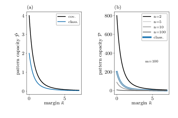
The pattern capacity decreases with the number of outputs.

Contrary to classical perceptrons, which have a pattern capacity independent of $n$ , the pattern capacity of the covariance perceptron decreases with increasing number $n$ of outputs (Figure 5b): $\mathcal{P}^{\mathrm{cov}}\sim(n-1)^{-1}$ . This can be understood as follows: For classical perceptrons, the weights to different readouts are independent. Therefore, adding more readouts does not impact the determination of possible weight configurations of the already existing readouts. The covariance perceptron, however, constitutes a bilinear mapping in terms of weights which leads to shared weight vectors for different output covariances. As an example, the weight vector for neuron $1$ impacts the output $Q_{1j}$ for all outputs $j>1$ . Thus, adding one more output, let’s say the $n$ -th output, to the covariance perceptron thereby imposes constraints on all $n-1$ other weight vectors to the already existing outputs. This causes the classification problem to become harder the more output covariances have to be tuned. It explains the decline in pattern capacity by a factor $n-1$ in Eq. (35). Overall, the covariance perceptron has superior pattern capacity in the case of $n<5$ outputs.

The information capacity exceeds that of the classical perceptron.

Although the covariance perceptron can classify less patterns than the classical perceptron in the case of many outputs, one has to take into account that each pattern has a much higher information content in the case of the covariance perceptron ( $m(m-1)/2$ vs $m$ bits in the input and $n(n-1)/2$ vs $n$ bits in the output). The information capacity, that is the amount of bits a classical computer would need to store a lookup table to implement the same classification as performed by the covariance perceptron, is (with $K=2^{m(m-1)/2}$ , $L=2^{n(n-1)/2}$ ) given by

\displaystyle\mathcal{I}^{\mathrm{cov}}(\kappa)

\displaystyle=

\displaystyle\mathcal{P}^{\mathrm{cov}}(\kappa)\left(m(m-1)/2+n(n-1)/2\right).

Note that we here, for simplicity, considered the case $f=1$ (which in general breaks the positive definiteness of the covariance patterns). The general case $f\neq 1$ is discussed in Section 6.3. We notice that the expression for the information capacity of the covariance perceptron grows $\propto m^{2}(m-1)/(n-1)$ , while the former for the classical perceptron grows with $m^{2}$ (Eq. 7).

In the brain, each neuron makes up to thousands of connections. Therefore, connections are the main objects that cost space. In addition, the number of synaptic events per time is a common measure for energy consumption. An important measure for classification performance is, therefore, the information capacity per synapse $\hat{\mathcal{I}}$ (Figure 6). For this measure, we get

\displaystyle\frac{\hat{\mathcal{I}}^{\mathrm{cov}}(\kappa)}{\hat{\mathcal{I}}^{\mathrm{class}}(\kappa)}

\displaystyle=

\displaystyle\frac{\mathcal{I}^{\mathrm{cov}}(\kappa)}{\mathcal{I}^{\mathrm{class}}(\kappa)}\mathrel{{\mathop{\approx}\limits}}\left\{\begin{array}[]{cc}2&,n\gg m\\ 2&,n=m\\ 2\frac{m-1}{n-1}&,n\ll m\end{array}\right.

For a network with $m=n$ , we get $\hat{\mathcal{I}}^{\mathrm{cov}}(\kappa)\approx 2\hat{\mathcal{I}}^{\mathrm{class}}(\kappa)$ , i.e. a two times larger information capacity than for the classical perceptron (Figure 6b). The same is true if the number of outputs is much larger than the number of inputs. However, for networks with strong convergence, i.e. $n\ll m$ , the covariance perceptron outperforms the classical perceptron by a factor $2(m-1)/(n-1)$ that can be potentially very large (Figure 6). Note that a similar result holds for different levels of sparsity (see Section 6.3, Figure 6a). Therefore, in networks that perform a strong compression of inputs, the covariance perceptron much more efficiently uses its connections to store information about the stimuli.

The numerical solution is an NP-hard problem

To check the prediction by the theory, we compare it to numerical experiments. The problem of finding the weight vectors can be formulated as maximizing the margin given a certain pattern load. This approach is the same as for the classical perceptron: Here, the training can be reduced to a quadratic programming problem [27, eq. 10.3], the minimization of the length of the readout vector under the constraints that all patterns be classified with unit margin.

Since the margin $\kappa$ is a non-analytic function due to the appearance of the minimum operation (1), it cannot be used directly to perform a gradient descent with regard to the weights. We thus employ an analytical approximation of the margin, the soft-margin

\kappa_{\eta}:=-\frac{1}{\eta}\,\ln\,\left(\sum_{r}^{p}\sum_{s}^{N}\,\exp\big(-\eta\,\zeta_{s}^{r}G_{s}^{r}\big)\right),

which covaries with $\kappa=\lim_{\eta\rightarrow\infty}\kappa_{\eta}$ , and can be optimized via a standard gradient ascent (see Section 6.1). Physically this soft-margin can be interpreted as a system at finite inverse temperature $\eta$ for which we find the set of parameters, the weight vectors, which maximize the free energy $\kappa_{\eta}$ . The states of the system here comprise a discrete set, given by the patterns $\{\zeta^{r}P^{r}\}_{r}$ . In the limit of vanishing temperature, $\eta\to\infty$ , the soft-margin approaches the true margin. It is also obvious, by Hoelder’s inequality, that the soft-margin is convex in each of the two weight vectors.

The resulting capacity curve is shown in Figure 7a. We observe that the achieved margin is well below the theoretical prediction. A better numerical implementation follows from a formulation as a quadratically constrained quadratic programming problem (cf. Section 6.2). For general constraints, these problems are typically NP-hard. Using an approximate procedure that iteratively improves an initial guess (alternating directions method of multipliers (ADMM), [28]), yields a margin that is comparable to the solution obtained by the gradient ascent for low pattern loads and slightly superior for larger pattern loads, as shown in Figure 7. As the load increases beyond the point $\hat{\mathcal{P}}\gtrsim 2$ , the method typically does not find a solution anymore; a large fraction of patterns have a negative margin and are thus classified wrongly (Figure 7b). Employing, instead, an interior point optimizer (IPOPT, [29]) yields a significantly larger margin for all pattern loads up to $\hat{\mathcal{P}}\approx 3$ , where this scheme breaks down (Figure 7b). The result of the interior point optimizer compares well to the theoretical prediction in the regime of low pattern load. For larger loads, the numerically found margin, however, is still slightly smaller than predicted by the replica-symmetric mean-field theory. Running the optimization for different initial conditions results in slightly different results for the margin (only the maximal one is shown in Figure 7a) indicating that the optimizer does not reliably find the unique solution that is predicted by the theory.

5 Discussion

In this work, we study information processing of networks that, like biological neural networks, process temporal signals. We investigate the scenario where the input-output mapping is dominated by the linear response, which is a good approximation for small signals in the typical dynamical regime of cortical networks [30, 16]. Focusing only on the temporal mean of these signals, such networks act as a classical perceptron if a classification threshold is applied to the outputs. Covariances of small temporal signals, however, transform in a bilinear fashion in terms of weights, giving rise to what we call a ’covariance perceptron’. The presented theoretical calculations focus on the pattern and information capacities of such a covariance perceptron. The theory uses Gardner’s theory of connections [19] in the thermodynamic limit, toward infinitely many inputs ( $m\to\infty$ ). We have shown that the covariance perceptron indeed presents an analytically solvable model in this limit and compute the pattern capacity by replica symmetric mean-field theory, analogous to the classical perceptron [19]. It turns out that the pattern capacity exceeds that of the classical perceptron for a single readout covariance ( $n=2$ ), whereas it decreases in the case of many outputs. The information capacity in bits of the covariance perceptron grows with $m^{2}(m-1)/(n-1)$ , whereas it only has a dependence as $m^{2}$ for the classical perceptron. The proposed paradigm in large and strongly convergent networks can therefore reach an information capacity that is orders of magnitude higher than that of the classical perceptron.

The dependence of the pattern capacity on the number of readout neurons $n$ is a non-trivial result in the case of the covariance perceptron, because different entries $Q_{ij}$ here share the same rows of the matrix $W$ . These partly confounding constraints reduce the capacity from the naively expected independence of the $n(n-1)/2$ readouts to a factor $(n-1)^{-1}$ . This factor signifies that with increasing numbers of readouts, the number of potentially confounding requirements on the readout vectors rises. Likewise, the capacity cannot simply be estimated by counting numbers of free parameters.

We demonstrate in [15] that the paradigm of classification that we analyzed here can indeed be implemented by means of a network of linear autoregressive processes. In particular, it is possible to derive learning rules that are local in time, which tune the readout vectors for binary classification of covariance patterns. Estimating covariance patterns from a time series naturally requires the observation of the process for a certain duration. The resulting estimation noise can be shown not to be detrimental for the performance of the classification [15]. The gradient-based learning rule derived in [15] does not reach as superior performance for single readouts as derived in this manuscript. The reason is twofold: 1. Gardner’s theory predicts the theoretical optimum for the capacity, but it is agnostic to the learning process that should reach this optimum. Any biophysical implementation of the learning therefore is likely to yield worse performance. 2. The non-biophysical learning by gradient-based soft-margin optimization studied here is also incapable of reaching the theoretical optimum, showing that gradient-based methods struggle with the non-convexity of the optimization problem. Yet, the learning rule in [15] yields as good results as for the classical perceptron.

The seminal work by Gardner [19] spurred many applications and extensions. For example, the information capacity within the error regime [31] or the computation of the distribution of synaptic weights of the Purkinje cell [32]. Recently, the theory has been extended to the classification of data points that possess a manifold structure [33]. So far, these works employed a linear mapping prior to the threshold operation. Here we turn to bilinear mappings in terms of weights and show their tight relation to the classical perceptron, but expose also striking differences. The bilinear mapping that we considered arose here from the mapping of covariance matrices by a linear network dynamics.

The reduction of dimensionality of covariance patterns —from many input nodes to a few output nodes— implements an “information compression”. For the same number of input-output nodes in the network, the use of covariances instead of means makes a higher-dimensional space accessible to represent input and output, which may help in finding a suitable projection for a classification problem. It is worth noting that applying a classical machine-learning algorithm, like the multinomial linear regressor [34], to the vectorized covariance matrices corresponds to $nm(m-1)/2$ weights to tune, to be compared with only $nm$ weights in our study (with $m$ inputs and $n$ outputs).

The presented calculations are strictly valid only in the thermodynamic limit $m\rightarrow\infty$ . The finite-size simulations that we presented here agree well, but also show differences to the theory. The discrepancies between the analytical prediction from the replica-symmetric mean-field theory and the numerically obtained optimization of the margin may have different sources. The first are true finite-size effects. Corrections would technically correspond to taking fluctuations of the auxiliary fields into account in addition to their saddle point values. A qualitatively different source of discrepancy arises from the method of training that we devised here. We first used a gradient ascent of a soft-margin. The latter only approximately agrees to the true margin. Also, as the training is implemented by a gradient ascent of the margin, stopping too early at large system size may lead to an underestimation of the theoretically possible margin. Analogous to classical perceptron learning, which, formulated as a support vector machine, can be recast into a quadratic programming problem [27], the covariance perceptron maps to a quadratically constrained quadratic programming problem. These problems are in general NP hard, so that training time increases exponentially with system size. It is clear that the complexity of the optimization problem increases with pattern load, because each pattern contributes one additional inequality constraint. The observed deviations appear at a pattern load of $\mathcal{P}\gtrsim 3$ . It is likely that they are due to the inability of the numerical solver to identify the unique optimal solution.

Another possibility is that indeed multiple solutions with similar margins exist if the load exceeds a certain point. This situation would correspond to replica symmetry breaking, because the existence of multiple degenerate solutions for the readout vector would show up as different replica settling in either of these solutions; analogous to a disordered system, which possesses a number of nearly degenerate meta-stable ground states [23]. In Gardner’s theory we search for the point at which the overlap between replica becomes unity; this assumption would have to be relaxed. It is conceivable that instead the set of these solutions vanishes together as the pattern load is increased beyond the capacity limit. Future work should address this question, either by the application of more powerful numerical optimizers or by analyzing the replica-symmetric mean-field theory with regard to instabilities of the symmetric solution.

The analysis presented here assumed the classification of uncorrelated patterns. In applications, however, the data to be classified typically has some internal structure. In the simplest case, different patterns could be correlated with correlations of a certain order. Second order correlations between patterns, for example, would show up in the pattern average (15) as additional quadratic terms, which would require the introduction of additional auxiliary fields for decoupling. A detailed analysis of this extension is left for future work.

The approximation of the network mapping in linear response theory here leads to a straight forward relationship between input and output covariances that is bilinear in the feed-forward connectivity matrix. In recurrent networks, linear response theory would amount to determining the network propagator. Such mappings are of the form $W(\omega)=(1+H(\omega)\,J)^{-1}$ , where $H(\omega)$ is the Fourier transform of the temporal linear response kernel of a neuron and $J$ the recurrent connectivity. This expression shows that the mapping between input and output covariances becomes more involved in the recurrent setting. Analyzing this situation may be possible by expressing the matrix inversion that appears in the propagator by help of a Gaussian integral. We leave this problem open for future work. An alternative approach first determines the optimal bilinear readout, as presented here, and subsequently determines the parameters of the recurrent network, foremost its connectivity, to implement this mapping.

Another extension consists in considering patterns of higher-than-second-order correlations. Generalizing the obtained results, higher-dimensionality may lead to higher information capacity when large number of inputs are considered. In contrast, this also implies additional constraints that limit the information capacity as shown when increasing the number of outputs for the present case of second-order correlations. There should thus be a trade-off for optimal information capacity that depends on the correlation order and the number of inputs and outputs.

Going beyond linear response theory is another route that may lead to a problem of similar structure as the system studied here. Concretely, assume the simplest setting of a static input-output mapping described by a quadratic gain function $y=f(z)=z^{2}$ of a neuron. When mapping the summed synaptic input $z_{i}=\sum_{k}w_{ik}x_{k}$ , the mean of the output $Y_{i}=\big[W\tilde{P}W^{\mathrm{T}}\big]_{ii}$ contains a bilinear term in $W$ that maps the matrix of second moments $\tilde{P}$ of the data to the first moment of the network’s output. This mapping is similar to the one studied here. A difference is, though, the dimension of the output, which in the latter case equals the number of units. Analyzing this system may be an interesting route for future studies.

A central motivation to study the current setting comes from the need to derive a self-consistent theory of biological information processing. As learning at the synaptic level is implemented by covariance-sensitive learning rules, using a covariance-based representation of information thus allows the construction of a scheme that is consistent at all levels. A further crucial ingredient would be the study of the covariance mapping across multiple layers of processing and including the abundant presence of recurrence.

This work was partially supported by the Marie Sklodowska-Curie Action (Grant H2020-MSCA-656547) of the European Commission, the Helmholtz young investigator’s group VH-NG-1028, the European Union’s Horizon 2020 research and innovation programme under grant agreement No. 785907 (Human Brain Project SGA2), the Exploratory Research Space (ERS) seed fund neuroIC002 (part of the DFG excellence initiative) of the RWTH university and the JARA Center for Doctoral studies within the graduate School for Simulation and Data Science (SSD).

6 Appendix

6.1 Optimization of the soft-margin

In order to numerically test the theoretical predictions, we need to maximize Eq. (1). A gradient-based optimization is, however, unfeasible due to the non-analytical minimum operation. Therefore, as an alternative, we consider the following soft-minimum as an objective function

	$\displaystyle O(W)$	$\displaystyle:=$	$\displaystyle-\kappa_{\eta}(W)=\frac{1}{\eta}\,\ln\,\left(\sum_{r=1}^{p}\,\sum_{i<j}\,\exp\big(-\eta\,\zeta_{ij}^{r}(WP^{r}W^{\mathrm{T}})_{ij}\big)\right)$		(42)
		$\displaystyle=$	$\displaystyle\frac{1}{\eta}\,\ln\,\left(\sum_{r=1}^{p}\,\frac{1}{2}\sum_{i\neq j}\,\exp\big(-\eta\,\zeta_{ij}^{r}(WP^{r}W^{\mathrm{T}})_{ij}\big)\right).$		(42)

This definition has the form of a scaled (scaling parameter $\eta$ ) cumulant-generating function, if we consider the patterns to be drawn randomly. In the limit $\eta\to\infty$ , this objective function will be dominated by the points with the smallest margins, so we recover

\kappa_{\eta}(W)\mathrel{{\mathop{\to}\limits}}\min_{ij,r}\,\big(\zeta_{ij}^{r}(WP^{r}W^{\mathrm{T}})_{ij}\big).

(43)

We use this objective function $O(W)$ with finite $\eta$ : Larger $\eta$ causes stronger contribution of patterns classified with small margin.

In order to check the analytical prediction for the maximum pattern capacity $\mathcal{P}$ (Figure 7), we need to find

W_{\mathrm{opt}}=\arg\min_{W}O(W).

(44)

We solve the minimization problem by gradient descent, which yields, with $\zeta_{ij}^{r}(WP^{r}W^{\mathrm{T}})_{ij}=\zeta_{ij}^{r}\,\sum_{kl}^{m}W_{ik}P_{kl}^{r}W_{jl}$ , the gradient

$\displaystyle\frac{\partial O(W)}{\partial W_{uv}}$	$\displaystyle=$	$\displaystyle\frac{1}{\eta}\,\frac{\sum_{r}^{p}\,\frac{1}{2}\sum_{i\neq j}\,\frac{\partial A_{ij}^{r}}{\partial W_{uv}}}{\sum_{r}^{p}\,\frac{1}{2}\sum_{i\neq j}\,A_{ij}^{r}},$
$\displaystyle A_{ij}^{r}$	$\displaystyle=$	$\displaystyle\exp\big(-\eta\,\zeta_{ij}^{r}(WP^{r}W^{\mathrm{T}})_{ij}\big),$
$\displaystyle\frac{\partial A_{ij}^{r}}{\partial W_{uv}}$	$\displaystyle=$	$\displaystyle(-\eta\,\zeta_{ij}^{r})\,(\delta_{iu}\,\sum_{l}^{m}P_{vl}^{r}W_{jl}+\delta_{ju}\,\sum_{k}^{m}W_{ik}P_{kv}^{r})\,A_{ij}^{r}.$

We update the readout vectors by

\displaystyle\Delta W_{uv}

\displaystyle=

\displaystyle-\iota\,\frac{\partial O(W)}{\partial W_{uv}},

where $\iota>0$ is the learning rate, here set to be $\iota=0.01$ . The normalization of the readout vectors is taken care of by enforcing unit length after each learning step (Figure 8).

6.2 Formulation as quadratically-constrained quadratic programming problem

To obtain a numerical solution for the covariance perceptron, it is convenient to reformulate the optimization problem in the form of a quadratically constrained quadratic programming problem. These problems frequently occur in different fields of science and efficient numerical solvers exist. The idea is analogous to the formulation of the support vector machine learning in terms of a quadratic programming problem [27, eqs. (10.3) and (10.4)]. For $n=2$ , an equivalent problem to finding the bi-linear readout with unit-length readout vectors $w_{i}\in\mathbb{R}^{n}$ , $i=1,2$ that maximize the margin, is the optimization problem

	$\displaystyle\text{minimize}:$		$\displaystyle\|\|\tilde{w}_{1}\|\|^{2}$
	with constraints:
			$\displaystyle\|\|\tilde{w}_{1}\|\|^{2}=\|\|\tilde{w}_{2}\|\|^{2},$
			$\displaystyle\zeta_{12}^{r}\tilde{w}_{1}^{\mathrm{T}}P^{r}\tilde{w}_{2}\geq 1\quad\forall\,1\leq r\leq p.$

The constraints can be formulated conveniently by combining the pair of readout vectors into a single vector $v=(\tilde{w}_{1},\tilde{w}_{2})\in\mathbb{R}^{2n}$ and defining for the length constraint a matrix

\displaystyle A_{ij}

\displaystyle:=

\displaystyle\left\{\begin{array}[]{cc}\delta_{ij}&1\leq i\leq n\\ -\delta_{ij}&n<i\leq 2n\end{array}\right.,

so that a pair of quadratic form inequality constraints $v^{\mathrm{T}}Av\geq 0$ and $v^{\mathrm{T}}Av\leq 0$ fixes the length of the two readout vectors to be identical. Analogously one defines for each pattern $r$ one matrix and a bi-linear inequality constraint to enforce a margin of at least unity as

	$\displaystyle B_{ij}^{r}$	$\displaystyle:=$	$\displaystyle\frac{1}{2}\left(\begin{array}[]{cc}0&\zeta^{r}P^{r}\\ \zeta^{r}(P^{r})^{\mathrm{T}}&0\end{array}\right),$
	$\displaystyle v^{\mathrm{T}}Bv$	$\displaystyle\geq$	$\displaystyle 1.$

The transposition of the matrix $(P^{r})^{\mathrm{T}}$ appearing in the lower left element, for symmetric matrices (covariances), can of course be left out. But the formulation also holds for non-symmetric matrices. The task is thus to minimize the norm of $v$ under $p+2$ quadratic inequality constraints. Random vectors with independent Gaussian entries, normalized to unit length, serve as initial guess. The normalized readout vectors are finally obtained as $w_{i}=\tilde{w}_{i}/||\tilde{w}_{i}||$ .

We here use an interior point method implemented in the package IPOPT [29], with a frontend provided by the python package QCQP [28] within the domain-specific language CVXPY [35].

6.3 Information capacity for sparse patterns

The number of configurations of a sparse covariance pattern is

K=\left(\begin{array}[]{c}M\\ fM\end{array}\right)2^{fM},

(47)

where $\left(\begin{array}[]{c}M\\ fM\end{array}\right)$ is the number of ways to position $fM$ non-zero entries in a single pattern of length $M$ , and $2^{fM}$ is the number of configurations of the non-zero entries in a single pattern. The information capacity follows as

	$\displaystyle\mathcal{I}^{\mathrm{cov}}(\kappa)$	$\displaystyle=$	$\displaystyle\mathcal{P}^{\mathrm{cov}}(\kappa)\left[fM+\log_{2}\left(\begin{array}[]{c}M\\ fM\end{array}\right)+N\right]$
		$\displaystyle\approx$	$\displaystyle\mathcal{P}^{\mathrm{cov}}(\kappa)\left[M(f-S(f))+N\right]$

where we used $\log_{2}\left(\begin{array}[]{c}M\\ fM\end{array}\right)=-MS(f)$ with $S(f)=\left(f\log_{2}(f)+(1-f)\log_{2}(1-f)\right)$ . Although the calculations in Section 3 ignore the constraint that the covariance matrices $P^{r}$ must be positive semidefinite, this constraint is ensured when using not too dense and strong entries such that $fc\ll 1$ , thanks to the unit diagonal. Since $\sqrt{fc^{2}}$ only determines the scale on which the margin $\kappa$ is measured, the optimal capacity can always be achieved if one allows for a sufficiently small margin. As shown in Figure 6b, the level of sparsity only has a minor impact on the information capacity per synapse when comparing to the classical perceptron.

References

[1] Rosenblatt F 1958 Psychol. Rev. 65 386–408
[2] Minsky M L and Papert S A 1969 Perceptrons (Cambridge: Cambridge MIT Press)
[3] Widrow B and Hoff M E 1960 Adaptive switching circuits 1960 IRE WESCON Convention Record (Part 4) (Los Angeles, CA: IRE) pp 96–104
[4] Hubel D H and Wiesel T N 1959 J. Physiol. 148 574–591
[5] Arieli A, Sterkin A, Grinvald A and Aertsen A 1996 Science 273 1868–1871
[6] Riehle A, Grün S, Diesmann M and Aertsen A 1997 Science 278 1950–1953
[7] Kilavik B E, Roux S, Ponce-Alvarez A, Confais J, Grün S and Riehle A 2009 J. Neurosci. 29 12653–12663
[8] Hebb D O 1949 The organization of behavior: A neuropsychological theory (New York: John Wiley & Sons)
[9] Hertz J, Krogh A and Palmer R G 1991 Introduction to the Theory of Neural Computation (Cambridge, MA: Perseus)
[10] Oja E 1982 J. Math. Biol. 15 267–273.
[11] Barak O and Tsodyks M 2006 Neural Comput. 18 2343–2358
[12] Gerstner W, Kempter R, van Hemmen J L and Wagner H 1996 Nature 383 76–78
[13] Markram H, Lübke J, Frotscher M and Sakmann B 1997 Science 275 213–215
[14] Bi G and Poo M 1998 J. Neurosci. 18 10464–10472
[15] Gilson M, Dahmen D, Moreno-Bote R, Insabato A and Helias M 2019 (bioRxiv:562546)
[16] Lindner B, Doiron B and Longtin A 2005 Phys. Rev. E 72 061919
[17] Grytskyy D, Tetzlaff T, Diesmann M and Helias M 2013 Front. Comput. Neurosci. 7 131
[18] Dahmen D, Grün S, Diesmann M and Helias M 2019 Proc. Natl. Acad. Sci. USA 116(26)
[19] Gardner E 1988 J. Phys. A: Math. Gen. 21 257
[20] Cortes C and Vapnik V 1995 Machine Learning 20 273–297
[21] Pernice V, Staude B, Cardanobile S and Rotter S 2011 PLOS Comput. Biol. 7 e1002059
[22] Trousdale J, Hu Y, Shea-Brown E and Josic K 2012 PLOS Comput. Biol. 8 e1002408
[23] Fischer K and Hertz J 1991 Spin glasses (Cambridge University Press)
[24] van Vreeswijk C and Sompolinsky H 1996 Science 274 1724–1726
[25] Renart A, De La Rocha J, Bartho P, Hollender L, Parga N, Reyes A and Harris K D 2010 Science 327 587–590
[26] Tetzlaff T, Helias M, Einevoll G T and Diesmann M 2012 PLOS Comput. Biol. 8 e1002596
[27] Vapnik V N 1998 Statistical learning theory (New York: Wiley)
[28] Park J and Boyd S 2017 General heuristics for nonconvex quadratically constrained quadratic programming (arXiv:1703.07870)
[29] Wächter A and Biegler L T 2006 Mathematical Programming vol 106 (Heidelberg, Berlin, New York: Springer) pp 25–57
[30] Brunel N 2000 J. Comput. Neurosci. 8 183–208
[31] Brunel N, Nadal J P and Toulouse G 1992 J. Phys. A: Math. Gen. 25 5017
[32] Brunel N, Hakim V, Isope P, Nadal J P and Barbour B 2004 Neuron 43 745–757
[33] Chung S, Lee D D and Sompolinsky H 2018 Phys. Rev. X 8 031003
[34] Bishop C M 2006 Pattern Recognition and Machine Learning (New York: Springer)
[35] Diamond S and Boyd S 2016 J. Mach. Learn. Res. 17 1–5