跳到论文正文
W Papers独立论文阅读器 arXiv:1912.00798 论文正文 计算阅读时间 · 0%
引用这篇论文根据当前论文元数据生成,正式投稿前建议核对。


License: arXiv.org perpetual non-exclusive license
arXiv:1912.00798v1 [math.PR] 29 Nov 2019

Equivalence of the Hazard Rate and Usual Stochastic Orders for Parallel Systems

Khaled Masoumifard Address: Department of Statistics, Faculty of Mathematical Sciences, Shahid Beheshti University, Tehran, Iran
Abstract

In this paper, we investigate stochastic comparisons of parallel systems, and obtain two characterization results in this regard. First, we compare a parallel system with independent heterogeneous components to a parallel system with homogeneous components, and establish some certain assumptions under which the hazard rate and usual stochastic orders between the lifetimes of two parallel systems are equivalent. Next, we turn our attention to two parallel systems with their component lifetimes following multiple-outlier model and prove that under some specified assumptions, the pp-larger order between the vectors of scale parameters is equivalent to the hazard rate order as well as the usual stochastic order between the lifetimes of these systems. The results established here are applicable to compute an upper bound for the hazard rate function and a lower bound for the survival function of a parallel systems consisting of heterogeneous components.

Keywords: 
Exponentiated Generalized Gamma Distribution, Power-generalized Weibull Distribution, Multiple-Outlier, Scale Model, Hazard Rate Order, Usual Stochastic Order, Hazard Rate Function, PP-Larger Order, Parallel System
2010 MSC
60E15, 60K10

1 Introduction

Consider a system with nn components, and assume this system fails if and only if at least kk components fail. Such a system is said to be an (n−k+1n-k+1)-out-of-nn system. Series and Parallel structures corresponding to nn-out-of-nn and 11-out-of-nn systems, respectively, appear extensively in the practice. In reliability theory, there exists an intimate relation between the (n−k+1n-k+1)-out-of-nn systems and the theory of order statistics. Suppose X1,⋯,XnX_{1},\cdots,X_{n} denote the lifetimes of components of a system and X1:n≤⋯≤Xn:nX_{1:n}\leq\cdots\leq X_{n:n} represent the corresponding order statistics. Then, the lifetime of an (n−k+1n-k+1)-out-of-nn system comprising these components coincides with the kk-th order statistic Xk:nX_{k:n}. By using the theory of order statistics, many properties of (n−k+1n-k+1)-out-of-nn systems have been established in the literature. Order statistics also play an importance role in various fields of probability and statistics; see, for example,[Arnold_1992] and [David_Nagaraja_2003].

1.1 Scale model

A set of independent random variables X1,⋯,XnX_{1},\cdots,X_{n} with respective distribution functions F1,⋯,FnF_{1},\cdots,F_{n} is said to follow the scale family model, if there exist positive constants λ1,⋯,λn\lambda_{1},\cdots,\lambda_{n} and an absolutely continuous distribution function FF, with corresponding density function ff, such that Fi​(x)=F⁡(λi​x)F_{i}(x)=F(\lambda_{i}x) for i=1,⋯,ni=1,\cdots,n. In this case, FF is called the baseline distribution, ff is called the baseline density and λ1,⋯,λn\lambda_{1},\cdots,\lambda_{n} are scale parameters. Let fif_{i} denote the density functions of XiX_{i}, i=1,⋯,ni=1,\cdots,n, then we have fi​(x)=λi​f​(λi​x)f_{i}(x)=\lambda_{i}\,f(\lambda_{i}x), i=1,⋯,ni=1,\cdots,n. Some well-known distributions such as normal, Weibull, gamma and generalized gamma are special cases of the scale model. For this reason, the scale model has received considerable attention in the statistical literature. One may refer to Chapters 7 and 16 of [Marshall_Olkin_2007] for more details on the scale model and its applications.

1.2 Exponentiated scale model

Suppose F(.)F(.) is a specified distribution with survival F¯(.)\bar{F}(.), hazard rate r(.)r(.) and reversed hazard rate r~(.)\tilde{r}(.), and α\alpha is a positive number. Set G⁡(x)=[F⁡(x)]αG(x)=[F(x)]^{\alpha}. Then, it is easy to observe that G(.)G(.) is also a distribution function. In this case, we say that FF is exponentiated by α\alpha. If r~G(.)\tilde{r}_{G}(.) denotes the reversed hazard rate function corresponding to GG, then we have r~G​(x)=α​r~F​(x)\tilde{r}_{G}(x)=\alpha\tilde{r}_{F}(x), which is referred to as the proportional reversed hazard rate or resilience model in the literature (see [Marshall_Olkin_2007], p. 234);

By using the exponentiation method, one can produce a new distribution with some attractive properties. For example, suppose F⁡(x)=1−e−xF(x)=1-e^{-x}, x>0x>0, and α\alpha is a positive number. Then, G⁡(x)=(1−e−x)αG(x)=(1-e^{-x})^{\alpha}, x>0x>0, is also a distribution function, which is called the generalized exponential distribution. It is well-known that the exponential distribution has constant hazard rate whereas the generalized exponential distribution has decreasing hazard rate for α≤1\alpha\leq 1 and increasing hazard rate for α≥1\alpha\geq 1. For a comprehensive discussion on the generalized exponential distribution, one may refer to [Gupta_Kundu_(1999)], [Gupta_Kundu_(2004)].

Suppose F(.)F(.) is an absolutely continuous distribution function with corresponding density f(.)f(.). Then, independent random variables X1,⋯,XnX_{1},\cdots,X_{n} are said to belong to the exponentiated scale family of distributions if Xi∼(F⁡(λi​x))αiX_{i}\sim\Big(F(\lambda_{i}\,x)\Big)^{\alpha_{i}}, where αi>0\alpha_{i}>0 and λi>0\lambda_{i}>0 for i=1,⋯,ni=1,\cdots,n. In this case, F(.)F(.) is said to be the baseline distribution function and αi\alpha_{i}’s and λi\lambda_{i}’s are the shape and scale parameters, respectively. Note that we can present the parameters of the exponentiated scale model in a matrix format.

Let us quickly recall some common notions of stochastic order, and majorization and pp-larger orders that will be used to establish the main results of the paper. Throughout, we use ‘increasing’ to state ‘non-decreasing’ and similarly ‘decreasing’ to state ‘non-increasing’. Suppose XX and YY are two non-negative random variables with distribution functions FF and G,G, survival functions F¯\bar{F} and G¯,\bar{G}, density functions ff and g,g, and hazard rates rX=f/F¯r_{X}=f/\bar{F} and rY=g/G¯,r_{Y}=g/\bar{G}, respectively. Then, XX is said to be larger than YY in the usual stochastic order (shown by X≥s​tYX\geq_{st}Y) iff F¯​(x)≥G¯​(x)\bar{F}(x)\geq\bar{G}(x) for all x∈ℝ+x\in\mathbb{R}^{+}. XX is said to be larger than YY in the hazard rate order (shown by X≥h​rYX\geq_{hr}Y) iff F¯​(x)/G¯​(x)\bar{F}(x)/\bar{G}(x) is increasing in x∈ℝ+x\in\mathbb{R}^{+}. In fact, X≥h​rYX\geq_{hr}Y iff rY​(x)≥rX​(x)r_{Y}(x)\geq r_{X}(x) for all x∈ℝ+x\in\mathbb{R}^{+}. It is well-known that the hazard rate order implies the usual stochastic order. Interested readers may refer to [Muller_Stoyan_(2002)] and [Shaked_Shanthikumar_(2007)] for comprehensive discussions on stochastic orders and their applications.

For two vectors 𝒙=(x1,⋯,xn)\mbox{\boldmath$x$}=(x_{1},\cdots,x_{n}) and 𝒚=(y1,⋯,yn)\mbox{\boldmath$y$}=(y_{1},\cdots,y_{n}), let {x(1),⋯,x(n)}\{x_{(1)},\cdots,x_{(n)}\} and {y(1),⋯,y(n)}\{y_{(1)},\cdots,y_{(n)}\} denote the increasing arrangements of their components, respectively. Then, the vector 𝒙x is said to majorize another vector 𝒚y (written 𝒙⪰m𝒚\mbox{\boldmath$x$}\stackrel{{\scriptstyle m}}{{\succeq}}\mbox{\boldmath$y$}) if ∑j=1ix(j)≤∑j=1iy(j)\,\sum_{j=1}^{i}\,x_{(j)}\leq\sum_{j=1}^{i}\,y_{(j)} for i=1,⋯,n−1i=1,\cdots,n-1, and ∑j=1nx(j)=∑j=1ny(j)\sum_{j=1}^{n}\,x_{(j)}=\sum_{j=1}^{n}\,y_{(j)}. The vector 𝒙x in ℝ+n\mathbb{R^{+}}^{n} is said to be pp-larger than another vector 𝒚y in ℝ+n\mathbb{R^{+}}^{n} (written 𝒙⪰p𝒚\mbox{\boldmath$x$}\stackrel{{\scriptstyle p}}{{\succeq}}\mbox{\boldmath$y$}) if ∏j=1ix(j)≤∏j=1iy(j)\,\prod_{j=1}^{i}\,x_{(j)}\leq\prod_{j=1}^{i}\,y_{(j)} for i=1,⋯,ni=1,\cdots,n. When 𝒙x,𝒚y in ℝ+n\mathbb{R^{+}}^{n}, 𝒙⪰m𝒚\mbox{\boldmath$x$}\stackrel{{\scriptstyle m}}{{\succeq}}\mbox{\boldmath$y$} implies 𝒙⪰p𝒚\mbox{\boldmath$x$}\stackrel{{\scriptstyle p}}{{\succeq}}\mbox{\boldmath$y$}. The converse is, however, not true. For example, (1,5.5)≥p(2,3)(1,5.5)\stackrel{{\scriptstyle p}}{{\geq}}(2,3), but clearly the majorization order does not hold between these two vectors. A real-valued function ϕ\phi, defined on a set 𝔸⊆ℝn\mathbb{A}\subseteq\mathbb{R}^{n}, is said to be Schur-convex (Schur-concave) on 𝔸\mathbb{A} if 𝒙⪰m𝒚\mbox{\boldmath$x$}\stackrel{{\scriptstyle m}}{{\succeq}}\mbox{\boldmath$y$} implies ϕ⁡(𝒙)≥(≤)​ϕ​(𝒚)\phi(\mbox{\boldmath$x$})\geq(\leq)\phi(\mbox{\boldmath$y$}) for any 𝒙,𝒚∈𝔸\mbox{\boldmath$x$},\mbox{\boldmath$y$}\in\mathbb{A}. For comprehensive discussions about the pp-larger and majorization orders with their applications, we refer the readers to Khaledi and [Kochar_(2002)] and [Marshall_et_al_(2011)].

In this paper, we compare parallel systems with respect to the hazard rate and usual stochastic orders when their components follow the exponentiated scale family of distributions. First, suppose X1,⋯,XnX_{1},\cdots,X_{n} are independent non-negative random variables with Xi∼(F⁡(λi​x))αiX_{i}\sim\bigg(F(\lambda_{i}x)\bigg)^{\alpha_{i}}, i=1,⋯,ni=1,\cdots,n, and suppose Y1,⋯,YnY_{1},\cdots,Y_{n} are independent non-negative random variables with common distribution function (F⁡(λ​x))αi\bigg(F(\lambda x)\bigg)^{\alpha_{i}}. Then, it is shown under some certain assumptions that

λ≥λw​g⟺Xn:n≥h​rYn:n⟺Xn:n≥s​tYn:n,\displaystyle\lambda\geq\lambda_{wg}\Longleftrightarrow X_{n:n}\geq_{hr}Y_{n:n}\Longleftrightarrow X_{n:n}\geq_{st}Y_{n:n}, (1.1)

where λw​g=∏i=1nλiαi/n​α¯\lambda_{wg}=\prod_{i=1}^{n}\lambda_{i}^{{\alpha_{i}}/{n\bar{\alpha}}} is the weighted geometric mean of λi\lambda_{i}’s. We show that the results in (1.1) hold for the power generalized weibull and exponentiated generalized gamma family of distributions. By means of a counterexample, we show that the result in (1.1) cannot be extended to the general case when the lifetimes of two parallel systems are heterogeneous and the vectors of scale parameters are ordered with respect to the pp-larger order. So, for extending (1.1), in the first step we turn our attention to the multiple-outlier scale model which reduces the complete heterogenity of the scale parameters. Specifically, suppose X1,⋯,XnX_{1},\cdots,X_{n} are independent non-negative random variables with Xi∼F⁡(λ​x)X_{i}\sim F(\lambda x), i=1,⋯,pi=1,\cdots,p, and Xj∼F⁡(λ∗​x)X_{j}\sim F(\lambda^{*}x), j=p+1,⋯,nj=p+1,\cdots,n. Further, suppose Y1,⋯,YnY_{1},\cdots,Y_{n} is another set of independent non-negative random variables with Yi∼F⁡(μ​x)Y_{i}\sim F(\mu x), i=1,⋯,pi=1,\cdots,p, and Yj∼F⁡(μ∗​x)Y_{j}\sim F(\mu^{*}x), j=p+1,⋯,nj=p+1,\cdots,n. Assume that λ≤μ≤μ∗≤λ∗\lambda\leq\mu\leq\mu^{*}\leq\lambda^{*}. Then, under some specified assumptions, we show that

(λ,⋯,λ⏟p,λ∗,⋯,λ∗⏟n−p)⪰p(μ,⋯,μ⏟p,μ∗,⋯,μ∗⏟n−p)⟺Xn:n≥h​rYn:n⟺Xn:n≥s​tYn:n.\displaystyle(\underbrace{\lambda,\cdots,\lambda}_{p},\underbrace{\lambda^{*},\cdots,\lambda^{*}}_{n-p})\stackrel{{\scriptstyle p}}{{\succeq}}(\underbrace{\mu,\cdots,\mu}_{p},\underbrace{\mu^{*},\cdots,\mu^{*}}_{n-p})\Longleftrightarrow X_{n:n}\geq_{hr}Y_{n:n}\Longleftrightarrow X_{n:n}\geq_{st}Y_{n:n}. (1.2)

We also show that the results in (1.2) hold for the power generalized weibull and generalized gamma family of distributions. The results established here reinforce and extend the well-known results in [Zhao_(2011)],[Zhao_Balakrishnan_(2012)], Balakrishnan and [Zhao_(2013a)] and [Balakrishnan_et_al_(2014)] which deal with the exponential, gamma and generalized exponential distributions.

2 Preliminaries

In this section, we discuss some aspects of the scale model and present some useful lemmas that will be used in the sequel. Suppose X1,⋯,XnX_{1},\cdots,X_{n} are independent non-negative random variables following the scale model with the scale parameters λ1⋯,λn,\lambda_{1}\cdots,\lambda_{n}, the baseline distribution F,F, and the baseline density ff. In this paper, we assume some certain assumptions on the baseline density to simplify the computation. More precisely, suppose the baseline density function can be rewritten as

f⁡(x)=w⁡(x)​h​(x),x∈ℝ+,\displaystyle f(x)=w(x)\,h(x),\qquad\quad x\in\mathbb{R^{+}}, (2.3)

where w⁡(x)w(x) and h⁡(x)h(x) are two differentiable positive functions with the following properties:
C-1.  w⁡(x​y)=w⁡(x)​w​(y)w(xy)=w(x)\,w(y) for all x,y∈ℝ+x,y\in\mathbb{R}^{+};
C-2.  limx→0h⁡(λi​x)h⁡(λj​x)=1\lim_{x\rightarrow 0}\frac{\displaystyle h(\lambda_{i}x)}{\displaystyle h(\lambda_{j}x)}=1.
As an example of the decomposition form in (2.3),

  • 1.

    set

    w⁡(x)=xp−1a​n​dh⁡(x)=pq​(1+xp)1q−1​e1−(1+xp)1q,x∈ℝ+,\displaystyle w(x)=x^{p-1}\qquad and\qquad h(x)=\frac{\displaystyle p}{\displaystyle q}(1+x^{p})^{\frac{1}{q}-1}e^{1-(1+x^{p})^{\frac{1}{q}}},\qquad x\in\mathbb{R^{+}},

    where p>0p>0, q>0q>0. Clearly, the assumptions in C-1 and C-2 satisfy for this case. Under this setting, the baseline density function reduces to the density function of the power generalized weibull distribution with shape parameters pp and qq, and scale parameter 1 (on in short P​G​W​(p,q,1)PGW(p,q,1)). The power generalized weibull distribution has a decreasing failure rate when p≤q,p≤1p\leq q,\,p\leq 1, an increasing failure rate when p≥q,p≥1p\geq q,\,p\geq 1, a bathtub failure rate when 0<q<p<10<q<p<1 and an upside down bathtub (or unimodal) failure rate when q>p>1q>p>1. It includes Weibull and exponential distributions as special cases. For more details on this family and its applications in probability and statistics,the reader is referred to [Bagdonavicius] and [Nikulin_(2002)].

  • 2.

    set

    w⁡(x)=xβ−1a​n​dh⁡(x)=αΓ∗​(βα)​e−xα,x∈ℝ+,\displaystyle w(x)=x^{\beta-1}\qquad and\qquad h(x)=\frac{\displaystyle\alpha}{\displaystyle\Gamma^{*}(\frac{\displaystyle\beta}{\displaystyle\alpha})}\,e^{-x^{\alpha}},\qquad x\in\mathbb{R^{+}},

    where α>0\alpha>0, β>0\beta>0, and Γ∗(.)\Gamma^{*}(.) indicates the gamma function. Clearly, the assumptions in C-1 and C-2 satisfy for this case. Under this setting, the baseline density function reduces to the density function of the generalized gamma distribution with shape parameters α\alpha and β\beta, and scale parameter 1 (on in short G​G​(α,β,1)GG(\alpha,\beta,1)). The generalized gamma distribution includes exponential, Weibull and gamma distributions as special cases. Moreover, the log-normal distribution can be also obtained from the generalized gamma distribution as α=2\alpha=2 and β→∞\beta\rightarrow\infty. The generalized gamma distribution also has a flexible hazard rate function which is increasing for α≥1\alpha\geq 1 and β≥1\beta\geq 1, decreasing for α≤1\alpha\leq 1 and β≤1\beta\leq 1, bathtub shape for α<1\alpha<1 and β>1\beta>1 and upside-down bathtub shape for α>1\alpha>1 and β<1\beta<1. For more details on the generalized gamma distribution and its applications, we refer the readers to [Balakrishnan_and_Peng_(2006)] and [Kleiber_Kotz_(2003)].

From the assumptions in C-1 and C-2, we easily obtain the following result.

Remark 2.1.

w⁡(1)=1w(1)=1 and w⁡(x)=xw′​(1)w(x)=x^{w^{\prime}(1)} for every x∈ℝ+x\in\mathbb{R}^{+}, where w′​(x)w^{\prime}(x) denote the derivative of w⁡(x)w(x) with respect to xx.

In the following lemma, we compare a parallel system consisting of components whose lifetimes follow the exponentiated scale model to the same system with lifetimes of its components following the homogeneous exponentiated scale model, and establish some certain assumptions under which the hazard rate and usual stochastic orders between the lifetimes of these systems are equivalent.

Lemma 2.1.

Suppose X1,⋯,XnX_{1},\cdots,X_{n} are independent non-negative random variables with Xi∼(F⁡(λi​x))αiX_{i}\sim\big(F(\lambda_{i}\,x)\big)^{{\alpha}_{i}}, i=1⋯,ni=1\cdots,n. Further, suppose Y1,⋯,YnY_{1},\cdots,Y_{n} are independent non-negative random variables with Yi∼(F⁡(λ​x))αiY_{i}\sim\big(F(\lambda x)\big)^{{\alpha}_{i}}. Assume that following assumptions hold:

  • (aa)

    x​r~​(x)x\tilde{r}(x) is decreasing in x∈ℝ+x\in\mathbb{R}^{+};

  • (bb)

    x​(r~​(x)−h′​(x)h⁡(x))x(\tilde{r}(x)-\frac{h^{\prime}(x)}{h(x)}) is increasing in x∈ℝ+x\in\mathbb{R}^{+};

  • (cc)

    F¯​(x)≤−w⁡(x)​h2​(x)h′​(x)\bar{F}(x)\leq-\frac{w(x)\,h^{2}(x)}{h^{\prime}(x)} for every x∈ℝ+x\in\mathbb{R}^{+}.

Where r~​(x)=f​(x)/F​(x)\tilde{r}(x)={f(x)}/{F(x)}. Then, for αi≥1,i=1,⋯,n\alpha_{i}\geq 1,\,i=1,\cdots,n the following three statements are equivalent:

  • (i)

    λ≥λw​g\lambda\geq\lambda_{wg};

  • (ii)

    Xn:n≥h​rYn:nX_{n:n}\geq_{hr}Y_{n:n};

  • (ii)

    Xn:n≥s​tYn:nX_{n:n}\geq_{st}Y_{n:n}.

Where λw​g=∏i=1nλiαi∑i=1nαi{\lambda}_{wg}=\prod_{i=1}^{n}\lambda_{i}^{\frac{\alpha_{i}}{\sum_{i=1}^{n}\alpha_{i}}}.

Now, we derive some ordering results between parallel systems with the lifetimes of their components following the exponentiated scale model under the decomposition form in (2.3) and the assumptions in C-1 and C-2.

Lemma 2.2.

Suppose X1,⋯,XnX_{1},\cdots,X_{n} are independent non-negative random variables with Xi∼F⁡(λ​x)X_{i}\sim F(\lambda x), i=1,⋯,pi=1,\cdots,p, and Xj∼F⁡(λ∗​x)X_{j}\sim F(\lambda^{*}x), j=p+1,⋯,nj=p+1,\cdots,n. Further, suppose Y1,⋯,YnY_{1},\cdots,Y_{n} is another set of independent non-negative random variables with Yi∼F⁡(μ​x)Y_{i}\sim F(\mu x), i=1,⋯,pi=1,\cdots,p, and Yj∼F⁡(μ∗​x)Y_{j}\sim F(\mu^{*}x), j=p+1,⋯,nj=p+1,\cdots,n. Assume that following assumptions hold:

  • (aa)

    x​r~​(x)x\tilde{r}(x) is decreasing in x∈ℝ+x\in\mathbb{R}^{+};

  • (bb)

    x​(r~​(x)−h′​(x)h⁡(x))x(\tilde{r}(x)-\frac{h^{\prime}(x)}{h(x)}) is increasing in x∈ℝ+x\in\mathbb{R}^{+};

  • (cc)

    F¯​(x)≤−w⁡(x)​h2​(x)h′​(x)\bar{F}(x)\leq-\frac{w(x)\,h^{2}(x)}{h^{\prime}(x)} for every x∈ℝ+x\in\mathbb{R}^{+}.

So, if λ≤μ≤μ∗≤λ∗\lambda\leq\mu\leq\mu^{*}\leq\lambda^{*} and λp​λ∗n−p=μp​μ∗n−p\lambda^{p}{\lambda^{*}}^{n-p}=\mu^{p}{\mu^{*}}^{n-p}, then Xn:n≥h​rYn:n.X_{n:n}\geq_{hr}Y_{n:n}.

Lemma 2.3.

Suppose X1,⋯,XnX_{1},\cdots,X_{n} are independent non-negative random variables with Xi∼F⁡(λ​x)X_{i}\sim F(\lambda x), i=1,⋯,pi=1,\cdots,p, and Xj∼F⁡(λ∗​x)X_{j}\sim F(\lambda^{*}x), j=p+1,⋯,nj=p+1,\cdots,n. Further, suppose Y1,⋯,YnY_{1},\cdots,Y_{n} is another set of independent non-negative random variables with Yi∼F⁡(μ​x)Y_{i}\sim F(\mu x), i=1,⋯,pi=1,\cdots,p, and Yj∼F⁡(μ∗​x)Y_{j}\sim F(\mu^{*}x), j=p+1,⋯,nj=p+1,\cdots,n. Assume that λ≤μ≤μ∗≤λ∗\lambda\leq\mu\leq\mu^{*}\leq\lambda^{*} and following assumptions hold:

  • (aa)

    x​r~​(x)x\tilde{r}(x) is decreasing in x∈ℝ+x\in\mathbb{R}^{+};

  • (bb)

    x​(r~​(x)−h′​(x)h⁡(x))x(\tilde{r}(x)-\frac{h^{\prime}(x)}{h(x)}) is increasing in x∈ℝ+x\in\mathbb{R}^{+};

  • (cc)

    F¯​(x)≤−w⁡(x)​h2​(x)h′​(x)\bar{F}(x)\leq-\frac{w(x)\,h^{2}(x)}{h^{\prime}(x)} for every x∈ℝ+x\in\mathbb{R}^{+}.

Then, the following three statements are equivalent:

  • (i)

    (λ,⋯,λ⏟p,λ∗,⋯,λ∗⏟n−p)⪰p(μ,⋯,μ⏟p,μ∗,⋯,μ∗⏟n−p)(\underbrace{\lambda,\cdots,\lambda}_{p},\underbrace{\lambda^{*},\cdots,\lambda^{*}}_{n-p})\stackrel{{\scriptstyle p}}{{\succeq}}(\underbrace{\mu,\cdots,\mu}_{p},\underbrace{\mu^{*},\cdots,\mu^{*}}_{n-p});

  • (ii)

    Xn:n≥h​rYn:nX_{n:n}\geq_{hr}Y_{n:n};

  • (iii)

    Xn:n≥s​tYn:nX_{n:n}\geq_{st}Y_{n:n}.

3 Comparison of Xn:nX_{n:n} from Heterogenous and Homogeneous Samples

Stochastic comparisons of a parallel system with independent heterogeneous components to a parallel system with homogeneous components were first made by [Dykstra_et_al] Let (X1,⋯,Xn)(X_{1},\cdots,X_{n}) and (Y1,⋯,Yn)(Y_{1},\cdots,Y_{n}) be two independent random vectors,

  • 1.

    If Xi∼E⁡(λi)X_{i}\sim E(\lambda_{i})11 1 Exponential distribution with hazard rate λi\lambda_{i} and Yi∼E⁡(λ)Y_{i}\sim E({\lambda}), i=1,⋯,ni=1,\cdots,n, [Dykstra_et_al] showed that

    λ=λ¯⟹Xn:n≥h​rYn:n\displaystyle\lambda=\bar{\lambda}\Longrightarrow X_{n:n}\geq_{hr}Y_{n:n} (3.4)

    where λ¯=1n​∑i=1nλi\bar{\lambda}=\frac{1}{n}\sum_{i=1}^{n}\lambda_{i}, the arithmetic mean of λi\lambda_{i}’s. Which was further strengthened by [kochar2007some] as

    Xn:n≥l​rYn:n.X_{n:n}\geq_{lr}Y_{n:n}.

    [10] also strengthened the result in (3.4), under a weaker condition,

    λ=λ~⟹Xn:n≥h​rYn:n\lambda=\tilde{\lambda}\Longrightarrow X_{n:n}\geq_{hr}Y_{n:n}

    where λ~=(∏i=1nλi)1/n\tilde{\lambda}=\bigg(\prod_{i=1}^{n}\lambda_{i}\bigg)^{1/n}, the geometric mean of λi\lambda_{i}’s.

  • 2.

    If Xi∼G⁡(r,λi)X_{i}\sim G(r,\lambda_{i})22 2 Gamma distribution with shape parameter rr and scale parameter λi\lambda_{i} and Yi∼G⁡(r,λ~)Y_{i}\sim G(r,\tilde{\lambda}), i=1,⋯,ni=1,\cdots,n, [balakrishnan2013hazard] show that, for 0<r≤10<r\leq 1,

    Xn:n≥h​rYn:n.X_{n:n}\geq_{hr}Y_{n:n}.
  • 3.

    If Xi∼G​E​(αi,λi)X_{i}\sim GE(\alpha_{i},\lambda_{i})33 3 Generalized Exponential distribution with shape parameter αi\alpha_{i} and scale parameter λi\lambda_{i} and Yi∼G​E​(α¯,λw​g)Y_{i}\sim GE(\bar{\alpha},{\lambda_{wg}}), i=1,⋯,ni=1,\cdots,n, [balakrishnan2015stochastic] show that, for α¯≥1\bar{\alpha}\geq 1,

    Xn:n≥h​rYn:nX_{n:n}\geq_{hr}Y_{n:n}

    where α¯=1n​∑i=1nαi\bar{\alpha}=\frac{1}{n}\sum_{i=1}^{n}\alpha_{i} and λw​g=∏i=1λiαi/n​α¯\lambda_{wg}=\prod_{i=1}\lambda_{i}^{{\alpha_{i}}/{n\bar{\alpha}}}. They also showed that, If Xi∼G​E​(α,λi)X_{i}\sim GE(\alpha,\lambda_{i}) and Yi∼G​E​(α,λ¯)Y_{i}\sim GE({\alpha},\bar{\lambda}), i=1,⋯,ni=1,\cdots,n, then

    Xn:n≥l​rYn:n.X_{n:n}\geq_{lr}Y_{n:n}.

The case of power-generalized weibull distribution and exponentiated generalized gamma distribution are discussed in the following subsections, respectively.

3.1 Power-generalized weibull distribution

In the following lemma, we show that the assumptions of Lemma 2.1 hold for the power-generalized weibull distribution under a restriction on its shape parameter.

Lemma 3.1.

Suppose the baseline distribution is P​G​W​(p,q,1)PGW(p,q,1). Then, for q≤1q\leq 1, the assumptions of Lemma 2.1 hold.

Now, from Lemma 2.1 and Lemma 3.1, we obtain the following Theorem.

Theorem 3.1.

Let (X1,⋯,Xn)(X_{1},\cdots,X_{n}) and (Y1,⋯,Yn)(Y_{1},\cdots,Y_{n}) be two independent random vectors with Xi∼P​G​W​(p,q,λi)X_{i}\sim PGW(p,q,\lambda_{i}) and Yi∼P​G​W​(p,q,λ¯)Y_{i}\sim PGW(p,q,\bar{\lambda}), i=1,⋯,ni=1,\cdots,n. Where λ¯=(∏i=1nλi)1/n\bar{\lambda}=\big(\prod_{i=1}^{n}\lambda_{i}\big)^{{1}/{n}}. Then, for q≤1q\leq 1, the following three statements are equivalent:

  • (i)

    λ≥λ¯\lambda\geq\bar{\lambda};

  • (ii)

    Xn:n≥h​rYn:nX_{n:n}\geq_{hr}Y_{n:n};

  • (ii)

    Xn:n≥s​tYn:nX_{n:n}\geq_{st}Y_{n:n}.

3.2 Exponentiated generalized gamma distribution

cordeiro2011exponentiated then employed the exponentiation method on the generalized gamma distribution to introduce a four-parameter lifetime distribution, called the exponentiated generalized gamma distribution. Thus, a random variable XX is said to have the exponentiated generalized gamma distribution with shape parameters γ{\gamma}, α\alpha and β\beta, and scale parameter λ\lambda (denote by X∼E​G​G​(γ,α,β,λ)X\sim EGG({\gamma},\alpha,\beta,\lambda)) if its cumulative distribution function is given by

F⁡(t,γ,α,β,λ)=[γ⁡((λ​t),α,β)]θ,t>0,θ>0,α>0,β>0,λ>0,\displaystyle F(t;{\gamma},\alpha,\beta,\lambda)=\Bigg[\gamma\Big((\lambda\,t),{\alpha},{\beta}\Big)\Bigg]^{\theta},\qquad t>0,{\theta}>0,\alpha>0,\beta>0,\lambda>0,

where γ⁡(x,α,β)\gamma(x,{\alpha},{\beta}) is the cumulative distribution function of a generalized gamma distribution with shape parameters α{\alpha} and β{\beta} and scale parameter 1. Many well-known distributions are sub-models of the exponentiated generalized gamma distribution. For α=β{\alpha}={\beta}, it becomes the exponentiated Weibull distribution proposed by [cordeiro2011exponentiated] If α=β=1{\alpha}=\beta=1, it reduces to the generalized exponential distribution introduced by [cordeiro2011exponentiated] For γ=1\gamma=1 and α=β=2{\alpha}=\beta=2, it becomes the Rayleigh distribution. When β=1\beta=1, it reduces to exponentiated gamma distribution initiated by [gupta1998modeling] If α/β=γ=1{\alpha}/{\beta}=\gamma=1, the two-parameter Weibull distribution is obtained, while for γ=α=β=1{\gamma}=\alpha=\beta=1 the exponential distribution is deduced. An interesting property of the exponentiated generalized gamma distribution is that its hazard rate admits bathtub, upside-down bathtub or monotone shapes. For more details on some general properties of the exponentiated generalized gamma distribution and its applications, one may refer to [cordeiro2011exponentiated]
In the following lemma, we show that the assumptions of Lemma 2.1 hold for the exponentiated generalized gamma distribution under a restriction on its shape parameter.

Lemma 3.2.

Suppose the baseline distribution is G​G​(α,β,1)GG(\alpha,\beta,1). Then, for α≥β\alpha\geq\beta, the assumptions of Lemma 2.1 hold.

The following Theorem is a direct consequence of Lemma 2.1 and Lemma 3.2.

Theorem 3.2.

Suppose X1,⋯,XnX_{1},\cdots,X_{n} are independent non-negative random variables with Xi∼E​G​G​(γi,α,β,λi)X_{i}\sim EGG({\gamma}_{i},\alpha,\beta,\lambda_{i}), i=1⋯,ni=1\cdots,n. Further, suppose Y1,⋯,YnY_{1},\cdots,Y_{n} are independent non-negative random variables with Yi∼E​G​G​(γi,α,β,λ)Y_{i}\sim EGG({\gamma}_{i},\alpha,\beta,\lambda). Then, for α≥β\alpha\geq\beta and γi≥1,i=1,⋯,n\gamma_{i}\geq 1,\,i=1,\cdots,n the following three statements are equivalent:

  • (i)

    λ≥λw​g\lambda\geq\lambda_{wg};

  • (ii)

    Xn:n≥h​rYn:nX_{n:n}\geq_{hr}Y_{n:n};

  • (ii)

    Xn:n≥s​tYn:nX_{n:n}\geq_{st}Y_{n:n}.

Where λw​g=∏i=1nλiαi∑i=1nαi{\lambda}_{wg}=\prod_{i=1}^{n}\lambda_{i}^{\frac{\alpha_{i}}{\sum_{i=1}^{n}\alpha_{i}}}.

Theorem 3.1 and Theorem 3.2 can be used in the practical situations to obtain an upper bound for the hazard rate function and a lower bound for the survival function of a parallel system.

Remark 3.1.
  1. (i)

    Under the conditions of Theorem 3.1,

    • (a)

      the hazard rXn:nr_{X_{n:n}} of Xn:nX_{n:n} satisfies

      rXn:n(x)≤n​pq​λ¯p​xp−1​(1+(λ¯​x)p)1/q−1​en⁡{1−(1+(λ¯​x)p)1/q}1−en⁡{1−(1+(λ¯​x)p)1/q},x>0r_{X_{n:n}}(x)\leq\frac{\displaystyle n\frac{p}{q}\bar{\lambda}^{p}x^{p-1}(1+(\bar{\lambda}x)^{p})^{1/q-1}e^{n\{1-(1+(\bar{\lambda}x)^{p})^{1/q}\}}}{\displaystyle 1-e^{n\{1-(1+(\bar{\lambda}x)^{p})^{1/q}\}}},\qquad x>0
    • (b)
      p(Xn:n≥x+t∣Xn:n≥x)≥1−en⁡{1−(1+(λ¯​(x+t))p)1/q}1−en⁡{1−(1+(λ¯​x)p)1/q},x>0,t≥0p(X_{n:n}\geq x+t\mid X_{n:n}\geq x)\geq\frac{\displaystyle 1-e^{n\big\{1-\big(1+\big(\bar{\lambda}(x+t)\big)^{p}\big)^{1/q}\big\}}}{\displaystyle 1-e^{n\big\{1-\big(1+\big(\bar{\lambda}x\big)^{p}\big)^{1/q}\big\}}},\qquad x>0,t\geq 0
  2. (ii)

    Under the conditions of Theorem 3.2,

    • (a)

      the hazard rXn:nr_{X_{n:n}} of Xn:nX_{n:n} satisfies

      rXn:n(x)≤n​θ¯​γ′​(λw​g​x,α,β)​[γ⁡(λw​g​x,α,β)]n​θ¯−11−[γ⁡(λw​g​x,α,β)]n​θ¯,x>0r_{X_{n:n}}(x)\leq\frac{\displaystyle n\bar{\theta}\gamma^{\prime}\Big(\lambda_{wg}\,x,{\alpha},{\beta}\Big)\Big[\gamma\Big(\lambda_{wg}\,x,{\alpha},{\beta}\Big)\Big]^{n\bar{\theta}-1}}{1-\Big[\gamma\Big(\lambda_{wg}\,x,{\alpha},{\beta}\Big)\Big]^{n\bar{\theta}}},\qquad x>0

      where γ′​(λw​g​x,α,β)=∂∂x​γ​(λw​g​x,α,β)\gamma^{\prime}\Big(\lambda_{wg}\,x,{\alpha},{\beta}\Big)=\frac{\partial}{\partial x}\gamma\Big(\lambda_{wg}\,x,{\alpha},{\beta}\Big) and γ⁡(x,α,β)\gamma(x,{\alpha},{\beta}) is the cumulative distribution function of a generalized gamma distribution with shape parameters α{\alpha} and β{\beta} and scale parameter 1.

    • (b)
      p(Xn:n≥x+t∣Xn:n≥x)≥1−[γ⁡(λw​g​(x+t),α,β)]n​θ¯1−[γ⁡(λw​g​x,α,β)]n​θ¯,x>0,t≥0p(X_{n:n}\geq x+t\mid X_{n:n}\geq x)\geq\frac{\displaystyle 1-\Big[\gamma\Big(\lambda_{wg}\,(x+t),{\alpha},{\beta}\Big)\Big]^{n\bar{\theta}}}{\displaystyle 1-\Big[\gamma\Big(\lambda_{wg}\,x,{\alpha},{\beta}\Big)\Big]^{n\bar{\theta}}},\qquad x>0,\,t\geq 0

So, if we want to replace the components of a parallel system consisting of nn independent heterogeneous components by identical components, then the bounds in Remark 3.1 enable us to determine the exact values of the shape and scale parameters of the lifetimes of the new components, in order to preserve the reliability. This problem can utilize in precise production constraints of components of a parallel system. We shall now illustrate the above observations by a numerical example.

Example 3.1.

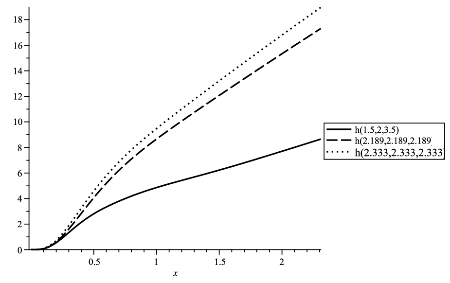
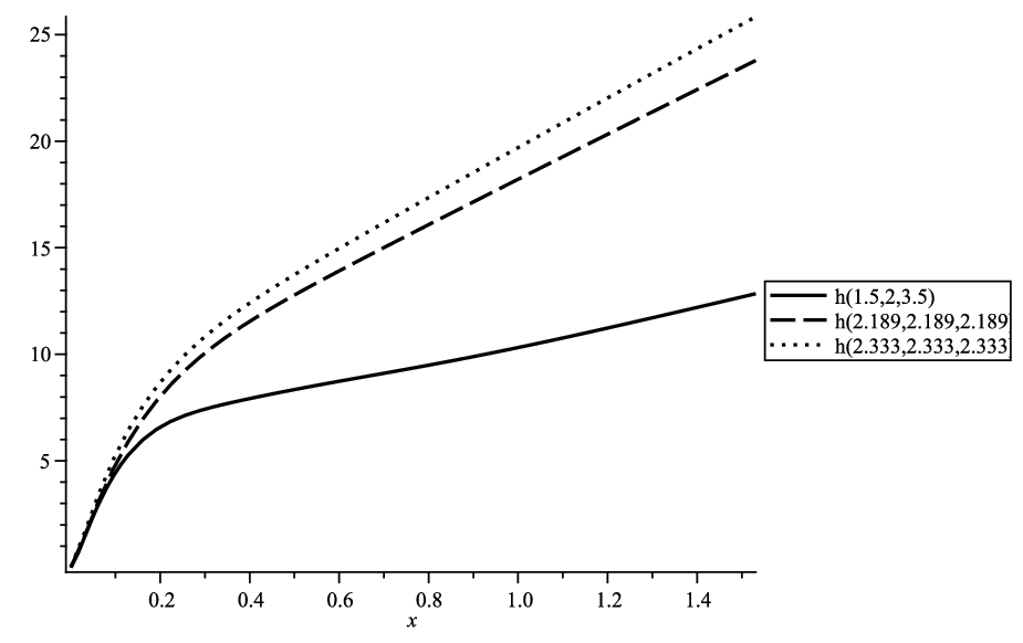
Suppose X1,X2,X3X_{1},X_{2},X_{3} are independent random variables with Xi∼P​G​W​(p,q,λi)X_{i}\sim PGW(p,q,\lambda_{i}), i=1,2,3,i=1,2,3, where (λ1,λ2,λ3)=(1.5,2,3.5)(\lambda_{1},\lambda_{2},\lambda_{3})=(1.5,2,3.5). Further, suppose Y1,Y2,Y3Y_{1},Y_{2},Y_{3} is another set of independent random variables with Yi∼P​G​W​(p,q,λ)Y_{i}\sim PGW(p,q,\lambda), i=1,2,3.i=1,2,3. Assume that the hazard rates of X3:3X_{3:3} and Y3:3Y_{3:3} are denoted, respectively, by h(.;1.5,2,3.5)h(.;1.5,2,3.5) and h(.;λ,λ,λ)h(.;\lambda,\lambda,\lambda). Fig.1 and Fig.2 represent the hazard rate functions of X3:3X_{3:3} and Y3:3Y_{3:3} for the case (p,q)=(1.5,0.8)(p,q)=(1.5,0.8) and (p,q)=(0.8,0.4)(p,q)=(0.8,0.4), respectively, when parameter λ\lambda is taken as λ¯=2.333\bar{\lambda}=2.333 (the arithmetic mean of λi\lambda_{i}’s) and λ~=2.189\tilde{\lambda}=2.189 (the geometric means of λi\lambda_{i}’s). It appears from these figures that the hazard rate function of Y3:3Y_{3:3} in terms of the geometric mean of λi\lambda_{i}’s provides an upper bound for the hazard rate function of X3:3X_{3:3} which is sharper than those in terms of the arithmetic mean of λi\lambda_{i}’s. □\qquad\square

Refer to caption
Figure 1: Plot of the hazard rate functions for p=1.5p=1.5 and q=0.8q=0.8
Refer to caption
Figure 2: Plot of the hazard rate functions for p=0.8p=0.8 and q=0.4q=0.4

4 Comparisons in multiple-outlier model

It is natural to ask whether the result of Theorem 3.1 can be extended to the general case when the lifetimes of two parallel systems are heterogeneous and the vectors of scale parameters are ordered with respect to the pp-larger order. The following example provides a negative answer to this problem.

Example 4.1.

Suppose X1,X2,X3X_{1},X_{2},X_{3} are independent random variables with Xi∼P​G​W​(2,1,λi)X_{i}\sim PGW(2,1,\lambda_{i}), i=1,2,3i=1,2,3, where (λ1,λ2,λ3)=(0.1,1,9)(\lambda_{1},\lambda_{2},\lambda_{3})=(0.1,1,9). Further, suppose Y1,Y2,Y3Y_{1},Y_{2},Y_{3} is another set of independent random variables with Yi∼P​G​W​(2,1,μi)Y_{i}\sim PGW(2,1,\mu_{i}), i=1,2,3i=1,2,3, where (μ1,μ2,μ3)=(0.1,4,6)(\mu_{1},\mu_{2},\mu_{3})=(0.1,4,6). It is easy to observe that (λ1,λ2,λ3)⪰p(μ1,μ2,μ3)(\lambda_{1},\lambda_{2},\lambda_{3})\stackrel{{\scriptstyle p}}{{\succeq}}(\mu_{1},\mu_{2},\mu_{3}). On the other hand, we have

F¯X3:3(0.8)F¯Y3:3(0.8)=1.00339,F¯X3:3(1)F¯Y3:3(1)=1.0037,F¯X3:3(1.9)F¯Y3:3(1.9)=1.0019.\displaystyle\frac{\displaystyle\bar{F}_{X_{3:3}}(0.8)}{\displaystyle\bar{F}_{Y_{3:3}}(0.8)}=1.00339,\qquad\frac{\displaystyle\bar{F}_{X_{3:3}}(1)}{\displaystyle\bar{F}_{Y_{3:3}}(1)}=1.0037,\qquad\frac{\displaystyle\bar{F}_{X_{3:3}}(1.9)}{\displaystyle\bar{F}_{Y_{3:3}}(1.9)}=1.0019.

Thus, the ratio F¯X3:3(x)F¯X3:3(x)\frac{\displaystyle\bar{F}_{X_{3:3}}(x)}{\displaystyle\bar{F}_{X_{3:3}}(x)} is not monotone in x∈ℝ+x\in\mathbb{R^{+}}, which means that X3:3X_{3:3} and Y3:3Y_{3:3} can not be compared with respect to the hazard rate order. □\qquad\square

Since Theorem 3.1 could not be extended to the general case, in the first step attention moves to the multiple-outlier scale model which reduces the complete heterogenity of the scale parameters. In the sequel, we consider parallel systems with the lifetimes of their components following the multiple-outlier scale model and investigate the problem of stochastic comparisons between these systems.

Let us now recall some results in the literature that are most pertinent to the main results that are established in the sequel. Let Z1,⋯,ZnZ_{1},\cdots,Z_{n} be independent exponential random variables with hazard rates λ1,⋯,λn\lambda_{1},\cdots,\lambda_{n}, respectively. Further, let Z1∗,⋯,Zn∗Z^{*}_{1},\cdots,Z^{*}_{n} be another set of independent exponential random variables with hazard rates λ1∗,⋯,λn∗\lambda^{*}_{1},\cdots,\lambda^{*}_{n}, respectively. Then, [pledger1971comparisons] proved that

(λ1,⋯,λn)⪰m(λ1∗,⋯,λn∗)⟹Zk:n≥s​tZk:n∗.\displaystyle(\lambda_{1},\cdots,\lambda_{n})\stackrel{{\scriptstyle m}}{{\succeq}}(\lambda^{*}_{1},\cdots,\lambda^{*}_{n})\Longrightarrow Z_{k:n}\geq_{st}Z^{*}_{k:n}. (4.5)

In the special case of k=2k=2 and n=2n=2, Boland et al. (1994) strengthened (4.5) from the usual stochastic order to the hazard rate order. Moreover, they showed, by means of a counterexample, that (3.10) cannot be extended to the hazard rate order for n≥3n\geq 3. Recently, Zhao and Balakrishnan (2012) improved (3.10) from the usual stochastic order to the hazard rate order for parallel systems in multiple-outlier exponential models. Specifically, let Y1,⋯,YnY_{1},\cdots,Y_{n} be independent exponential random variables with Y1,⋯,YpY_{1},\cdots,Y_{p} having common hazard rate λ1\lambda_{1} and Yp+1,⋯,YnY_{p+1},\cdots,Y_{n} having common hazard rate λ2\lambda_{2}. Further, let Y1∗,⋯,Yn∗Y^{*}_{1},\cdots,Y^{*}_{n} be another set of independent exponential random variables with Y1∗,⋯,Yp∗Y^{*}_{1},\cdots,Y^{*}_{p} having common hazard rate λ1∗\lambda^{*}_{1} and Yp+1∗,⋯,Yn∗Y^{*}_{p+1},\cdots,Y^{*}_{n} having common hazard rate λ2∗\lambda^{*}_{2}. Then, for λ1≤λ1∗≤λ2∗≤λ2\lambda_{1}\leq\lambda^{*}_{1}\leq\lambda^{*}_{2}\leq\lambda_{2}, Zhao and Balakrishnan (2012) showed that

(λ1,⋯,λ1⏟p,λ2,⋯,λ2⏟n−p)⪰p(λ1∗,⋯,λ1∗⏟p,λ2∗,⋯,λ2∗⏟n−p)⟺Yn:n≥h​rYn:n∗⟺Yn:n≥s​tYn:n∗.\displaystyle(\underbrace{\lambda_{1},\cdots,\lambda_{1}}_{p},\underbrace{\lambda_{2},\cdots,\lambda_{2}}_{n-p})\stackrel{{\scriptstyle p}}{{\succeq}}(\underbrace{\lambda^{*}_{1},\cdots,\lambda^{*}_{1}}_{p},\underbrace{\lambda^{*}_{2},\cdots,\lambda^{*}_{2}}_{n-p})\Longleftrightarrow Y_{n:n}\geq_{hr}Y^{*}_{n:n}\Longleftrightarrow Y_{n:n}\geq_{st}Y^{*}_{n:n}. (4.6)

Balakrishnan and Zhao (2013a) and Balakrishnan et al. (2014) extended a result similar to the one in (3.11) for multiple-outlier gamma model and multiple-outlier GE model, respectively.

From Lemma 2.3, Lemma 3.1 and Lemma 3.2 , we obtain a result similar to the one in (3.11) for multiple-outlier PGW model and multiple-outlier GG model.

Theorem 4.1.

Let (X1,1,⋯,X1,n1,X2,1,⋯,X2,n2)(X_{1,1},\cdots,X_{1,n_{1}},X_{2,1},\cdots,X_{2,n_{2}}) and (Y1,1,⋯,Y1,n1,Y2,1,⋯,Y2,n2)(Y_{1,1},\cdots,Y_{1,n_{1}},Y_{2,1},\cdots,Y_{2,n_{2}}) be two independent random vectors with

  • (i)

    Xi,j∼P​G​W​(p,q,λi)X_{i,j}\sim PGW(p,q,\lambda_{i}) and Yi,j∼P​G​W​(p,q,λi∗)Y_{i,j}\sim PGW(p,q,{\lambda}_{i}^{*}), j=1,⋯,nij=1,\cdots,n_{i}, i=1,2i=1,2 or

  • (ii)

    Xi,j∼G​G​(α,q​α,λi)X_{i,j}\sim GG(\alpha,q\alpha,\lambda_{i}) and Yi,j∼G​G​(α,q​α,λi∗)Y_{i,j}\sim GG(\alpha,q\alpha,{\lambda}_{i}^{*}), j=1,⋯,nij=1,\cdots,n_{i}, i=1,2i=1,2.

Assume that λ1≤λ1∗≤λ2∗≤λ2\lambda_{1}\leq\lambda^{*}_{1}\leq\lambda^{*}_{2}\leq\lambda_{2}. Then, for q≤1q\leq 1, the following three statements are equivalent:

  • (i)

    (λ1,⋯,λ1⏟n1,λ2,⋯,λ2⏟n2)⪰p(λ1∗,⋯,λ1∗⏟n1,λ2∗,⋯,λ2∗⏟n2)(\underbrace{\lambda_{1},\cdots,\lambda_{1}}_{n_{1}},\underbrace{\lambda_{2},\cdots,\lambda_{2}}_{n_{2}})\stackrel{{\scriptstyle p}}{{\succeq}}(\underbrace{\lambda^{*}_{1},\cdots,\lambda^{*}_{1}}_{n_{1}},\underbrace{\lambda^{*}_{2},\cdots,\lambda^{*}_{2}}_{n_{2}});

  • (ii)

    Xn:n≥h​rYn:nX_{n:n}\geq_{hr}Y_{n:n};

  • (iii)

    Xn:n≥s​tYn:nX_{n:n}\geq_{st}Y_{n:n}.

Appendix

Suppose r~\tilde{r} denotes the reversed hazard rate function corresponding to FF. Then, from the assumption in C-1, we easily observe that

y​r~​(y)\displaystyle y\tilde{r}(y) =\displaystyle= y​f​(y)∫0yf⁡(u)​𝑑u\displaystyle\frac{\displaystyle yf(y)}{\displaystyle\int_{0}^{y}f(u)du} (4.7)
=\displaystyle= w⁡(y)​h​(y)∫01w⁡(y​u)​h​(y​u)​𝑑u\displaystyle\frac{\displaystyle w(y)h(y)}{\displaystyle\int_{0}^{1}\,w(yu)\,h(yu)du}
=\displaystyle= h⁡(y)∫01w⁡(u)​h​(y​u)​𝑑u.\displaystyle\frac{\displaystyle h(y)}{\displaystyle\int_{0}^{1}w(u)\,h(yu)du}.

Taking derivative from both sides of (4.7), we obtain

(y​r~​(y))′=h′​(y)​∫01w⁡(u)​h​(y​u)​𝑑u−h⁡(y)​∫01u​w​(u)​h′​(y​u)​𝑑u(∫01w⁡(u)​h​(y​u)​𝑑u)2.\displaystyle\Big(y\tilde{r}(y)\Big)^{\prime}=\frac{\displaystyle h^{\prime}(y)\int_{0}^{1}\,w(u)h(yu)\,du-h(y)\int_{0}^{1}u\,w(u)\,h^{\prime}(yu)\,du}{\displaystyle\Big(\int_{0}^{1}\,w(u)\,h(yu)\,du\Big)^{2}}. (4.8)

Moreover, by using the integration by parts and the results in Remark 2-1, we can easily observe that

∫01u​w​(u)​h′​(y​u)​𝑑u=1y​(h⁡(y)−(1+w′​(1))​∫01w⁡(x)​h​(y​u)​𝑑u).\displaystyle\int_{0}^{1}u\,w(u)\,h^{\prime}(yu)\,du=\frac{\displaystyle 1}{\displaystyle y}\,\Big(h(y)-(1+w^{\prime}(1))\int_{0}^{1}w(x)\,h(yu)\,du\Big).

Now, from (4.7) and by substituting the above observation in (4.8), we have

(y​r~​(y))′\displaystyle\Big(y\tilde{r}(y)\Big)^{\prime} =\displaystyle= h′​(y)∫01w⁡(u)​h​(y​u)​𝑑u−h2​(y)y​(∫01w⁡(u)​h​(y​u)​𝑑u)2+(1+w′​(1))​h​(y)y​∫01w⁡(u)​h​(y​u)​𝑑u\displaystyle\frac{\displaystyle h^{\prime}(y)}{\displaystyle\int_{0}^{1}\,w(u)\,h(yu)\,du}-\frac{\displaystyle h^{2}(y)}{\displaystyle y\Big(\int_{0}^{1}\,w(u)\,h(yu)du\Big)^{2}}+\frac{\displaystyle\Big(1+w^{\prime}(1)\Big)h(y)}{\displaystyle y\int_{0}^{1}\,w(u)\,h(yu)du} (4.9)
=\displaystyle= (y​r~​(y))​h′​(y)h⁡(y)−y​r~2​(y)+(1+w′​(1))​r~​(y).\displaystyle\Big(y\tilde{r}(y)\Big)\,\frac{\displaystyle h^{\prime}(y)}{\displaystyle h(y)}-y\tilde{r}^{2}(y)+\Big(1+w^{\prime}(1)\Big)\tilde{r}(y).
Lemma 4.1.

Consider the decomposition form in (2.3) under the assumptions C-1 and C-2. Suppose the following hold:

  • (aa)

    x​(r~​(x)−h′​(x)h⁡(x))x\,(\tilde{r}(x)-\frac{h^{\prime}(x)}{h(x)}) is increasing in x∈ℝ+x\in\mathbb{R}^{+};

  • (bb)

    F¯​(x)≤−w⁡(x)​h2​(x)h′​(x)\bar{F}(x)\leq-\frac{w(x)\,h^{2}(x)}{h^{\prime}(x)} for every x∈ℝ+x\in\mathbb{R}^{+}.

Then,

  • (i)

    1+w′​(1)>01+w^{\prime}(1)>0,

  • (ii)

    for αi≥1,i=1,⋯,n\alpha_{i}\geq 1,\,\,i=1,\cdots,n, we have

    ∑i=1nαi​yi​r~​(yi)−yp​(r~​(yp)−h′​(yp)h⁡(yp))​(1−∏i=1n(F⁡(yi))αi)≥0,\displaystyle\sum_{i=1}^{n}\,\alpha_{i}y_{i}\tilde{r}(y_{i})-y_{p}\Big(\tilde{r}(y_{p})-\frac{\displaystyle h^{\prime}(y_{p})}{\displaystyle h(y_{p})}\Big)\,\Big(1-\prod_{i=1}^{n}\,\big(F(y_{i})\big)^{\alpha_{i}}\Big)\geq 0, (4.10)

    where yi∈ℝ+y_{i}\in\mathbb{R}^{+}, i=1,⋯,ni=1,\cdots,n, and yp=min⁡(y1,⋯,yn)y_{p}=\min(y_{1},\cdots,y_{n}). Further, for the special case of n=1n=1, the result in (4.10) holds just under the assumption (bb).

Proof  

  • (i)

    If h⁡(x)h(x) is increasing, then the assumption (b) in not hold. So we assume that h⁡(x)h(x) is decreasing in xx and we have;

    1\displaystyle 1 =\displaystyle= ∫0∞xw′​(1)​h​(x)​𝑑x\displaystyle\int_{0}^{\infty}x^{w^{\prime}(1)}h(x)dx
    =\displaystyle= ∫01xw′​(1)​h​(x)​𝑑x+∫1∞xw′​(1)​h​(x)​𝑑x\displaystyle\int_{0}^{1}x^{w^{\prime}(1)}h(x)dx+\int_{1}^{\infty}x^{w^{\prime}(1)}h(x)dx
    ≥\displaystyle\geq ∫01xw′​(1)​h​(x)​𝑑x\displaystyle\int_{0}^{1}x^{w^{\prime}(1)}h(x)dx
    ≥\displaystyle\geq min0<x<1⁡(h⁡(x))​∫01xw′​(1)​𝑑x\displaystyle\min_{0<x<1}(h(x))\int_{0}^{1}x^{w^{\prime}(1)}dx
    =\displaystyle= h⁡(1)​(1w′​(1)+1−limx⟶0x1+w′​(1)1+w′​(1))⟹1+w′​(1)>0\displaystyle h(1)\bigg(\frac{1}{w^{\prime}(1)+1}-\lim_{x\longrightarrow 0}\frac{x^{1+w^{\prime}(1)}}{1+w^{\prime}(1)}\bigg)\Longrightarrow 1+w^{\prime}(1)>0
  • (ii)

    From the assumptions (bb) and 𝐂−𝟏{\bf C-1}, and the decomposition form in (2.3) we have

    F⁡(yi)F¯​(yi)\displaystyle\frac{F(y_{i})}{\displaystyle\bar{F}(y_{i})} ≥\displaystyle\geq −h′​(yi)w⁡(yi)​h2​(yi)∫01yiw(yiu)h(yiu)du\displaystyle-\frac{\displaystyle h^{\prime}(y_{i})}{\displaystyle w(y_{i})\,h^{2}(y_{i})}\,\int_{0}^{1}y_{i}\,w(y_{i}u)\,h(y_{i}u)\,du
    =\displaystyle= −yih′​(yi)h2​(yi)∫01w(u)h(yiu)du,i=1,⋯,n,\displaystyle-y_{i}\,\frac{\displaystyle h^{\prime}(y_{i})}{\displaystyle h^{2}(y_{i})}\,\int_{0}^{1}w(u)\,h(y_{i}u)\,du,\qquad\quad i=1,\cdots,n,

    which, according to (4.7), implies

    F¯​(yi)\displaystyle\bar{F}(y_{i}) ≤\displaystyle\leq 11−(yi​h′​(yi)h2​(yi))​∫01w⁡(u)​h​(yi​u)​𝑑u\displaystyle\frac{\displaystyle 1}{\displaystyle 1-\Big(y_{i}\,\frac{\displaystyle h^{\prime}(y_{i})}{\displaystyle h^{2}(y_{i})}\Big)\int_{0}^{1}w(u)\,h(y_{i}u)\,du} (4.11)
    =\displaystyle= h⁡(yi)∫01w⁡(u)​h​(yi​u)​𝑑uh⁡(yi)∫01w⁡(u)​h​(yi​u)​𝑑u−yi​h′​(yi)h⁡(yi)\displaystyle\frac{\displaystyle\frac{\displaystyle h(y_{i})}{\displaystyle\int_{0}^{1}w(u)\,h(y_{i}u)\,du}}{\frac{\displaystyle h(y_{i})}{\displaystyle\int_{0}^{1}\,w(u)\,h(y_{i}u)\,du}-y_{i}\,\frac{\displaystyle h^{\prime}(y_{i})}{\displaystyle h(y_{i})}}
    =\displaystyle= r~​(yi)r~​(yi)−h′​(yi)h⁡(yi),i=1,⋯,n.\displaystyle\frac{\displaystyle\tilde{r}(y_{i})}{\displaystyle\tilde{r}(y_{i})-\frac{\displaystyle h^{\prime}(y_{i})}{\displaystyle h(y_{i})}},\qquad\quad i=1,\cdots,n.

Now, from Proposition 2 of [balakrishnan and zhao 2013] and (4.11), we obtain

1−∏i=1n(F⁡(yi))αi\displaystyle 1-\prod_{i=1}^{n}\big(F(y_{i})\big)^{\alpha_{i}} ≤\displaystyle\leq ∑i=1n1−(F⁡(yi))αi\displaystyle\sum_{i=1}^{n}1-\big({F}(y_{i})\big)^{\alpha_{i}} (4.12)
≤\displaystyle\leq ∑i=1nαi​(1−F⁡(yi))\displaystyle\sum_{i=1}^{n}{\alpha_{i}}\big(1-{F}(y_{i})\big)
≤\displaystyle\leq ∑i=1nαi​r~​(yi)r~​(yi)−h′​(yi)h⁡(yi).\displaystyle\sum_{i=1}^{n}\alpha_{i}\frac{\displaystyle\tilde{r}(y_{i})}{\displaystyle\tilde{r}(y_{i})-\frac{\displaystyle h^{\prime}(y_{i})}{\displaystyle h(y_{i})}}.

Note that, for the special case of n=1n=1, (4.12) coincides with (4.11) which holds just under the assumption (bb). Now, let us assume that n>1n>1. For i=1,⋯,ni=1,\cdots,n, set

γi=yi​r~​(yi)h⁡(yi),βi=r~​(yi)h⁡(yi)r~​(yi)−h′​(yi)h⁡(yi),δi=αi​h​(yi).\gamma_{i}=\frac{\displaystyle y_{i}\,\tilde{r}(y_{i})}{\displaystyle h(y_{i})},\qquad\beta_{i}=\frac{\displaystyle\frac{\displaystyle\tilde{r}(y_{i})}{\displaystyle h(y_{i})}}{\displaystyle\tilde{r}(y_{i})-\frac{\displaystyle h^{\prime}(y_{i})}{\displaystyle h(y_{i})}},\quad\delta_{i}=\alpha_{i}h(y_{i}).

So, from Proposition 1 of [balakrishnan and zhao 2013], it follows that

∑i=1nαi​yi​r~​(yi)∑i=1nαi​r~​(yi)r~​(yi)−h′​(yi)h⁡(yi)\displaystyle\frac{\displaystyle\sum_{i=1}^{n}\alpha_{i}y_{i}\tilde{r}(y_{i})}{\displaystyle\sum_{i=1}^{n}\alpha_{i}\frac{\displaystyle\tilde{r}(y_{i})}{\displaystyle\tilde{r}(y_{i})-\frac{\displaystyle h^{\prime}(y_{i})}{\displaystyle h(y_{i})}}} ≥\displaystyle\geq min1≤i≤n⁡{γiβi}\displaystyle\min_{1\leq i\leq n}\,\Bigg\{\frac{\displaystyle\gamma_{i}}{\displaystyle\beta_{i}}\Bigg\} (4.13)
=\displaystyle= yp​(r~​(yp)−h′​(yp)h⁡(yp)),\displaystyle y_{p}\Big(\tilde{r}(y_{p})-\frac{\displaystyle h^{\prime}(y_{p})}{\displaystyle h(y_{p})}\Big),

where the last equality is obtained from the assumption (aa). Now, based on (4.12) and (4.13), we get

∑i=1nαi​yi​r~​(yi)1−∏i=1n(F⁡(yi))αi\displaystyle\frac{\displaystyle\sum_{i=1}^{n}\alpha_{i}y_{i}\tilde{r}(y_{i})}{\displaystyle 1-\prod_{i=1}^{n}\big(F(y_{i})\big)^{\alpha_{i}}} ≥\displaystyle\geq ∑i=1nαi​yi​r~​(yi)∑i=1nαi​r~​(yi)r~​(yi)−h′​(yi)h⁡(yi)\displaystyle\frac{\displaystyle\sum_{i=1}^{n}\alpha_{i}y_{i}\tilde{r}(y_{i})}{\displaystyle\sum_{i=1}^{n}\alpha_{i}\frac{\displaystyle\tilde{r}(y_{i})}{\displaystyle\tilde{r}(y_{i})-\frac{\displaystyle h^{\prime}(y_{i})}{\displaystyle h(y_{i})}}}
≥\displaystyle\geq yp​(r~​(yp)−h′​(yp)h⁡(yp)),\displaystyle y_{p}\Big(\tilde{r}(y_{p})-\frac{\displaystyle h^{\prime}(y_{p})}{\displaystyle h(y_{p})}\Big),

which completes the proof of the lemma.□\qquad\square

Lemma 4.2.

Suppose X1,⋯,XnX_{1},\cdots,X_{n} are independent non-negative random variables with Xi∼F⁡(λ​x)X_{i}\sim F(\lambda x), i=1,⋯,pi=1,\cdots,p, and Xj∼F⁡(λ∗​x)X_{j}\sim F(\lambda^{*}x), j=p+1,⋯,n,j=p+1,\cdots,n, where λ≤λ∗\lambda\leq\lambda^{*}. Further, suppose the following assumptions hold:

  • (aa)

    x​(r~​(x)−h′​(x)h⁡(x))x\,(\tilde{r}(x)-\frac{h^{\prime}(x)}{h(x)}) is increasing in x∈ℝ+x\in\mathbb{R}^{+};

  • (bb)

    F¯​(x)≤−w⁡(x)​h2​(x)h′​(x)\bar{F}(x)\leq-\frac{w(x)\,h^{2}(x)}{h^{\prime}(x)} for every x∈ℝ+x\in\mathbb{R}^{+}.

Then, the hazard rate function of Xn:nX_{n:n} is increasing in λ∈(0,λ∗].\lambda\in(0,\lambda^{*}].

Proof  The hazard rate function of Xn:nX_{n:n} can be expressed as

rXn:n(x)\displaystyle r_{X_{n:n}}(x) =\displaystyle= (Fp​(λ​x)​Fn−p​(λ∗​x)1−Fp​(λ​x)​Fn−p​(λ∗​x))​(p​λ​r~​(λ​x)+(n−p)​λ∗​r~​(λ∗​x))\displaystyle\Bigg(\frac{F^{p}(\lambda x)F^{n-p}(\lambda^{*}x)}{1-F^{p}(\lambda x)F^{n-p}(\lambda^{*}x)}\Bigg)\Big(p\lambda\tilde{r}(\lambda x)+(n-p)\lambda^{*}\tilde{r}(\lambda^{*}x)\Big)
=\displaystyle= 1x​φ​(λ​x,λ∗​x),x>0,\displaystyle\frac{\displaystyle 1}{\displaystyle x}\varphi(\lambda x,\lambda^{*}x),\qquad x>0,

where the continuously differentiable function ϕ:ℝ+2→ℝ+\phi:\mathbb{R^{+}}^{2}\rightarrow\mathbb{R^{+}} is defined as

φ⁡(y,y∗)=(Fp​(y)​Fn−p​(y∗)1−Fp​(y)​Fn−p​(y∗))​(p​y​r~​(y)+(n−p)​y∗​r~​(y∗)),y≤y∗.\displaystyle\varphi(y,y^{*})=\Bigg(\frac{F^{p}(y)F^{n-p}(y^{*})}{1-F^{p}(y)F^{n-p}(y^{*})}\Bigg)\Big(py\tilde{r}(y)+(n-p)y^{*}\tilde{r}(y^{*})\Big),\quad y\leq y^{*}. (4.14)

In order to prove the required result, it suffices to show that φ⁡(y,y∗)\varphi(y,y^{*}) is increasing in y∈(0,y∗]y\in(0,y^{*}]. The partial derivative of φ⁡(y,y∗)\varphi(y,y^{*}) with respect to yy is

∂φ⁡(y,y∗)∂y=p⁡(Fp​(y)​Fn−p​(y∗)(1−Fp​(y)​Fn−p​(y∗))2)​(r~​(y)​(p​y1​r~​(y)+(n−p)​y∗​r~​(y∗))+(y​r~​(y))′​(1−Fp​(y)​Fn−p​(y∗))),\displaystyle\frac{\displaystyle\partial\varphi(y,y^{*})}{\displaystyle\partial y}=p\Bigg(\frac{F^{p}(y)F^{n-p}(y^{*})}{\Big(1-F^{p}(y)F^{n-p}(y^{*})\Big)^{2}}\Bigg)\Bigg(\tilde{r}(y)\Big(py_{1}\tilde{r}(y)+(n-p)y^{*}\tilde{r}(y^{*})\Big)+\Big(y\tilde{r}(y)\Big)^{\prime}\,\Big(1-F^{p}(y)F^{n-p}(y^{*})\Big)\Bigg),

which, based on (4.9), becomes

∂φ⁡(y,y∗)∂y\displaystyle\frac{\displaystyle\partial\varphi(y,y^{*})}{\displaystyle\partial y} =\displaystyle= p(Fp​(y)​Fn−p​(y∗)(1−Fp​(y)​Fn−p​(y∗))2){(1+w′(1))(1−Fp(y)Fn−p(y∗))r~(y)\displaystyle p\Bigg(\frac{F^{p}(y)F^{n-p}(y^{*})}{\Big(1-F^{p}(y)F^{n-p}(y^{*})\Big)^{2}}\Bigg)\Bigg\{\Big(1+w^{\prime}(1)\Big)\Big(1-F^{p}(y)F^{n-p}(y^{*})\Big)\tilde{r}(y) (4.15)
+r~(y)(pyr~(y)+(n−p)y∗r~(y∗)−y(r~(y)−h′​(y)h⁡(y))(1−Fp(y)Fn−p(y∗)))}.\displaystyle\quad+\tilde{r}(y)\,\Bigg(py\tilde{r}(y)+(n-p)y^{*}\tilde{r}(y^{*})-y\Big(\tilde{r}(y)-\frac{\displaystyle h^{\prime}(y)}{\displaystyle h(y)}\Big)\Big(1-F^{p}(y)F^{n-p}(y^{*})\Big)\Bigg)\Bigg\}.

Now, from the part (i) of Lemma 4.1, we observe that the first term on the right hand side of (4.15) is non-negative. On the other hand, since y≤y∗y\leq y^{*}, then from the assumption (a)(a) and (b)(b) and Lemma 4.1, it follows that the second term on the right hand side of (4.15) is also non-negative. This completes the proof of the lemma. □\qquad\square

Lemma 4.3.

Suppose X1,⋯,XnX_{1},\cdots,X_{n} are independent non-negative random variables with common distribution function (F⁡(λ​x))α\big(F(\lambda x)\big)^{\alpha}. Further, suppose the following hold:

F¯​(x)≤−w⁡(x)​h2​(x)h′​(x)\bar{F}(x)\leq-\frac{w(x)\,h^{2}(x)}{h^{\prime}(x)} for every x∈ℝ+x\in\mathbb{R}^{+}.

Then, for α≥1\alpha\geq 1 the hazard rate function of Xn:nX_{n:n} is increasing in λ∈ℝ+\lambda\in\mathbb{R}^{+}.

Proof  Suppose Y1,⋯,YnY_{1},\cdots,Y_{n} are independent non-negative random variables with common distribution function (F⁡(μ​x))αi\big(F(\mu x)\big)^{\alpha_{i}} where λ≤μ\lambda\leq\mu. In order to prove the required result, it suffices to show that Xn:n≥h​rYn:nX_{n:n}\geq_{hr}Y_{n:n}. To this end, in view of Theorem 1.B.36 of Shaked and Shanthikumar (2007), it is enough to show that Xi≥h​rYiX_{i}\geq_{hr}Y_{i} for i=1,⋯,ni=1,\cdots,n. Setting p=n=1p=n=1 in (4.14), we observe that the hazard rate function of XiX_{i} is rXi​(x)=1x​φ​(λ​x),r_{X_{i}}(x)=\frac{1}{x}\,\varphi(\lambda x),. Now, to derive the result that Xi≥h​rYiX_{i}\geq_{hr}Y_{i}, we need to show that φ\varphi is increasing in y∈ℝ+y\in\mathbb{R}^{+}. From (4.15), we have

φ′​(y)=α​(F⁡(y))α(1−(F⁡(y))α)2​{(1+w′​(1))​(F⁡(y))α​r~​(y)+r~​(y)​(α​y​r~​(y)−y⁡(r~​(y)−y​h′​(y)h⁡(y))​(1−(F⁡(y))α))}.\displaystyle\varphi^{\prime}(y)=\alpha\frac{\displaystyle\big(F(y)\big)^{\alpha}}{\displaystyle\Big(1-\big(F(y)\big)^{\alpha}\Big)^{2}}\Bigg\{\Big(1+w^{\prime}(1)\Big)\big(F(y)\big)^{\alpha}\tilde{r}(y)+\tilde{r}(y)\Bigg(\alpha y\tilde{r}(y)-y\Big(\tilde{r}(y)-y\frac{\displaystyle h^{\prime}(y)}{h(y)}\Big)\Big(1-\big(F(y)\big)^{\alpha}\Big)\Bigg)\Bigg\}. (4.16)

according to Lemma 4.1, φ′\varphi^{\prime} is non-negative and the proof is thus completed. □\qquad\square
The following lemma plays a vital role in the sequel.

Lemma 4.4.

For n>1n>1, let ϕ:ℝ+2​n⟶ℝ+\phi:\mathbb{R}_{+}^{2n}\longrightarrow\mathbb{R}_{+} be a continuously differentiable mapping. If the following assumptions hold:

  • (a)

    (λi−λj)​(λiαi​∂ϕ⁡(α,λ)∂λi−λjαj​∂ϕ⁡(α,λ)∂λj)≥0(\lambda_{i}-\lambda_{j})\big(\frac{\lambda_{i}}{\alpha_{i}}\frac{\partial\phi(\alpha,\lambda)}{\partial\lambda_{i}}-\frac{\lambda_{j}}{\alpha_{j}}\frac{\partial\phi(\alpha,\lambda)}{\partial\lambda_{j}}\big)\geq 0,

  • (b)

    1αi​∂ϕ⁡(α,λ)∂λi|λi=z=1αj​∂ϕ⁡(α,λ)∂λj|λj=z\frac{1}{\alpha_{i}}\frac{\partial\phi(\alpha,\lambda)}{\partial\lambda_{i}}|_{\lambda_{i}=z}=\frac{1}{\alpha_{j}}\frac{\partial\phi(\alpha,\lambda)}{\partial\lambda_{j}}|_{\lambda_{j}=z},

Then, for any 𝕩=(x1,⋯,xn)∈(0,∞)n\mathbb{x}=(x_{1},\cdots,x_{n})\in(0,\infty)^{n}, the following inequality holds:

ϕ⁡(α,𝕩)≥ϕ⁡(α,𝕩~).\displaystyle\phi(\alpha,\mathbb{x})\geq\phi(\alpha,\mathbb{\tilde{x}}). (4.17)

Where, α=(α1,⋯,αn)\alpha=(\alpha_{1},\cdots,\alpha_{n}), 𝕩~=(x~,⋯,x~)\mathbb{\tilde{x}}=(\tilde{x},\cdots,\tilde{x}) and x~=∏i=1nxiαi∑i=1nαi\tilde{x}=\prod_{i=1}^{n}x_{i}^{\frac{\alpha_{i}}{\sum_{i=1}^{n}\alpha_{i}}}.

Proof For a fixed vector 𝕩=(x1,⋯,xn)∈(0,∞)n\mathbb{x}=(x_{1},\cdots,x_{n})\in(0,\infty)^{n} let consider a=min⁡xia=\min{x_{i}}, b=max⁡xib=\max{x_{i}}, 𝕩~=(x~,⋯,x~)\tilde{\mathbb{x}}=(\tilde{x},\cdots,\tilde{x}). Inequality (4.17) is an equality for a=ba=b.
Let us assume a<ba<b. Then x~∈(a,b)\tilde{x}\in(a,b). We consider the compact subset KK of (0,∞)n(0,\infty)^{n}:

K={𝕥=(t1,⋯,tn)∈[a,b]n|∏i=1ntiαi∑i=1nαi=x~}K=\big\{\mathbb{t}=(t_{1},\cdots,t_{n})\in[a,b]^{n}|\prod_{i=1}^{n}t_{i}^{\frac{\alpha_{i}}{\sum_{i=1}^{n}\alpha_{i}}}=\tilde{x}\big\}

Clearly, 𝕩\mathbb{x} and 𝕩~\tilde{\mathbb{x}} belong to K. From Weierstrass’s theorem it follows that the continuous mapping ϕ\phi reaches an absolute minimum on the compact KK on some point 𝕦=(u1,…,un)∈K\mathbb{u}=(u_{1},...,u_{n})\in K.
Now let us assume 𝕦≠𝕩~\mathbb{u}\neq\tilde{\mathbb{x}}. In this case, there exists p,q∈{1,2,⋯,n}p,q\in\{1,2,\cdots,n\} such that a≤up=min⁡ui<max⁡ui≤ba\leq u_{p}=\min{u_{i}}<\max{u_{i}}\leq b. Now we have,

upαp​uqαq​∏i≠p,qnuiαi=mu_{p}^{{\alpha_{p}}}u_{q}^{{\alpha_{q}}}\prod_{i\neq p,q}^{n}u_{i}^{{\alpha_{i}}}=m

Where m=x~∑i=1nαim=\tilde{x}^{\sum_{i=1}^{n}\alpha_{i}}. The equation zαp+αq​∏i≠p,qnuiαi=mz^{{\alpha_{p}}+{\alpha_{q}}}\prod_{i\neq p,q}^{n}u_{i}^{{\alpha_{i}}}=m has a positive solution in zz which is denoted z1z_{1}. Clearly,

z1αp+αq=upαp​uqαq,up<z1<uq\displaystyle z_{1}^{{\alpha_{p}}+{\alpha_{q}}}=u_{p}^{{\alpha_{p}}}u_{q}^{{\alpha_{q}}},\qquad\qquad u_{p}<z_{1}<u_{q} (4.18)

For t∈[up,z​1)t\in[u_{p},z1), let us consider the function g⁡(t)g(t) defined on [up,z​1)[u_{p},z1) by the relation:

gαq​(t)=upαp​uqαqtαp∈(z1,uq],∀t∈[up,z​1)g^{{\alpha_{q}}}(t)=\frac{u_{p}^{{\alpha_{p}}}u_{q}^{{\alpha_{q}}}}{t^{{\alpha_{p}}}}\in(z_{1},u_{q}],\qquad\forall t\in[u_{p},z1)

The continuously differentiable decreasing function g has the following derivative:

g′​(t)=−αp​upαp​uqαqαq​gαq−1​(t)​tαp+1\displaystyle g^{\prime}(t)=-\frac{\alpha_{p}u_{p}^{{\alpha_{p}}}u_{q}^{{\alpha_{q}}}}{\alpha_{q}g^{\alpha_{q}-1}(t)\,t^{\alpha_{p}+1}} (4.19)

Let 𝕦⁡(t)=(u1​(t),u2​(t),⋯,un​(t))\mathbb{u}(t)=(u_{1}(t),u_{2}(t),\cdots,u_{n}(t)), where up​(t)=t,uq​(t)=g⁡(t)u_{p}(t)=t,\,\,u_{q}(t)=g(t) and ui​(t)=uiu_{i}(t)=u_{i} when i≠p,qi\neq p,q. Now let us consider the continuously differentiable function ψ:[up,z1)⟶ℝ\psi:[u_{p},z_{1})\longrightarrow\mathbb{R}, ψ⁡(t)=ϕ⁡(α,𝕦⁡(t))\psi(t)=\phi(\alpha,\mathbb{u}(t)). The derivative of ψ⁡(t)\psi(t) with respect to tt, is

ψ′​(t)\displaystyle\psi^{\prime}(t) =\displaystyle= ∂ϕ⁡(α,𝕦⁡(t))∂up​(t)​∂up​(t)∂t+∂ϕ⁡(α,𝕦⁡(t))∂uq​(t)​∂uq​(t)∂t\displaystyle\frac{\partial\phi(\alpha,\mathbb{u}(t))}{\partial u_{p}(t)}\frac{\partial u_{p}(t)}{\partial t}+\frac{\partial\phi(\alpha,\mathbb{u}(t))}{\partial u_{q}(t)}\frac{\partial u_{q}(t)}{\partial t}
=\displaystyle= ∂ϕ⁡(α,𝕦⁡(t))∂up​(t)+∂ϕ⁡(α,𝕦⁡(t))∂uq​(t)​g′​(t)\displaystyle\frac{\partial\phi(\alpha,\mathbb{u}(t))}{\partial u_{p}(t)}+\frac{\partial\phi(\alpha,\mathbb{u}(t))}{\partial u_{q}(t)}g^{\prime}(t)

Let t=upt=u_{p}, then g⁡(up)=uqg(u_{p})=u_{q}. So

ψ′​(up)\displaystyle\psi^{\prime}(u_{p}) =\displaystyle= ∂ϕ⁡(α,𝕦⁡(t))∂up​(t)|t=up−αp​uqαq​up​∂ϕ⁡(α,𝕦⁡(t))∂uq​(t)|t=up\displaystyle\frac{\partial\phi(\alpha,\mathbb{u}(t))}{\partial u_{p}(t)}|_{t=u_{p}}-\frac{\alpha_{p}u_{q}}{\alpha_{q}u_{p}}\frac{\partial\phi(\alpha,\mathbb{u}(t))}{\partial u_{q}(t)}|_{t=u_{p}}
=\displaystyle= αpup​[upαp​∂ϕ⁡(α,𝕦⁡(t))∂up​(t)|t=up−uqαq​∂ϕ⁡(α,𝕦⁡(t))∂uq​(t)|t=up]\displaystyle\frac{\alpha_{p}}{u_{p}}\big[\frac{u_{p}}{\alpha_{p}}\frac{\partial\phi(\alpha,\mathbb{u}(t))}{\partial u_{p}(t)}|_{t=u_{p}}-\frac{u_{q}}{\alpha_{q}}\frac{\partial\phi(\alpha,\mathbb{u}(t))}{\partial u_{q}(t)}|_{t=u_{p}}\big]

But, from assumptions (a) and (b), it follows that ψ′​(z)=0\psi^{\prime}(z)=0 and for up<zu_{p}<z, ψ′​(up)<0\psi^{\prime}(u_{p})<0. Hence, there exists ε>0\varepsilon>0 such that up+ε<zu_{p}+\varepsilon<z and ψ′​(t)<0\psi^{\prime}(t)<0, ∀∈[up,up+ε)\forall\in[u_{p},u_{p}+\varepsilon). Therefore, ϕ⁡(𝕦⁡(t))<ϕ⁡(𝕦⁡(up))=ϕ⁡(𝕦)\phi(\mathbb{u}(t))<\phi(\mathbb{u}(u_{p}))=\phi(\mathbb{u}), for any t∈(up,up+ε)t\in(u_{p},u_{p}+\varepsilon). This gives the contradiction. Then the unique minimum point of ϕ\phi on K is 𝕦\mathbb{u} and the relation (4.17) follows. □\qquad\square
Proof of lemma 2.1
(i)
⇒\Rightarrow (ii). The hazard rate function of Xn:nX_{n:n} can be rewritten as

rXn:n(x)\displaystyle r_{X_{n:n}}(x) =\displaystyle= (∏i=1n(F⁡(λi​x))αi1−∏i=1n(F⁡(λi​x))αi)​∑i=1nαi​λi​r~​(λi​x)\displaystyle\Bigg(\frac{\displaystyle\prod_{i=1}^{n}\big(F(\lambda_{i}x)\big)^{\alpha_{i}}}{\displaystyle 1-\prod_{i=1}^{n}\big(F(\lambda_{i}x)\big)^{\alpha_{i}}}\Bigg)\,\sum_{i=1}^{n}\alpha_{i}\lambda_{i}\tilde{r}(\lambda_{i}x)
=\displaystyle= 1x​ψ​(λ1​x,⋯,λn​x),x>0,\displaystyle\frac{\displaystyle 1}{\displaystyle x}\,\psi(\lambda_{1}x,\cdots,\lambda_{n}x),\qquad x>0,

where r~​(x)=f​(x)/F​(x)\tilde{r}(x)={f(x)}/{F(x)} and the symmetric and continuously differentiable function ψ:ℝ+n→ℝ+\psi:\,{\mathbb{R}^{+}}^{n}\rightarrow\,{\mathbb{R}^{+}} is defined as

ψ⁡(y1,⋯,yn)=(∏i=1n(F⁡(yi))αi1−∏i=1n(F⁡(yi))αi)​∑i=1nαi​yi​r~​(yi).\displaystyle\psi(y_{1},\cdots,y_{n})=\Bigg(\frac{\displaystyle\prod_{i=1}^{n}\big(F(y_{i})\big)^{\alpha_{i}}}{\displaystyle 1-\prod_{i=1}^{n}\big(F(y_{i})\big)^{\alpha_{i}}}\Bigg)\,\sum_{i=1}^{n}\alpha_{i}y_{i}\tilde{r}(y_{i}). (4.20)

Similarly, the hazard rate function of Yn:nY_{n:n} can be expressed as

rYn:n(x)=1xψ(λx,⋯,λx),x>0.\displaystyle r_{Y_{n:n}}(x)=\frac{\displaystyle 1}{\displaystyle x}\,\psi(\lambda x,\cdots,\lambda x),\qquad x>0.

First, we show that ψ⁡(y1,⋯,yn)≤ψ⁡(y~,⋯,y~⏟n)\psi(y_{1},\cdots,y_{n})\leq\psi(\underbrace{\tilde{y},\cdots,\tilde{y}}_{n}), where λ~=∏i=1nλiαi∑i=1nαi\tilde{\lambda}=\prod_{i=1}^{n}\lambda_{i}^{\frac{\alpha_{i}}{\sum_{i=1}^{n}\alpha_{i}}}. To this end, we will utilize Lemma 4.4 Set yp=min⁡(y1,⋯,yn)y_{p}=\min(y_{1},\cdots,y_{n}) and yq=max⁡(y1,⋯,yn)y_{q}=\max(y_{1},\cdots,y_{n}). Then, we have

∂ψ⁡(𝐲)∂yp=αp​(∏i=1n(F⁡(yi))αi(1−∏i=1n(F⁡(yi))αi)2)​(r~​(yp)​∑i=1nαi​yi​r~​(yi)+(yp​r~​(yp))′​(1−∏i=1n(F⁡(yi))αi)),\displaystyle\frac{\displaystyle\partial\psi({\bf y})}{\displaystyle\partial y_{p}}=\alpha_{p}\Bigg(\frac{\displaystyle\prod_{i=1}^{n}\big(F(y_{i})\big)^{\alpha_{i}}}{\displaystyle\Big(1-\prod_{i=1}^{n}\big(F(y_{i})\big)^{\alpha_{i}}\Big)^{2}}\Bigg)\Bigg(\tilde{r}(y_{p})\sum_{i=1}^{n}\alpha_{i}y_{i}\tilde{r}(y_{i})+\Big(y_{p}\tilde{r}(y_{p})\Big)^{\prime}\Big(1-\prod_{i=1}^{n}\big(F(y_{i})\big)^{\alpha_{i}}\Big)\Bigg),

which, according to (4.9), converts to

∂ψ⁡(𝐲)∂yp\displaystyle\frac{\displaystyle\partial\psi({\bf y})}{\displaystyle\partial y_{p}} =\displaystyle= αp(∏i=1n(F⁡(yi))αi(1−∏i=1n(F⁡(yi))αi)2){(1+w′(1))(1−∏i=1n(F(yi))αi)r~(yp)\displaystyle\alpha_{p}\Bigg(\frac{\displaystyle\prod_{i=1}^{n}\big(F(y_{i})\big)^{\alpha_{i}}}{\displaystyle\Big(1-\prod_{i=1}^{n}\big(F(y_{i})\big)^{\alpha_{i}}\Big)^{2}}\Bigg)\Bigg\{\Big(1+w^{\prime}(1)\Big)\Big(1-\prod_{i=1}^{n}\big(F(y_{i})\big)^{\alpha_{i}}\Big)\tilde{r}(y_{p})
+r~(yp)(∑i=1nαiyir~(yi)−yp(r~(yp)−yph′​(yp)h⁡(yp))(1−∏i=1n(F(yi))αi))}.\displaystyle\qquad\qquad\qquad\qquad\quad+\tilde{r}(y_{p})\Bigg(\sum_{i=1}^{n}\,\alpha_{i}y_{i}\tilde{r}(y_{i})-y_{p}\Big(\tilde{r}(y_{p})-y_{p}\frac{\displaystyle h^{\prime}(y_{p})}{h(y_{p})}\Big)\Big(1-\prod_{i=1}^{n}\big(F(y_{i})\big)^{\alpha_{i}}\Big)\Bigg)\Bigg\}.

Since the function ψ\psi is symmetric, then each partial derivative of it has the same structure. Thus, we have

∂ψ⁡(𝐲)∂yp\displaystyle\frac{\displaystyle\partial\psi({\bf y})}{\displaystyle\partial y_{p}} =\displaystyle= αq(∏i=1n(F⁡(yi))αi(1−∏i=1n(F⁡(yi))αi)2){(1+w′(1))(1−∏i=1n(F(yi))αi)r~(yq)\displaystyle\alpha_{q}\Bigg(\frac{\displaystyle\prod_{i=1}^{n}\big(F(y_{i})\big)^{\alpha_{i}}}{\displaystyle\Big(1-\prod_{i=1}^{n}\big(F(y_{i})\big)^{\alpha_{i}}\Big)^{2}}\Bigg)\Bigg\{\Big(1+w^{\prime}(1)\Big)\Big(1-\prod_{i=1}^{n}\big(F(y_{i})\big)^{\alpha_{i}}\Big)\tilde{r}(y_{q})
+r~(yq)(∑i=1nαiyir~(yi)−yq(r~(yq)−yqh′​(yq)h⁡(yq))(1−∏i=1n(F(yi))αi))}.\displaystyle\qquad\qquad\qquad\qquad\quad+\tilde{r}(y_{q})\Bigg(\sum_{i=1}^{n}\,\alpha_{i}y_{i}\tilde{r}(y_{i})-y_{q}\Big(\tilde{r}(y_{q})-y_{q}\frac{\displaystyle h^{\prime}(y_{q})}{h(y_{q})}\Big)\Big(1-\prod_{i=1}^{n}\big(F(y_{i})\big)^{\alpha_{i}}\Big)\Bigg)\Bigg\}.

Now, based on the above derivatives, we get

ypαp​∂ψ⁡(𝒚)∂yp−yqαq​∂ψ⁡(𝒚)∂yq\displaystyle\frac{y_{p}}{\alpha_{p}}\frac{\displaystyle\partial\psi(\mbox{\boldmath$y$})}{\partial y_{p}}-\frac{y_{q}}{\alpha_{q}}\frac{\displaystyle\partial\psi(\mbox{\boldmath$y$})}{\partial y_{q}} =s​g​n\displaystyle\stackrel{{\scriptstyle sgn}}{{=}} (1+ω′​(1))​(yp​r~​(yp)−yq​r~​(yq))​(1−∏i=1n(F⁡(yi))αi)\displaystyle\Big(1+\omega^{\prime}(1)\Big)\Bigg(y_{p}\tilde{r}(y_{p})-y_{q}\tilde{r}(y_{q})\Bigg)\Big(1-\prod_{i=1}^{n}\big(F(y_{i})\big)^{\alpha_{i}}\Big) (4.21)
+yp​r~​(yp)​(∑i=1nαi​yi​r~​(yi)−yp​(r~​(yp)−h′​(yp)h⁡(yp))​(1−∏i=1n(F⁡(yi))αi))\displaystyle\,\,\,+y_{p}\tilde{r}(y_{p})\Bigg(\sum_{i=1}^{n}\,\alpha_{i}y_{i}\tilde{r}(y_{i})-y_{p}\Big(\tilde{r}(y_{p})-\frac{h^{\prime}(y_{p})}{h(y_{p})}\Big)\Big(1-\prod_{i=1}^{n}\big(F(y_{i})\big)^{\alpha_{i}}\Big)\Bigg)
−yq​r~​(yq)​(∑i=1nαi​yi​r~​(yi)−yq​(r~​(yq)−h′​(yq)h⁡(yq))​(1−∏i=1n(F⁡(yi))αi))\displaystyle\qquad-y_{q}\tilde{r}(y_{q})\Bigg(\sum_{i=1}^{n}\,\alpha_{i}y_{i}\tilde{r}(y_{i})-y_{q}\Big(\tilde{r}(y_{q})-\frac{h^{\prime}(y_{q})}{h(y_{q})}\Big)\Big(1-\prod_{i=1}^{n}\big(F(y_{i})\big)^{\alpha_{i}}\Big)\Bigg)
=\displaystyle= A1+A2,\displaystyle A_{1}+A_{2},

where a=s​g​nba\stackrel{{\scriptstyle sgn}}{{=}}b means that aa and bb have the same sign and

A1=(1+ω′​(1))​(yp​r~​(yp)−yq​r~​(yq))​(1−∏i=1n(F⁡(yi))αi)A_{1}=\Big(1+\omega^{\prime}(1)\Big)\Bigg(y_{p}\tilde{r}(y_{p})-y_{q}\tilde{r}(y_{q})\Bigg)\Big(1-\prod_{i=1}^{n}\big(F(y_{i})\big)^{\alpha_{i}}\Big)

and

A2=yp​r~​(yp)​(∑i=1nαi​yi​r~​(yi)−yp​(r~​(yp)−h′​(yp)h⁡(yp))​(1−∏i=1n(F⁡(yi))αi))−yq​r~​(yq)​(∑i=1nαi​yi​r~​(yi)−yq​(r~​(yq)−h′​(yq)h⁡(yq))​(1−∏i=1n(F⁡(yi))αi)).A_{2}=y_{p}\tilde{r}(y_{p})\Bigg(\sum_{i=1}^{n}\,\alpha_{i}y_{i}\tilde{r}(y_{i})-y_{p}\Big(\tilde{r}(y_{p})-\frac{h^{\prime}(y_{p})}{h(y_{p})}\Big)\Big(1-\prod_{i=1}^{n}\big(F(y_{i})\big)^{\alpha_{i}}\Big)\Bigg)-y_{q}\tilde{r}(y_{q})\Bigg(\sum_{i=1}^{n}\,\alpha_{i}y_{i}\tilde{r}(y_{i})-y_{q}\Big(\tilde{r}(y_{q})-\frac{h^{\prime}(y_{q})}{h(y_{q})}\Big)\Big(1-\prod_{i=1}^{n}\big(F(y_{i})\big)^{\alpha_{i}}\Big)\Bigg).

From the part (i) of Lemma 4.1 and assumptions (b)(b), it readily follows that A1≥0A_{1}\geq 0. On the other hand, for αi≥1,i=1,⋯,n\alpha_{i}\geq 1,\,\,i=1,\cdots,n we have

A2\displaystyle A_{2} ≥\displaystyle\geq yq​r~​(yq)​(1−∏i=1n(F⁡(yi))αi)​(yq​(r~​(yq)−h′​(yq)h⁡(yq))−yp​(r~​(yp)−h′​(yp)h⁡(yp)))\displaystyle y_{q}\tilde{r}(y_{q})\Big(1-\prod_{i=1}^{n}\big(F(y_{i})\big)^{\alpha_{i}}\Big)\Bigg(y_{q}\Big(\tilde{r}(y_{q})-\frac{h^{\prime}(y_{q})}{h(y_{q})}\Big)-y_{p}\Big(\tilde{r}(y_{p})-\frac{h^{\prime}(y_{p})}{h(y_{p})}\Big)\Bigg)
≥\displaystyle\geq 0,\displaystyle 0,

where the first inequality obtains from the assumptions (a)(a), (b)(b), (c)(c) and Lemma 4.1, while the second inequality follows from the assumption (bb). Also, it is easy to see that

1αp​∂ψ⁡(𝒚)∂yp|yp=z−1αq​∂ψ⁡(𝒚)∂yq|yp=z=0\displaystyle\frac{1}{\alpha_{p}}\frac{\displaystyle\partial\psi(\mbox{\boldmath$y$})}{\partial y_{p}}|_{y_{p}=z}-\frac{1}{\alpha_{q}}\frac{\displaystyle\partial\psi(\mbox{\boldmath$y$})}{\partial y_{q}}|_{y_{p}=z}=0 (4.22)

Therefore, from Lemma 4.4, (4.21) and (4.22), it follows that ψ⁡(λ1​x,⋯,λn​x)≤ψ⁡(λ~​x,⋯,λ~​x)\psi(\lambda_{1}x,\cdots,\lambda_{n}x)\leq\psi(\tilde{\lambda}x,\cdots,\tilde{\lambda}x). On the other hand, from the part (i) of Lemma 4.1 and assumption (cc), and Lemma 2.5 it follows that the hazard rate function of Yn:nY_{n:n} is increasing in λ∈ℝ+\lambda\in\mathbb{R}^{+}, that is, ψ⁡(λ~​x,⋯,λ~​x)≤ψ⁡(λ​x,⋯,λ​x)\psi(\tilde{\lambda}x,\cdots,\tilde{\lambda}x)\leq\psi(\lambda x,\cdots,\lambda x) for λ≥λ~\lambda\geq\tilde{\lambda}. By combining these observations, (ii) follows.

(ii) ⇒\Rightarrow (iii). It is clear since the hazard rate order implies the usual stochastic order.

(iii) ⇒\Rightarrow (i). From the statement (iii), we have FXn:n(x)FYn:n(x)≤1\frac{F_{X_{n:n}}(x)}{F_{Y_{n:n}}(x)}\leq 1 for every x>0x>0. Thus,

∏i=1n(l​i​mx→0​F⁡(λi​x)F⁡(λ​x))αi\displaystyle\prod_{i=1}^{n}\left(lim_{x\rightarrow 0}\frac{F(\lambda_{i}x)}{F(\lambda x)}\right)^{\alpha_{i}} =\displaystyle= l​i​mx→0​∏i=1n(F⁡(λi​x)F⁡(λ​x))αi\displaystyle lim_{x\rightarrow 0}\,\prod_{i=1}^{n}\,\,\left(\frac{F(\lambda_{i}x)}{F(\lambda x)}\right)^{\alpha_{i}} (4.23)
≤\displaystyle\leq 1.\displaystyle 1.

On the other hand, according to the L’Hopital’s rule, and Remark 2.1, and assumption C-2, we obtain

l​i​mx→0​F⁡(λi​x)F⁡(λ​x)\displaystyle lim_{x\rightarrow 0}\frac{F(\lambda_{i}x)}{F(\lambda x)} =\displaystyle= l​i​mx→0​λi​f​(λi​x)λ​f​(λ​x)\displaystyle lim_{x\rightarrow 0}\frac{\lambda_{i}\,f(\lambda_{i}x)}{\lambda\,f(\lambda x)} (4.24)
=\displaystyle= (λiλ)1+w′​(1)​l​i​mx→0​h⁡(λi​x)h⁡(λ​x)\displaystyle\Big(\frac{\lambda_{i}}{\lambda}\Big)^{1+w^{\prime}(1)}\,\,lim_{x\rightarrow 0}\frac{h(\lambda_{i}x)}{h(\lambda x)}
=\displaystyle= (λiλ)(1+w′​(1)).\displaystyle(\frac{\lambda_{i}}{\lambda})^{(1+w^{\prime}(1))}.

Hence, by substituting (4.24) into (4.23) and using the part (i) of Lemma 4.1, we have λ≥λ~\lambda\geq\tilde{\lambda} which completes the proof of the theorem. □\qquad\square

The following known result provides an approach for testing whether a vector valued function is Schur-convex (Schur-concave) or not.

Lemma 4.5.

(Marshall et al. 2011, p. 84) Suppose I⊂ℝI\subset\mathbb{R} is an open interval and suppose ϕ:In→ℝ\phi\,:\,I^{n}\rightarrow\mathbb{R} is continuously differentiable. Necessary and sufficient conditions for ϕ\phi to be Schur-convex (Schur-concave) on InI^{n} are the symmetric property of ϕ\phi on InI^{n}, and

(xi−xj)​(∂ϕ∂xi​(𝐱)−∂ϕ∂xj​(𝐱))≥(≤)​0,f​o​r​a​l​l​i≠j​a​n​d​𝐱=(x1,⋯,xn)∈In,\displaystyle(x_{i}-x_{j})\left(\frac{\partial\phi}{\partial x_{i}}({\bf x})-\frac{\partial\phi}{\partial x_{j}}({\bf x})\right)\,\geq(\leq)0,\qquad\,for\,\,all\,\,i\not=j\,\,and\,\,{\bf x}=(x_{1},\cdots,x_{n})\in I^{n},

where ∂ϕ∂xi​(𝐱)\frac{\partial\phi}{\partial x_{i}}({\bf x}) denotes the partial derivative of ϕ\phi with respect to its ii-th argument.

Proof of lemma 2.2  Set a=log⁡λa=\log\lambda and a∗=log⁡λ∗a^{*}=\log\lambda^{*}. Then, the hazard rate function of Xn:nX_{n:n}, in terms of aa and a∗a^{*}, is given by

rXn:n(x;a,a∗)=1xϕ(x​ea,⋯,x​ea⏟p,x​ea∗,⋯,x​ea∗⏟n−p),\displaystyle r_{X_{n:n}}(x;a,a^{*})=\frac{\displaystyle 1}{\displaystyle x}\,\phi(\underbrace{xe^{a},\cdots,xe^{a}}_{p},\underbrace{xe^{a^{*}},\cdots,xe^{a^{*}}}_{n-p}),

where

ϕ⁡(y,⋯,y⏟p,y∗,⋯,y∗⏟n−p)=(Fp​(y)​Fn−p​(y∗)1−Fp​(y)​Fn−p​(y∗))​(p​y​r~​(y)+(n−p)​y∗​r~​(y∗)).\displaystyle\phi(\underbrace{y,\cdots,y}_{p},\underbrace{y^{*},\cdots,y^{*}}_{n-p})=\Bigg(\frac{F^{p}(y)F^{n-p}(y^{*})}{1-F^{p}(y)F^{n-p}(y^{*})}\Bigg)\Big(py\tilde{r}(y)+(n-p)y^{*}\tilde{r}(y^{*})\Big).

For simplicity in presentation, we denote ϕ⁡(y,⋯,y⏟p,y∗,⋯,y∗⏟n−p)\phi(\underbrace{y,\cdots,y}_{p},\underbrace{y^{*},\cdots,y^{*}}_{n-p}) by ϕ⁡(y,y∗)\phi(y,y^{*}). In order to prove the desired result, in the light of Lemma 4.5, it suffices to show that for fixed x>0x>0,

(a−a∗)​(∂ϕ⁡(x​ea,x​ea∗)∂a−∂ψ⁡(x​ea,x​ea∗)∂a∗)≤0.\displaystyle(a-a^{*})\Bigg(\frac{\displaystyle\partial\phi(xe^{a},xe^{a^{*}})}{\displaystyle\partial a}-\frac{\displaystyle\partial\psi(xe^{a},xe^{a^{*}})}{\displaystyle\partial a^{*}}\Bigg)\leq 0. (4.25)

Note that

∂ϕ⁡(x​ea,x​ea∗)∂a\displaystyle\frac{\displaystyle\partial\phi(xe^{a},xe^{a^{*}})}{\partial a} =\displaystyle= ∂(x​ea)∂a​∂ϕ⁡(x​ea,x​ea∗)​∂(x​ea)\displaystyle\frac{\displaystyle\partial\Big(xe^{a}\Big)}{\displaystyle\partial a}\,\,{\displaystyle\partial\phi(xe^{a},xe^{a^{*}})}{\displaystyle\partial\Big(xe^{a}\Big)}
=\displaystyle= x​ea​∂ϕ⁡(x​ea,x​ea∗)∂(x​ea).\displaystyle xe^{a}\,\,\frac{\displaystyle\partial\phi(xe^{a},xe^{a^{*}})}{\displaystyle\partial\Big(xe^{a}\Big)}.

Similarly,

∂ϕ⁡(x​ea,x​ea∗)∂a∗=x​ea∗​∂ϕ⁡(x​ea,x​ea∗)∂(x​ea∗).\displaystyle\frac{\displaystyle\partial\phi(xe^{a},xe^{a^{*}})}{\partial a^{*}}=xe^{a^{*}}\,\,\frac{\displaystyle\partial\phi(xe^{a},xe^{a^{*}})}{\displaystyle\partial\Big(xe^{a^{*}}\Big)}.

Now, using these observations, we get

∂ϕ⁡(x​ea,x​ea∗)∂a−∂ϕ⁡(x​ea,x​ea∗)∂a∗=\displaystyle\frac{\displaystyle\partial\phi(xe^{a},xe^{a^{*}})}{\displaystyle\partial a}-\frac{\displaystyle\partial\phi(xe^{a},xe^{a^{*}})}{\displaystyle\partial a^{*}}= x​ea​∂ϕ⁡(x​ea,x​ea∗)∂(x​ea)−x​ea∗​∂ϕ⁡(x​ea,x​ea∗)∂(x​ea∗).\displaystyle xe^{a}\,\,\frac{\displaystyle\partial\phi(xe^{a},xe^{a^{*}})}{\displaystyle\partial\Big(xe^{a}\Big)}-xe^{a^{*}}\,\,\frac{\displaystyle\partial\phi(xe^{a},xe^{a^{*}})}{\displaystyle\partial\Big(xe^{a^{*}}\Big)}. (4.26)

So, from (4.26), we easily observe that (4.25) satisfies if we could show that

(ln⁡y−ln⁡y∗)​(y​∂ψ⁡(y,y∗)∂y−y∗​∂ψ⁡(y,y∗)∂y∗)≤0.\displaystyle(\ln y-\ln y^{*})\Bigg(y\,\frac{\displaystyle\partial\psi(y,y^{*})}{\displaystyle\partial y}-y^{*}\,\frac{\displaystyle\partial\psi(y,y^{*})}{\displaystyle\partial y^{*}}\Bigg)\leq 0. (4.27)

To this end, we have

y​∂ϕ⁡(y,y∗)∂y−y∗​∂ψ⁡(y,y∗)∂y∗\displaystyle y\frac{\displaystyle\partial\phi(y,y^{*})}{\displaystyle\partial y}-y^{*}\frac{\displaystyle\partial\psi(y,y^{*})}{\displaystyle\partial y^{*}} =s​g​n\displaystyle\stackrel{{\scriptstyle sgn}}{{=}} (1+ω′​(1))​(y​r~​(y)−y∗​r~​(y∗))​(1−Fp​(y)​Fn−p​(y∗))\displaystyle(1+\omega^{\prime}(1))\Big(y\tilde{r}(y)-y^{*}\tilde{r}(y^{*})\Big)\Big(1-F^{p}(y)F^{n-p}(y^{*})\Big) (4.28)
+y​r~​(y)​((p​y​r~​(y)+(n−p)​y∗​r~​(y∗))−y⁡(r~​(y)−h′​(y)h⁡(y))​(1−Fp​(y)​Fn−p​(y∗)))\displaystyle\,\,\,+y\tilde{r}(y)\Bigg(\Big(p\,y\tilde{r}(y)+(n-p)\,y^{*}\tilde{r}(y^{*})\Big)-y\Big(\tilde{r}(y)-\frac{h^{\prime}(y)}{h(y)}\Big)\Big(1-F^{p}(y)F^{n-p}(y^{*})\Big)\Bigg)
−y∗​r~​(y∗)​((p​y​r~​(y)+(n−p)​y∗​r~​(y∗))−y∗​(r~​(y∗)−h′​(y∗)h⁡(y∗))​(1−Fp​(y)​Fn−p​(y∗)))\displaystyle\quad-y^{*}\tilde{r}(y^{*})\Bigg(\Big(p\,y\tilde{r}(y)+(n-p)\,y^{*}\tilde{r}(y^{*})\Big)-y^{*}\Big(\tilde{r}(y^{*})-\frac{h^{\prime}(y^{*})}{h(y^{*})}\Big)\Big(1-F^{p}(y)F^{n-p}(y^{*})\Big)\Bigg)
=\displaystyle= B1+B2,\displaystyle B_{1}+B_{2},

where

B1=(1+ω′​(1))​(1−Fp​(y)​Fn−p​(y∗))​(y​r~​(y)−y∗​r~​(y∗)),\displaystyle B_{1}=(1+\omega^{\prime}(1))\Big(1-F^{p}(y)F^{n-p}(y^{*})\Big)\Big(y\tilde{r}(y)-y^{*}\tilde{r}(y^{*})\Big),
B2\displaystyle B_{2} =\displaystyle= y​r~​(y)​((p​y​r~​(y)+(n−p)​y∗​r~​(y∗))−y⁡(r~​(y)−h′​(y)h⁡(y))​(1−Fp​(y)​Fn−p​(y∗)))\displaystyle y\tilde{r}(y)\Bigg(\Big(p\,y\tilde{r}(y)+(n-p)\,y^{*}\tilde{r}(y^{*})\Big)-y\Big(\tilde{r}(y)-\frac{h^{\prime}(y)}{h(y)}\Big)\Big(1-F^{p}(y)F^{n-p}(y^{*})\Big)\Bigg)
−y∗​r~​(y∗)​((p​y​r~​(y)+(n−p)​y∗​r~​(y∗))−y∗​(r~​(y∗)−h′​(y∗)h⁡(y∗))​(1−Fp​(y)​Fn−p​(y∗))).\displaystyle\quad-y^{*}\tilde{r}(y^{*})\Bigg(\Big(p\,y\tilde{r}(y)+(n-p)\,y^{*}\tilde{r}(y^{*})\Big)-y^{*}\Big(\tilde{r}(y^{*})-\frac{h^{\prime}(y^{*})}{h(y^{*})}\Big)\Big(1-F^{p}(y)F^{n-p}(y^{*})\Big)\Bigg).

Let us first assume that y∗≥yy^{*}\geq y. Then, from assumptions (bb) and the part (i) of Lemma 4.1, we can easily observe that B1≥0B_{1}\geq 0. Furthermore, according to assumptions (a)(a), (b)(b), (cc) and Lemma 4.1, it follows that

B2\displaystyle B_{2} ≥\displaystyle\geq y∗​r~​(y∗)​(1−Fp​(y)​Fn−p​(y∗))​(y∗​(r~​(y∗)−h′​(y∗)h⁡(y∗))−y⁡(r~​(y)−h′​(y)h⁡(y)))\displaystyle y^{*}\tilde{r}(y^{*})\Big(1-F^{p}(y)F^{n-p}(y^{*})\Big)\Bigg(y^{*}\Big(\tilde{r}(y^{*})-\frac{h^{\prime}(y^{*})}{h(y^{*})}\Big)-y\Big(\tilde{r}(y)-\frac{h^{\prime}(y)}{h(y)}\Big)\Bigg)
≥\displaystyle\geq 0.\displaystyle 0.

These observations result that (4.28) is non-negative. For the case when y>y∗y>y^{*}, by using an argument similar to the above, one can easily show that B1≤0B_{1}\leq 0 and B2≤0B_{2}\leq 0, i.e, (4.28) is non-positive. Consequently, (4.27) is satisfied and the proof is thus completed. □\qquad\square
Proof of lemma 2.3  Suppose (i) holds. Then, (ii) immediately follows from Lemma 2.2 for the case when λp​λ∗n−p=μp​μ∗n−p\lambda^{p}{\lambda^{*}}^{n-p}=\mu^{p}{\mu^{*}}^{n-p}. Now, let us assume that λp​λ∗n−p<μp​μ∗n−p\lambda^{p}{\lambda^{*}}^{n-p}<\mu^{p}{\mu^{*}}^{n-p}. Setting λ0=μ​(μ∗λ∗)(n−p)/p\lambda_{0}=\mu\,(\frac{\mu^{*}}{\lambda^{*}})^{(n-p)/p}, then it can be easily seen that

λ<λ0≤μ≤μ∗≤λ∗a​n​dλ0p​λ∗n−p=μp​μ∗n−p.\displaystyle\lambda<\lambda_{0}\leq\mu\leq\mu^{*}\leq\lambda^{*}\qquad and\qquad\lambda^{p}_{0}{\lambda^{*}}^{n-p}=\mu^{p}{\mu^{*}}^{n-p}.

Suppose Z1,⋯,ZnZ_{1},\cdots,Z_{n} are independent non-negative random variables with Zi∼F⁡(λ0​x)Z_{i}\sim F(\lambda_{0}x), i=1,⋯,pi=1,\cdots,p, and Zj∼F⁡(λ∗​x)Z_{j}\sim F(\lambda^{*}x), j=p+1,⋯,nj=p+1,\cdots,n. From Lemma 2.2, we have Zn:n≥h​rYn:nZ_{n:n}\geq_{hr}Y_{n:n}. On the other hand, from Lemma 4.2, it follows that Xn:n≥h​rZn:nX_{n:n}\geq_{hr}Z_{n:n}. Now, by combining these results, (ii) follows. Since the hazard rate order implies the usual stochastic order, then (ii) ⇒\Rightarrow (iii). The proof of the implication (iii) ⇒\Rightarrow (i) is similar to that of Lemma 2.1, and therefore omitted here. This completes the proof of the theorem.□\qquad\square

Lemma 4.6.

Let the function ψ(.):ℝ+⟶ℝ+\psi(.):\mathbb{R}^{+}\longrightarrow\mathbb{R}^{+} be defined as

ψ⁡(x)=q⁡(q−1)+ex−1​((q−1)2​x+q​x2−x1+q+2​q​(1−q))\displaystyle\psi(x)=q\,(q-1)+e^{x-1}\bigg((q-1)^{2}x+q\,x^{2}-x^{1+q}+2q(1-q)\bigg)

Then, for each q∈(0,1]q\in(0,1], ψ⁡(x)≥0\psi(x)\geq 0.

Proof. If q=1q=1, we can easily observe that ψ⁡(x)=0\psi(x)=0 for all x∈[0,∞)x\in[0,\infty). Now, let us assume that q<1q<1. After some simplifications, we obtain that

∂∂x​ψ​(x)|x=1\displaystyle\frac{\partial}{\partial x}\psi(x)|_{x=1} =\displaystyle= 0\displaystyle 0
∂2∂x2​ψ​(x)|x=1\displaystyle\frac{\partial^{2}}{\partial x^{2}}\psi(x)|_{x=1} =\displaystyle= 0\displaystyle 0

And

∂3∂x3​ψ​(x)|x=1\displaystyle\frac{\partial^{3}}{\partial x^{3}}\psi(x)|_{x=1} =\displaystyle= −q3−q2+2​q\displaystyle-q^{3}-q^{2}+2q
>\displaystyle> 0∀q∈(0,1).\displaystyle 0\qquad\forall q\in(0,1).

Therefore, ψ′​(x)\psi^{\prime}(x) has a local minimum at x=1x=1 for all q∈(0,1)q\in(0,1). So, there exists some ϵ>0\epsilon>0 such that ψ⁡(x)>ψ⁡(1)\psi(x)>\psi(1) for all x∈(1,1+ϵ)x\in(1,1+\epsilon) and q∈(0,1)q\in(0,1). Also, it is easy to see that

ψ⁡(1)=0a​n​dlimx⟶∞ψ⁡(x)=∞.\displaystyle\psi(1)=0\qquad and\qquad\lim_{x\longrightarrow\infty}\psi(x)=\infty.

Now, suppose minx≥1⁡ψ⁡(x)<0\min_{x\geq 1}\psi(x)<0. Then, From the above observation, ψ⁡(x)\psi(x) has to cross the level 00 at least twice. That is, there exist a point ξ>0\xi>0 such that ψ⁡(ξ)=0\psi(\xi)=0. Then using this in

∂∂x​ψ​(x)=ex−1​((q−1)2​x+q​x2−x1+q+2​q​(1−q))+ex−1​((q−1)2+2​q​x−(1+q)​xq)\displaystyle\frac{\partial}{\partial x}\psi(x)=e^{x-1}\bigg((q-1)^{2}x+q\,x^{2}-x^{1+q}+2q(1-q)\bigg)+e^{x-1}\bigg((q-1)^{2}+2\,q\,x-(1+q)\,x^{q}\bigg)

we obtain that,

∂∂x​ψ​(x)|x=ξ=eξ−1​((q−1)2+2​q​ξ−(1+q)​ξq)−q⁡(q−1).\displaystyle\frac{\partial}{\partial x}\psi(x)|_{x=\xi}=e^{\xi-1}\bigg((q-1)^{2}+2\,q\,\xi-(1+q)\xi^{q}\bigg)-q\,(q-1).

Let,

g⁡(x)=ex−1​((q−1)2+2​q​x−(1+q)​xq)−q⁡(q−1).\displaystyle g(x)=e^{x-1}\bigg((q-1)^{2}+2\,q\,x-(1+q)x^{q}\bigg)-q\,(q-1).

Now, we need to show that g⁡(x)≥0g(x)\geq 0 for all x∈[1,∞)x\in[1,\infty). It is easy to see that

g⁡(1)=0a​n​dlimx⟶∞g⁡(x)=∞..\displaystyle g(1)=0\qquad and\qquad\lim_{x\longrightarrow\infty}g(x)=\infty..

Suppose minx>1⁡g⁡(x)<0\min_{x>1}g(x)<0. The derivative of g⁡(x)g(x) with respect to xx, is

g′​(x)=ex−1​((q−1)2+2​q​x−(1+q)​xq)+ex−1​(2​q−q⁡(1+q)​xq−1),.\displaystyle g^{\prime}(x)=e^{x-1}\bigg((q-1)^{2}+2\,q\,x-(1+q)x^{q}\bigg)+e^{x-1}\bigg(2\,q-q\,(1+q)x^{q-1}\bigg),.

Using the above relations, g′​(1)=2​b2>0g^{\prime}(1)=2\,b^{2}>0. Then g⁡(x)g(x) has to cross the level 00 at least twice, since g⁡(1)=0g(1)=0, g⁡(∞)=∞g(\infty)=\infty, and g′​(1)=2​b2>0g^{\prime}(1)=2\,b^{2}>0. At any point tt that g⁡(t)=0g(t)=0, we have

et−1​((q−1)2+2​q​t−(1+q)​tq)=q⁡(q−1)\displaystyle e^{t-1}\bigg((q-1)^{2}+2\,q\,t-(1+q)t^{q}\bigg)=q\,(q-1)

Using this in g′​(x)g^{\prime}(x),

g′​(x)|x=t=et−1​(2​q−q⁡(1+q)​tq−1)+q⁡(q−1)\displaystyle g^{\prime}(x)|_{x=t}=e^{t-1}\bigg(2\,q-q(1+q)t^{q-1}\bigg)+q\,(q-1)

It is easy to see that g′​(t)>0g^{\prime}(t)>0. Thus, tt is unique. That is a contradiction with g⁡(x)g(x) has to cross the level 00 at least twice. Then ψ′​(ξ)>0\psi^{\prime}(\xi)>0 , since g⁡(x)>0g(x)>0 for all x∈(1,∞)x\in(1,\infty). Thus, ξ\xi is unique. That is a contradiction with ψ⁡(x)\psi(x) has to cross the level 00 at least twice. So, the crossing point ξ\xi does not exist, from which the required result follows. □\qquad\square

Proof of lemma 3.1. As mentioned before, the baseline density function can be written as the decomposition form in (2.3) with

w⁡(x)=xp−1a​n​dh⁡(x)=pq​(1+xp)1q−1​e1−(1+xp)1q,x∈ℝ+,\displaystyle w(x)=x^{p-1}\qquad and\qquad h(x)=\frac{\displaystyle p}{\displaystyle q}(1+x^{p})^{\frac{1}{q}-1}e^{1-(1+x^{p})^{\frac{1}{q}}},\qquad x\in\mathbb{R^{+}},

[khaledi2011stochastic] showed that x​r~​(x)x\tilde{r}(x) is decreasing in x∈ℝ+x\in\mathbb{R^{+}}, and so the assumption (aa) of Lemma 2.1 is satisfied. Now, let us check the assumption (bb). After some algebraic computation, we obtain

s⁡(x)\displaystyle s(x) =\displaystyle= x​(r~​(x)−h′​(x)h⁡(x))\displaystyle x\Big(\tilde{r}(x)-\frac{\displaystyle h^{\prime}(x)}{\displaystyle h(x)}\Big)
=\displaystyle= pq​xp​((1+xp)1q−1​e1−(1+xp)1q1−e1−(1+xp)1q−1−q−(1+xp)1q1+xp)\displaystyle\frac{p}{q}\,x^{p}\bigg(\frac{\displaystyle(1+x^{p})^{\frac{1}{q}-1}\,e^{1-(1+x^{p})^{\frac{1}{q}}}}{\displaystyle 1-e^{1-(1+x^{p})^{\frac{1}{q}}}}-\frac{\displaystyle 1-q-(1+x^{p})^{\frac{1}{q}}}{\displaystyle 1+x^{p}}\bigg)
=\displaystyle= pq​h​(1+xp).\displaystyle\frac{p}{q}h(1+x^{p}).

Where the continuously differentiable h:[1,∞)⟶ℝ+h:[1,\infty)\longrightarrow\mathbb{R}^{+} is defined as

h⁡(x)\displaystyle h(x) =\displaystyle= (x−1)​(x1q−1ex1q−1−1−1−q−x1qx).\displaystyle(x-1)\bigg(\frac{\displaystyle x^{\frac{1}{q}-1}}{\displaystyle e^{x^{\frac{1}{q}}-1}-1}-\frac{\displaystyle 1-q-x^{\frac{1}{q}}}{\displaystyle x}\bigg).

Then, we have

∂s⁡(x)∂x\displaystyle\frac{\partial s(x)}{\partial x} =\displaystyle= ∂(1+xp)∂x​∂s⁡(x)∂(1+xp)\displaystyle\frac{\partial(1+x^{p})}{\partial x}\frac{\partial s(x)}{\partial(1+x^{p})}
=s​g​n\displaystyle\overset{sgn}{=} ∂h⁡(x)∂x\displaystyle\frac{\partial h(x)}{\partial x}
=\displaystyle= x1q−1ex1q−1−1−1−q−x1qx+(x−1)​(x1q−1​(1q−1)x⁡(ex1q−1−1)−x2q−2​ex1q−1q​(ex1q−1−1)2+x1qq​x2+1−q−x1qx2)\displaystyle\frac{\displaystyle x^{\frac{1}{q}-1}}{\displaystyle e^{x^{\frac{1}{q}}-1}-1}-\frac{\displaystyle 1-q-x^{\frac{1}{q}}}{\displaystyle x}+(x-1)\bigg(\frac{\displaystyle x^{\frac{1}{q}-1}(\frac{1}{q}-1)}{\displaystyle x\,\big(e^{x^{\frac{1}{q}}-1}-1\big)}-\frac{\displaystyle x^{\frac{2}{q}-2}\,e^{x^{\frac{1}{q}}-1}}{\displaystyle q\,\big(e^{x^{\frac{1}{q}}-1}-1\big)^{2}}+\frac{\displaystyle x^{\frac{1}{q}}}{\displaystyle q\,x^{2}}+\frac{\displaystyle 1-q-x^{\frac{1}{q}}}{\displaystyle x^{2}}\bigg)
=\displaystyle= 1(ex1q−1−1)2​b​x2​(−q+q2​e2​t1q−2−2​q2​ex1q−1−xq+2q​ex1q−1+q2−xq+1q​ex1q−1−x1q​q​ex1q−1CLOSE\displaystyle\frac{1}{\displaystyle(e^{x^{\frac{1}{q}}-1}-1)^{2}\,b\,x^{2}}\big(-q+q^{2}e^{2t^{\frac{1}{q}}-2}-2\,q^{2}e^{x^{\frac{1}{q}}-1}-x^{\frac{q+2}{q}}e^{x^{\frac{1}{q}}-1}+q^{2}-x^{\frac{q+1}{q}}e^{x^{\frac{1}{q}}-1}-x^{\frac{1}{q}}q\,e^{x^{\frac{1}{q}}-1}
OPEN+x1q​ex1q−1+xq+1q​e2​x1q−2+x1q​q​e2​x1q−2−x1q​e2​x1q−2+2​q​ex1q−1+x2q​ex1q−1−q​e2​x1q−2)\displaystyle+x^{\frac{1}{q}}e^{x^{\frac{1}{q}}-1}+x^{\frac{q+1}{q}}e^{2x^{\frac{1}{q}}-2}+x^{\frac{1}{q}}q\,e^{2x^{\frac{1}{q}}-2}-x^{\frac{1}{q}}e^{2x^{\frac{1}{q}}-2}+2\,q\,e^{x^{\frac{1}{q}}-1}+x^{\frac{2}{q}}e^{x^{\frac{1}{q}}-1}-q\,e^{2x^{\frac{1}{q}}-2}\big)
=s​g​n\displaystyle\overset{sgn}{=} q⁡(q−1)+e2​x1q−2​(q⁡(q−1)+x1+qq+x1q​(q−1))+ex1q−1​(x2q−x1+qq−x2+qq+(1−q)​x1q+2​q​(1−q))\displaystyle q\,(q-1)+e^{2x^{\frac{1}{q}}-2}\big(q(q-1)+x^{\frac{1+q}{q}}+x^{\frac{1}{q}}(q-1)\big)+e^{x^{\frac{1}{q}}-1}\big(x^{\frac{2}{q}}-x^{\frac{1+q}{q}}-x^{\frac{2+q}{q}}+(1-q)x^{\frac{1}{q}}+2\,q\,(1-q)\big)
≥\displaystyle\geq q⁡(q−1)+ex1q−1​(x1q​(q⁡(q−1)+x1+qq+x1q​(q−1))+x2q−x1+qq−x2+qq+(1−q)​x1q+2​q​(1−q))\displaystyle q\,(q-1)+e^{x^{\frac{1}{q}}-1}\bigg(x^{\frac{1}{q}}\big(q(q-1)+x^{\frac{1+q}{q}}+x^{\frac{1}{q}}(q-1)\big)+x^{\frac{2}{q}}-x^{\frac{1+q}{q}}-x^{\frac{2+q}{q}}+(1-q)x^{\frac{1}{q}}+2\,q\,(1-q)\bigg)
=\displaystyle= q⁡(q−1)+ex1q−1​((q−1)2​x1q+q​x2q−x1+qq+2​q​(1−q))\displaystyle q\,(q-1)+e^{x^{\frac{1}{q}}-1}\bigg((q-1)^{2}x^{\frac{1}{q}}+q\,x^{\frac{2}{q}}-x^{\frac{1+q}{q}}+2\,q\,(1-q)\bigg)
=\displaystyle= ψ⁡(x1q).\displaystyle\psi(x^{\frac{1}{q}}).

Where the continuously differentiable ψ:[1,∞)⟶ℝ+\psi:[1,\infty)\longrightarrow\mathbb{R}^{+} is defined as

OPENψ⁡(x)=q⁡(q−1)+ex−1​((q−1)2​x)+q​x2−x1+q+2​q​(1−q)),\displaystyle\psi(x)=q\,(q-1)+e^{x-1}\bigg((q-1)^{2}x)+qx^{2}-x^{1+q}+2q(1-q)\bigg),

Now, using Lemma 4.6

ψ⁡(x)≥0∀x∈[1,∞)a​n​d∀q∈(0,1],\displaystyle\psi(x)\geq 0\qquad\forall x\in[1,\infty)\qquad and\qquad\forall q\in(0,1],

Therefore, the assumption (bb) of Lemma 2.1 is satisfied for 0<q≤10<q\leq 1. Moreover, for 0<q≤10<q\leq 1, we have

F¯​(x)\displaystyle\bar{F}(x) =\displaystyle= e1−(1+xp)1q\displaystyle e^{1-(1+x^{p})^{\frac{1}{q}}}
≤\displaystyle\leq −(1+xp)1q​e1−(1+xp)1q1−q−(1+xp)1q\displaystyle-\frac{(1+x^{p})^{\frac{1}{q}}e^{1-(1+x^{p})^{\frac{1}{q}}}}{1-q-(1+x^{p})^{\frac{1}{q}}}
=\displaystyle= −w⁡(x)​h2​(x)h′​(x)x≥0.\displaystyle-\frac{w(x)h^{2}(x)}{h^{\prime}(x)}\qquad x\geq 0.

which confirms the assumption (cc) of Lemma 2.1. This completes the proof of the lemma. □\qquad\square
Proof of lemma 3.2. As mentioned before, the baseline density function can be written as the decomposition form in (2.3) with

w⁡(x)=xβ−1a​n​dh⁡(x)=αΓ∗​(βα)​e−xα.\displaystyle w(x)=x^{\beta-1}\qquad and\qquad h(x)=\frac{\displaystyle\alpha}{\displaystyle\Gamma^{*}(\frac{\displaystyle\beta}{\displaystyle\alpha})}\,e^{-x^{\alpha}}.

[khaledi2011stochastic] showed that x​r~​(x)x\tilde{r}(x) is decreasing in x∈ℝ+x\in\mathbb{R^{+}}, and so the assumption (aa) of Lemma 2.1 is satisfied. Now, let us check the assumption (bb). After some algebraic computation, we obtain

s⁡(x)\displaystyle s(x) =\displaystyle= x​(r~​(x)−h′​(x)h⁡(x))\displaystyle x\Big(\tilde{r}(x)-\frac{\displaystyle h^{\prime}(x)}{\displaystyle h(x)}\Big)
=\displaystyle= α​xα+1∫01uβ−1​e(1−uα)​xα​𝑑u.\displaystyle\alpha\,x^{\alpha}+\frac{\displaystyle 1}{\displaystyle\int_{0}^{1}u^{\beta-1}\,e^{(1-u^{\alpha})x^{\alpha}}du}.

Taking derivative from s⁡(x)s(x) with respect to xx gives rise to

s′​(x)\displaystyle s^{\prime}(x) =\displaystyle= α2​xα−1−α​xα−1​∫01uβ−1​(1−uα)​e(1−uα)​xα​𝑑u(∫01uβ−1​e(1−uα)​xα​𝑑u)2\displaystyle\alpha^{2}\,x^{\alpha-1}-\alpha\,x^{\alpha-1}\frac{\displaystyle\int_{0}^{1}u^{\beta-1}(1-u^{\alpha})\,e^{(1-u^{\alpha})x^{\alpha}}du}{\displaystyle\Big(\int_{0}^{1}u^{\beta-1}\,e^{(1-u^{\alpha})x^{\alpha}}du\Big)^{2}}
≥\displaystyle\geq α2​xα−1−α​xα−1∫01uβ−1​e(1−uα)​xα​𝑑u\displaystyle\alpha^{2}\,x^{\alpha-1}-\frac{\displaystyle\alpha\,x^{\alpha-1}}{\displaystyle\int_{0}^{1}u^{\beta-1}\,e^{(1-u^{\alpha})x^{\alpha}}du}
≥\displaystyle\geq α2​xα−1−α​xα−1∫01uβ−1​𝑑u\displaystyle\alpha^{2}\,x^{\alpha-1}-\frac{\displaystyle\alpha\,x^{\alpha-1}}{\displaystyle\int_{0}^{1}u^{\beta-1}du}
=\displaystyle= α⁡(α−β)​xα−1.\displaystyle\alpha(\alpha-\beta)\,x^{\alpha-1}.

Thus, we can easily observe that s⁡(x)s(x) is increasing in x∈ℝ+x\in\mathbb{R^{+}} for α≥β\alpha\geq\beta. Therefore, the assumption (bb) of Lemma 2.1 is satisfied for α≥β\alpha\geq\beta. Moreover, for α≥β\alpha\geq\beta, we have

F¯​(x)\displaystyle\bar{F}(x) =\displaystyle= ∫x∞αΓ⁡(βα)​uβ−1​e−uα​𝑑u\displaystyle\int_{x}^{\infty}\frac{\alpha}{\Gamma(\frac{\beta}{\alpha})}\,u^{\beta-1}\,e^{-u^{\alpha}}du
=\displaystyle= ∫x∞αΓ⁡(βα)​uβ−α​uα−1​e−uα​𝑑u\displaystyle\int_{x}^{\infty}\frac{\alpha}{\Gamma(\frac{\beta}{\alpha})}\,u^{\beta-\alpha}\,u^{\alpha-1}\,e^{-u^{\alpha}}du
≤\displaystyle\leq ∫x∞α​xβ−αΓ⁡(βα)​uα−1​e−uα​𝑑u\displaystyle\int_{x}^{\infty}\frac{\alpha\,x^{\beta-\alpha}}{\Gamma(\frac{\beta}{\alpha})}\,u^{\alpha-1}\,e^{-u^{\alpha}}du
=\displaystyle= xβ−αΓ⁡(βα)​e−xα\displaystyle\frac{x^{\beta-\alpha}}{\Gamma(\frac{\beta}{\alpha})}\,e^{-x^{\alpha}}
=\displaystyle= −w⁡(x)​h2​(x)h′​(x),x>0,\displaystyle-\frac{w(x)\,h^{2}(x)}{h^{\prime}(x)},\qquad x>0,

which confirms the assumption (cc) of Lemma 2.1 This completes the proof of the lemma. □\qquad\square

References

References

  • [1] R. P. Kanwal, Generalized functions: theory and applications, Springer Science & Business Media, 2011.
  • [2] D. Tse, P. Viswanath, Fundamentals of wireless communication, Cambridge university press, 2005.
  • [3] L. Koralov, Y. G. Sinai, Theory of probability and random processes, Springer Science & Business Media, 2007.
  • [4] A. P. Dempster, N. M. Laird, D. B. Rubin, Maximum likelihood from incomplete data via the em algorithm, Journal of the royal statistical society. Series B (methodological) (1977) 1–38.
  • [5] Y. Zhu, D. Guo, M. Honig, A message-passing approach for joint channel estimation, interference mitigation, and decoding, Wireless Communications, IEEE Transactions on 8 (12) (2009) 6008–6018.
  • [6] Y. Zhu, D. Guo, M. Honig, A message-passing approach for joint channel estimation, interference mitigation, and decoding, Vol. 8, 2009.
  • [7] A. Goldsmith, Wireless communications, Cambridge university press, 2005.
  • [8] E. L. Lehmann, G. Casella, Theory of point estimation, Vol. 31, Springer Science & Business Media, 1998.
  • [9] D. Kim, H. Ju, S. Park, D. Hong, Effects of channel estimation error on full duplex two-way networks, IEEE Transactions on Vehicular Technology 62 (9).
  • [10] A. Sabharwal, P. Schniter, D. Guoa, D. W. Bliss, S. Rangarajan, R. Wichman, In-band full-duplex wireless: Challenges and opportunities.
  • [11] E. Ahmed, A. Eltawil, A. Sabharwal, Rate gain region and design tradeoffs for full-duplex wireless communications, IEEE Transactions on Wireless Communications 12 (7).
  • [12] M. Duarte, Full-duplex wireless: Design, implementation and characterization, Ph.D. thesis, RICE UNIVERSITY (2012).
  • [13] S. Abdallah, I. Psaromiligkos, Em-based semi-blind channel estimation in amplify-and-forward two-way relay networks, Wireless Communications Letters, IEEE 2 (5).
  • [14] S. Abdallah, I. Psaromiligkos, Blind channel estimation for amplify-and-forward two-way relay networks employing m -psk modulation, Signal Processing, IEEE Transactions on 60 (7).
  • [15] M. Duarte, C. Dick, A. Sabharwal, Experiment-driven characterization of full duplex wireless systems, IEEE Transactions on Wireless Communications 11 (12).
  • [16] D. Korpi, L. Anttila, V. Syrjala, M. Valkama, Widely-linear digital self-interference cancellation in direct-conversion full duplex transceiver.
  • [17] S. C. Kochar, M. Xu, Some recent results on stochastic comparisons and dependence among order statistics in the case of phr model.
  • [18] N. Balakrishnan, P. Zhao, Hazard rate comparison of parallel systems with heterogeneous gamma components, Journal of Multivariate Analysis 113 (2013) 153–160.
  • [19] N. Balakrishnan, A. Haidari, K. Masoumifard, Stochastic comparisons of series and parallel systems with generalized exponential components, Reliability, IEEE Transactions on 64 (1) (2015) 333–348.
  • [20] G. M. Cordeiro, E. M. Ortega, G. O. Silva, The exponentiated generalized gamma distribution with application to lifetime data, Journal of statistical computation and simulation 81 (7) (2011) 827–842.
  • [21] R. C. Gupta, P. L. Gupta, R. D. Gupta, Modeling failure time data by lehman alternatives, Communications in Statistics-Theory and Methods 27 (4) (1998) 887–904.
  • [22] G. Pledger, F. Proschan, Comparisons of order statistics mb of spacings from heterogeneous distributions.
  • [23] B.-E. Khaledi, S. Farsinezhad, S. C. Kochar, Stochastic comparisons of order statistics in the scale model, Journal of Statistical Planning and Inference 141 (1) (2011) 276–286.