\newgeometry

top=1.25in,left=1in,right=1in,bottom=1.25in

A multifactor regime-switching model for inter-trade durations in the limit order market Note: All co-authors agree with the contents of the manuscript. We thank to the National Science Foundation, DMS-1612501 for financial support. Declarations of interest: none.

Zhicheng Li Email: zhicheng.li@hnu.edu.cn Address: Center of Economics, Finance and Management Studies, Hunan University, China Note: Zhicheng Li and Haipeng Xing are equally contributed as the first author. Haipeng Xing Email: xing@ams.sunysb.edu Address: Department of Applied Math, Stony Brook University, United States Note: Zhicheng Li and Haipeng Xing are equally contributed as the first author. Xinyun Chen Email: chenxinyun@cuhk.edu.cn Address: Institute of Data and Decision Analytics,The Chinese University of Hong Kong, Shenzhen, China Corresponding author: Corresponding author: Xinyun Chen, Institute of Data and Decision Analytics, The Chinese University of Hong Kong, Shenzhen, 2001 Longxiang Road, Longgang District, Shenzhen, China, 86-0755-23517025.

Abstract

This paper studies inter-trade durations in the NASDAQ limit order market and finds that inter-trade durations in ultra-high frequency have two modes. One mode is to the order of approximately $10^{-4}$ seconds, and the other is to the order of $10^{0}$ seconds. This phenomenon and other empirical evidence suggest that there are two regimes associated with the dynamics of inter-trade durations, and the regime switchings are driven by the changes of high-frequency traders (HFTs) between providing and taking liquidity. To find how the two modes depend on information in the limit order book (LOB), we propose a two-state multifactor regime-switching (MF-RSD) model for inter-trade durations, in which the probabilities transition matrices are time-varying and depend on some lagged LOB factors. The MF-RSD model has good in-sample fitness and the superior out-of-sample performance, compared with some benchmark duration models. Our findings of the effects of LOB factors on the inter-trade durations help to understand more about the high-frequency market microstructure.

JEL classification: G11, G19, C41, C58

Keywords:

high-frequency trading , inter-trade duration , regime-switching model

1 Introduction

In the last two decades, there has been a rapid development of algorithmic trading and high-frequency trading in financial markets. The evolution of the market from human involvement to computer control, from operating in time frames of minutes to time scales of microseconds, has changed the market in a fundamental way (O’Hara 2015). In this paper, we document a bimodal phenomenon that is prevalent in the distributions of inter-trade duration for stocks listed in the NASDAQ limit order market. The two modes are significantly different in their scales: one is of the order of $10^{-4}$ seconds, and the other is of the order of $10^{0}$ seconds. To the best of our knowledge, our paper is the first to document such a phenomenon in high-frequency duration data. This phenomenon, together with other empirical evidence, suggests that there are two regimes associated with the dynamics of inter-trade duration, and the regime switchings, therefore, reflects the dynamics of the market microstructure in a high-frequency world.

To better understand the bimodal phenomenon, we propose a two-state multifactor regime-switching duration (MF-RSD) model with transition probability matrices depending on the information in the limit order book. We study the properties of the model, including the ergodicity, bimodality, and exogeneity, and use the expectation-maximization (EM) algorithm to make an inference on the model parameters. Simulation studies validate our estimation method and show that the MR-RSD model can successfully generate the bimodal distribution of inter-trade durations. Then, we use the proposed model to study the inter-trade durations in the NASDAQ limit order market. The results shows that the MF-RSD model not only fits the data well and but also has a good out-of-sample performance in predicting the inter-trade durations. We use 5000 in-sample data to estimate the model parameters and then do 1-step-ahead forecasting of the next inter-trade duration for each single stock. A benchmark comparison with some classical duration models, such as the autoregressive conditional duration (ACD) model by Engle and Russell 1998 and the Markov-switching multifractal inter-trade duration (MSMD) model by Chen et al. 2013, shows that the our-of-sample performance of our MF-RSD model is better than that of the other two in predicting the arrival time of the next trade.

We have analyzed the underlying regimes that are estimated from the MF-RSD model and find that these two regimes are related to the endogenous liquidity provision and consumption of HFTs. Specifically, we use the permanent price change and the realized price spread to represent the profit of taking and providing liquidity, and see their relationship between the underlying regimes. Our results show that the profit of taking liquidity is large when the market in the short-duration regime and the HFTs are probably using aggressive trading strategies, while in the long-duration regime when the HFTs mainly act as the passive market makers, the profit of providing liquidity is relatively large. Moreover, we regress the short-term price change on the regime levels and the regime-switching probabilities and find that a large price change happens in a short time after the short-duration regime, and there will be a stronger price movement if the market just switches from the long-duration regime to the short-duration regime. This result suggests that the HFTs change the trading strategy to taking liquidity because they foresee that a large price change is going to occur subsequently.

We also study some economic hypotheses in the market microstructure theory by applying the MF-RSD model to 25 Nasdaq stocks in a whole month. In particular, we investigate the sensitivity of the transition probabilities of inter-trade durations in the MF-RSD model to various LOB variables and summarize which types of market information the traders or their algorithms learn from and react to in the LOB. Most of the results are consistent with the existing findings in the literature. For instance, 1) order book depth imbalance is an indicator for price movement and a large depth imbalance would lead HFTs to actively trade for earning a profit, which causes short inter-trade durations; 2) HFTs are more likely to provide liquidity as market makers when price spread is large. At that time, market orders are initiated by non-HFTs and the inter-trade duration would be more likely in the long-duration regime; and 3) a large trade volume reflects a strong trading willingness on one side of the market, which is a signal of informed trading. Therefore, HFTs would actively follow up and trade when they observe the volume of the last trade is very large.

Besides, several new findings are obtained. First, the impact of order book depth imbalance on the regime switchings of inter-trade durations is significant (positive for inter-trade durations switching from the long-duration regime to the short duration regime and negative for the opposite direction) mostly for the stocks whose price spread is tight, while it is not obvious for the stocks whose spread is slack. This is because the depth imbalance between best ask and best bid is only informative for price movement when the price spread between them is small. Second, the effect of price spread is asymmetric. A large price spread tends to keep inter-trade duration stay in the long-duration regime if the preceding inter-trade duration is long. However, a large price spread is not a significant signal which leads the inter-trade duration to switch into the long-duration regime from the short-duration regime. Third, an increase in price spread, which is contemporaneously associated with a change in mid-price, is shown to have a significant effect on the regime switching of inter-trade durations, i.e., it is significantly negative for inter-trade durations switching from the long-duration regime to the short-duration regime and significantly positive for inter-trade durations switching from the short-duration regime to the long one.

The remainder of the paper is organized as follows. Section 2 presents the related literature. Section 3 discusses the data we use and provides the empirical facts of inter-trade durations, in particular, the bimodal distribution of inter-trade durations. In Section 4 we introduce our MF-RSD model and discuss the model’s implied properties. The estimation method and a simulation study are also given in Section 4. In Section 5 we implement the empirical analysis of the NASDAQ limit order market and summarize the main findings. Section 6 gives our concluding remarks.

2 Related literature

Over the past twenty years, many financial duration models have been proposed. Most of them aim to capture the empirical properties of inter-trade durations. One pioneering work is the ACD model by Engle and Russell 1998, which expresses the conditional expectation of duration as a linear function of past durations and past conditional expectations of durations, and successfully explains the observed clustering effect of inter-trade durations. After that, many varieties of ACD extensions were developed, such as the logarithmic ACD model by Bauwens and Giot 2000, the threshold ACD model by Zhang et al. 2001, the Markov-switching ACD model by Hujer et al. 2002 and the stochastic conditional duration (SCD) model by Bauwens and Veredas 2004. These models can generate a rich collection of nonlinear dynamics that fit different duration series. Recently, Chen et al. 2013 proposed the MSMD model, in which the stochastic intensity can be decomposed into multiple fractals and each of them follows a distinct hidden Markov process, capture the long memory property of inter-trade durations that has been discussed in both the theoretical and applied literature (Jasiak 1999; Diebold and Inoue 2001; Deo et al. 2010).

Another strand of papers considers other variables’ effects on the dynamics of inter-trade durations by incorporating them into the modeling, which shed light on our work. For instance, Engle 2000 and Bauwens and Giot 2003 have jointly modeled the inter-trade durations and other events of interest, such as the price process. The MF-RSD model in our paper has a similar spirit as the regime-switching model in Diebold et al. 1994, and we link the regimes of inter-trade durations with the LOB variables via time-varying transition probabilities. The method of making the Markov transition matrix time-varying and dependent on some variables is also employed in Kim et al. 2008, Kang 2014, and Chang et al. 2017, while they further considered and addressed a potential endogeneity problem in which the innovations in determining regime switching are possibly correlated with the observed time series.

Our work is also built on some works which study information learning in financial markets. In traditional market microstructure theory, traders learn information about security from market data, especially the trade-related information (Kyle 1985; Glosten and Milgrom 1985; Hasbrouck 1991). However, in the high-frequency world, the basic unit of market information becomes limit orders rather than trades (Hautsch and Huang 2012; O’Hara 2015; Lo and Hall 2015). Many papers have studied the informativeness in the LOB both empirically and theoretically. Harris and Panchapagesan 2005 showed that the limit orders in the NYSE are informative about price changes and that NYSE specialists would use this information to provide liquidity. Cont et al. 2014 investigated the price impact of order book events using NYSE TAQ data and found that price changes are driven by the order book imbalance. Lipton et al. 2013 and Cartea et al. 2018 studied the informativeness of order book imbalance in detail and found that it is a good predictor for the arrival of trades. Recently, Aliyev et al. 2018 build a market microstructure model in which the liquidity providers not only learn about the fundamental value of the asset but also learn about the extent of informed tradings through order flow imbalance. The model theoretically explains why order imbalance sometimes destabilizes markets and provides more understanding on the dynamic process of how markets digest order imbalance.

One more strand of research related to our paper focuses on HFTs’ trading strategies and the influences of LOB factors on them. Some studies (Menkveld 2013; Hagströmer and Nordén 2013; Li et al. 2005) mentioned that a significant proportion of high-frequency traders (HFTs) employ market-making strategies and, consequently, are very sensitive to the transient fluctuation in market liquidity. On the other hand, some papers (Brogaard et al. 2014; Staff 2013) pointed out that HFTs would also use aggressive directional strategies when they anticipate the direction of order flow or price movement in the short run. Furthermore, several studies have shown that HFTs switch the trading strategies between supplying liquidity and consuming liquidity according to different LOB statuses. For example, Carrion 2013 found that HFTs are good at timing and hence provide liquidity when the price spread is large and take liquidity when the spread is small. Goldstein et al. 2018 showed that HFTs condition their strategy on order book imbalance, i.e., they supply liquidity on the thick side of the order book and demand liquidity on the thin side. Van Kervel and Menkveld 2019 found that HFTs trade with large institutional orders, i.e., they initially lean against these orders but eventually change direction and take a position in the same direction as the most informed institutional orders. Recently, Foster et al. 2019 used a new market microstructure model to explore a fragile liquidity when HFTs switch from liquidity provision to liquidity consumption on the basis of unexpected information signals.

3 Data and empirical properties

3.1 Data

Our data are downloaded from LOBSTER (https://lobsterdata.com/), which provides high-quality LOB data for all NASDAQ stocks since June 2007, based on NASDAQ’s Historical TotalView-ITCH data. LOBSTER simultaneously generates two files. One is a ‘message’ file, which contains indicators for the type of event causing an update of the LOB in the requested price range, with decimal precision in nanoseconds ( $10^{-9}$ second). The other file is an ‘order-book’ file that records the evolution of the LOB up to the requested number of levels at the time when the ‘message’ file is updated. Through the ‘message’ file, we can easily calculate the time length between two consecutive trades, i.e., the inter-trade duration. And from the ‘order-book’ file, we are able to construct various LOB variables.

The sample period of our study is January 2013, which contains 21 trading days, and we have randomly selected 25 stocks from the NASDAQ-100 index with various market capitalizations. A simple description of these selected stocks is presented in Table 10 in the Appendices. Because the frequency of our data is ultra-high, and we are particularly interested in the intra-day dynamics of inter-trade durations, we will analyze each stock in each trading day separately. To give a clear illustration, we summarize our results for the 25 stocks but provide detailed results for the Microsoft Corporation (MSFT) in the rest of our paper.

3.2 Empirical properties

In Figure 1, we first plot the series of MSFT inter-trade durations on January 2nd, 2013.¹¹ 1 As the inter-trade duration series exhibits a significant intra-day calendar effect, which will be elucidated in Section V, the data that we use throughout the paper are the adjusted inter-trade durations that have been adjusted by the intra-day calendar effect. There are more than 6000 inter-trade durations on that day. Some of them are extremely short and in the order of $10^{-6}$ seconds, and some of them are very long and in the order of 100 seconds. We perform a histogram of these inter-trade durations in the first subplot of Figure 2, which shows a heavy tailedness and that the majority is less than seconds. In fact, the inter-trade durations that are less than 1 second account for 65% of the total share. Hence, in the second subplot of Figure 2, we scrutinize the inter-trade durations by checking the histogram of their common logarithms and find a bimodal distribution with two distinct modes. Moreover, the inter-trade durations of the remaining 24 stocks also exhibit similar bimodal distributions, and we will give a detailed discussion in the next subsection.

Refer to caption — Figure 1: The series of MSFT inter-trade durations on January 2nd, 2013. The horizontal axis is the chronological order of the durations, and the vertical axis records the duration length. The inter-trade durations are adjusted for calendar effects.

The bottom left panel of Figure 2 presents an exponential duration quantile-quantile (Q-Q) plot for the MSFT inter-trade durations, which indicates a nonexponential duration distribution with a long right tail and that the distribution is over-dispersed (i.e., the standard deviation exceeds the mean), in contrast to the equality that would be obtained if the trade events follow a classical point process and the durations were exponentially distributed (Yang et al. 2017). In particular, the mean of MSFT inter-trade durations is 4.07 seconds, while the standard deviation is 9.54 seconds. Another empirical property of inter-trade durations is the clustering effect, which has been discussed in Engle and Russell 1998, Jasiak 1999, and Lai and Xing 2008. Here, we illustrate this effect by showing a random sample of 300 consecutive inter-trade durations in Figure 2, from which we can see that the clustering effect appears in a manner in which short (or long) inter-trade durations are followed by short (or long) inter-trade durations.

3.3 Bimodal distribution

We have investigated the distributions of inter-trade durations for all 25 stocks in our sample. Figure 3 shows the histograms of their common logarithms,²² 2 It plots the histograms for the calendar-effect-adjusted inter-trade durations on the same trading day, i.e., January 2nd, 2013. In the Appendices, we also provide the histograms for the raw inter-trade durations and the aggregated inter-trade durations in one month. They all show bimodal distribution. and they all exhibit a similar bimodal pattern. To locate the two modes, we fit these empirical inter-trade duration distributions by a mixture of inverse Gaussian distributions. The results are plotted in Figure 4, from which we can see that the left modes are approximately $10^{-4}$ s, and the right modes are located between $10^{-1}$ s and $10^{1}$ s. To the best of our knowledge, our paper is the first to document such a phenomenon in high-frequency duration data. This newly found bimodal distribution of inter-trade durations, together with the clustering effect we have shown, suggest that there may be two regimes associated with the dynamics of inter-trade durations, corresponding to the quick and slow trading periods.

Based on Hasbrouck and Saar 2013, which shows that the high-frequency trading firms have effective-latency in milliseconds by using NASDAQ data in the year 2007, we think that the clustering of very short inter-trade durations (most of the time below $10^{-1}$ s) is caused by HFTs. Moreover, according to some literature mentioned in Section 2 (Brogaard et al. 2014; Carrion 2013), we conjecture that the regime switchings between the long inter-trade durations and the short inter-trade durations are driven by HFTs’ behaviors of changing trading strategies for profitability. When the market is relatively stable, HFTs mainly use market making strategies to earn profit from the price spread between the best ask and the best bid.³³ 3 Sometimes HTFs’ profit is supplemented by a rebate from exchange for resting liquidity. At that time, trades are mostly initiated by non-HFTs and the time interval between two trades would be relatively long. While when HFTs receive some signal that probably indicates a short-term price movement, they may switch to aggressive trading strategies and trade in the direction of price movement to gain profit. Consequently, the market enters a regime in which HFTs consume liquidity and the inter-trade durations become very short.

4 Multifactor Regime-Switching Duration Model

4.1 Model specification

Given the empirical properties and the bimodal distribution of inter-trade durations, we propose the following multifactor regime-switching duration (MF-RSD) model with two hidden states. Let $t_{i}$ be the calendar time for the $i$ -th trade in a trading day for one particular stock, where $t_{0}<t_{1}<\cdots<t_{n}$ and $t_{0}$ is the opening time for the market. The $i$ -th inter-trade duration is defined as

y_{i}=t_{i}-t_{i-1},

and there are two regimes for the inter-trade durations. Under each regime, $y_{i}$ is an i.i.d. random variable drawn from a prespecified distribution, i.e.,

y_{i}\sim\begin{cases}f_{1}(y;\boldsymbol{\theta_{1}})\qquad\textrm{if}\,s_{i}=1,\\ f_{2}(y;\boldsymbol{\theta_{2}})\qquad\textrm{if}\,s_{i}=2.\end{cases}

(1)

$s_{i}$ is a two-state Markov chain with a probability transition matrix

\mathbb{P}_{i}=\left(\begin{array}[]{cc}1-P_{12,i}&P_{12,i}\\ P_{21,i}&1-P_{21,i}\end{array}\right),

in which $P_{jk,i}=P(s_{i}=k|s_{i-1}=j)$ is the transition probability from state $j$ to state $k$ (where $j,k=1,2$ ) for the $i$ -th trade.

We think the transition probabilities in our model are time-varying and depend on some exogenous variables. Denote ${\bf x}_{i-1}$ the vector that contains some lagged variables which have been realized on or before the $(i-1)$ -th trade, and we concretely assume that the $P_{jk,i}$ satisfies the following logistic forms,

\log\frac{P_{12,i}}{1-P_{12,i}}=\boldsymbol{\beta}_{12}^{T}\boldsymbol{\mathbf{x}}_{i-1},\qquad\log\frac{P_{21,i}}{1-P_{21,i}}=\boldsymbol{\beta}_{21}^{T}\boldsymbol{\mathbf{x}}_{i-1}.

(2)

Hence, multiple factors can be incorporated into the model to consider their effects to the regime switchings of inter-trade durations. In our study, we mainly focus on the impact of LOB factors on the dynamics of inter-trade durations. Furthermore, considering the range of inter-trade durations and the simplicity of estimation, we assume that the distribution $f_{k}(y)$ $(k=1,2)$ is inverse Gaussian (IVG). Specifically, assume that conditional on state $k$ , the probability density function for $y_{i}$ is as follows:

f(y_{i}|s_{i}=k)=\left(\frac{\lambda_{k}}{2\pi y_{i}^{3}}\right)^{\frac{1}{2}}\exp\left(-\frac{\lambda_{k}(y_{i}-\mu_{k})^{2}}{2\mu_{k}^{2}y_{i}}\right)\qquad k=1,2,

(3)

where $\mu_{k}$ and $\lambda_{k}$ are the respective mean and shape parameters for two IVGs. Suppose that $s_{i}=1$ corresponds to the short-duration regime, and we should have $\mu_{1}<\mu_{2}$ .

Compared with other inter-trade duration models, our MF-RSD model has several advantages in modeling high-frequency duration data. First, it uses a parsimonious structure to directly capture the observed bimodal distribution and clustering of inter-trade durations, which helps us to understand the dynamics of market more intuitively. Second, by introducing the covariates that potentially determine the evolution of inter-trade durations, we can improve the model’s predictive power by using the values of covariates that are realized before the $i-$ th inter-trade. Finally, given the identified relationships between the covariates and the arrival time for trades, the MF-RSD model can also be used to test some economic hypotheses on the limit order market.

4.2 Implied properties

Here we study some implied properties of the MF-RSD model. We begin by showing the stationarity, ergodicity, and over-dispersion. Then, we present the conditions under which the MF-RSD model can generate the bimodality. Finally, we discuss the rationality of assuming that the covariates that determine the regime switchings of inter-trade durations are exogenous.

4.2.1 Stationarity, ergodicity, and over-dispersion

If we have the factor series $\mathbf{x}_{i}$ is a stationary sequence in a compact set, by the Theorem 5.5 of Orey et al. 1991, we can conclude that the underlying regime state $s_{i}$ for inter-trade duration is stationary and ergodic in the sense that $\lim_{i\to\infty}P(s_{i}=k|s_{0}=j)\to\pi_{k}$ for $j,k\in\{1,2\}$ , with $\pi_{k}\geq 0$ and $\sum_{k}\pi_{k}=1$ . In particular, $\pi=(\pi_{1},\pi_{2})^{\prime}$ satisfies that $\pi P=\pi$ , $P=E[\mathbb{P}(\mathbf{x}_{i})].$

Moreover, let $s^{*}$ follows the stationary distribution of $s_{i}$ , then we can write the stationary distribution of $y^{*}$ as $y(s^{*})$ . Denote the random variable $y(k)\sim f(\boldsymbol{\theta_{k}})$ and define the dispersion $d_{k}=\frac{\text{Var}(y(k))}{E[y(k)]^{2}}$ . Suppose that $E[y(k)]$ are not equal for $k=1,2$ . Then we have the dispersion of $y^{*}$ that, $d=\frac{\text{Var}(y^{*})}{E[y^{*}]^{2}}>\min_{k}d_{k}.$ Because

	$\displaystyle\text{Var}(y^{*})$	$\displaystyle=\text{Var}(E[y^{}\|s^{}])+E[\text{Var}(y^{}\|s^{})]>E[\text{Var}(y^{}\|s^{})]$
		$\displaystyle=E[d_{s^{}}E[y^{}\|s^{}]^{2}]\geq(\min_{k}d_{k})\cdot E[E[y^{}\|s^{}]^{2}]\geq(\min_{k}d_{k})\cdot E[y^{}]^{2}.$

The last inequality follows the Jensen’s Inequality. Hence, if the individual $f(\boldsymbol{\theta_{k}})$ already has over-dispersion, the stationary distribution of $y^{*}$ must be over-dispersed.

4.2.2 Bimodality

A bimodal distribution mostly arises as a mixture of two different unimodal distributions; however, certain requirements need to be met. According to the Theorem 2 in Došlá 2009 which studies a mixture of two general unimodal densities, we have derived the following proposition for a mixture of two IVGs:

Proposition 1

Let $p$ be the mixture ratio of two IVGs, i.e., $g(y)=p\cdot f(y;\mu_{1},\lambda_{1})+(1-p)\cdot f(y;\mu_{2},\lambda_{2}),p\in(0,1)$ . Define the modes of two IVGs as $M_{1}$ and $M_{2}$ ( $M_{1}<M_{2}$ ), and $N_{k}=\mu_{k}\big[-\big(1+\frac{9\mu_{k}^{2}}{4\lambda_{k}^{2}}\big)^{\frac{1}{2}}-\frac{3\mu_{k}}{2\lambda_{k}}\big]$ for $k=1,2$ . We further define a function of $y$ as

R(y)=\frac{\mu_{1}^{2}\lambda_{2}-\mu_{2}^{2}\lambda_{1}}{2\mu_{1}^{2}\mu_{2}^{2}}-\frac{\lambda_{2}-\lambda_{1}}{2y^{2}}-\frac{1}{y-N_{2}}+\frac{1}{y-M_{1}}+\frac{1}{y-N_{1}}+\frac{1}{M_{2}-y}.

(4)

Then, $g$ is bimodal if and only if the followings are satisfied:

1.

Between the interval $(M_{1},M_{2})$ , there is a $y^{\star}$ that makes $R(y)<0$ .

There exist roots $y_{1}$ and $y_{2}$ of equation R(y)=0 such that $M_{1}<y_{1}<y_{2}<M_{2}$ . Define

\frac{1}{p_{k}}=1+\left(\frac{\lambda_{1}}{\lambda_{2}}\right)^{\frac{3}{2}}\left(\frac{\mu_{2}}{\mu_{1}}\right)^{2}\frac{(y_{k}-M_{1})(y_{k}-N_{1})}{(M_{2}-y_{k})(y_{k}-N_{2})}\exp\left[\left(\frac{\lambda_{2}}{2\mu_{2}^{2}}-\frac{\lambda_{1}}{2\mu_{1}^{2}}\right)y_{k}+\frac{\lambda_{2}-\lambda_{1}}{2y_{k}}+C\right],

where $C=2\mu_{1}\mu_{2}(\lambda_{1}\mu_{2}-\lambda_{2}\mu_{1})$ and $k=1,2$ . The mixture ratio $p$ should be in the range $(p_{1},p_{2})$ .

The proof for Proposition 1 is given in the Appendices. In our MF-RSD model, the above conditions are easy to be satisfied. The stationary probability for $s_{i}=1$ is the mixture ratio $p$ . The IVG under the short-duration regime has a smaller mode $M_{1}$ . Specifically, we can assume $\mu_{1}<\mu_{2}$ and $\lambda_{1}<\lambda_{2}$ ⁴⁴ 4 They are consistent with our empirical results. Hence, when $y$ is between $M_{1}$ and $M_{2}$ (it is certainly greater than $N_{1}$ and $N_{2}$ , which are negative), $R(y)$ in (4) is very likely to be negative, especially when $\mu_{1}<<\mu_{2}$ . Moreover, as in (4), $\lim_{y\to M_{1}}R(y)=+\infty$ and $\lim_{y\to M_{2}}R(y)=+\infty$ , $R(y)$ will first decrease to a negative value from $M_{1}$ to $y^{\star}$ and increase back to positive infinity when $y$ approaches $M_{2}$ . Therefore, there must be two roots for the equation $R(y)=0$ in the interval $(M_{1},M_{2})$ , which are $y_{1}$ and $y_{2}$ . The mixture ratio $p$ , which is the stationary probability for $s_{i}=1$ , should be in the range $(p_{1},p_{2})$ .

4.2.3 Exogeneity

In our MF-RSD model, we assume that the covariates that drive the dynamics of inter-trade durations are exogenous. This assumption is reasonable in the following two senses.

First, according to Hautsch 2011, the event probability of a point process $N(t)$ depends on information that is (at least instantaneously) known prior to $t$ . If variables are known and constant prior to an event $i$ , we call them time-invariant covariates, and they can be considered weakly exogenous. Conversely, the time-varying covariate process $\boldsymbol{x}(t)$ can continuously change between two consecutive events. To be weakly exogenous for $y_{i}$ , the process $x(t)$ must be càdlàg with $\boldsymbol{x}_{\breve{N}(t)+1}=\boldsymbol{x}(t_{i-1})$ for all $t$ with $t_{i-1}<t\leq t_{i}$ . In our case, the duration event $y_{i}$ is defined as $y_{i}\coloneqq t_{i}-t_{i-1},$ and $P_{jk,i}=P(s_{i}=k|s_{i-1}=j)$ represents the switching probability for the underlying state of event $i$ changing from $j$ to $k$ (here, $j,k\in\{1,2\}$ ). Thus, the factors $\mathbf{x}_{i-1}$ that have been realized on or before $t_{i-1}$ can be considered weakly exogenous to the occurrence of event $i$ .

Second, if we think the factors $\mathbf{x}_{i-1}$ which represent the LOB information up to $(i-1)$ -th trade are timely revealed to market participants, especially to the HFTs. Then, their actions are timely made conditional on the market information. As the occurrence of trade is triggered by just one action of a single trader, the covariates $\mathbf{x}_{i-1}$ that were realized on or before the $(i-1)$ -th trade can be considered as exogenous to the decision process of the market participant who initiates the $i$ -th trade.

4.3 Estimation

4.3.1 EM algorithm

The direct maximization of the likelihood function of the observations is difficult to implement, as we cannot observe the underlying states $s_{i}$ and $\{s_{i}\}_{i=1}^{n}$ has $2^{n}$ possible realizations. Hence, we adopt the standard expectation-maximization (EM) algorithm. In the E-step, given the information of $\mathbf{x}_{1:n}=\{\mathbf{x}_{i-1}\}_{i=1}^{n}$ and the model’s old parameters $\Theta^{(m)}$ ( $m=1,2,\ldots$ is the number of iterations), the expected complete-data log-likelihood is

	$\displaystyle\mathbf{E}_{s_{1:n}}[l(y_{1:n,}s_{1:n}\|\mathbf{x}_{1:n},\Theta^{(m)})]$
$\displaystyle=$	$\displaystyle\mathbb{P}(s_{1}=1\|\mathcal{F})[\log f(y_{1}\|\boldsymbol{\theta_{1}})+\log\rho]+\mathbb{P}(s_{1}=2\|\mathcal{F})[\log f(y_{1}\|\boldsymbol{\theta_{2}})+\log(1-\rho)]$
	$\displaystyle+\mathrel{{\mathop{\sum}\limits}}\big\{\mathbb{P}(s_{i}=1\|\mathcal{F})\log f(y_{i}\|\boldsymbol{\theta_{1}})+\mathbb{P}(s_{i}=2\|\mathcal{F})\log f(y_{i}\|\boldsymbol{\theta_{2}})$	(5)
	$\displaystyle+\mathbb{P}(s_{i}=2,s_{i-1}=1\|\mathcal{F})\boldsymbol{\beta}_{12}^{T}\mathbf{x}_{i-1}-\mathbb{P}(s_{i-1}=1\|\mathcal{F})\log(1+e^{\boldsymbol{\beta}_{12}^{T}\mathbf{x}_{i-1}})$
	$\displaystyle+\mathbb{P}(s_{i}=1,s_{i-1}=2\|\mathcal{F})\boldsymbol{\beta}_{21}^{T}\mathbf{x}_{i-1}-\mathbb{P}(s_{i-1}=2\|\mathcal{F})\log(1+e^{\boldsymbol{\beta}_{21}^{T}\mathbf{x}_{i-1}})\big\}.$

where $\mathcal{F}$ represents information generated by $\{\mathbf{x}_{i},y_{i}\}_{i=1}^{n}$ and old parameters $\Theta^{(m)}$ . $\rho$ is the conditional stationary probability for state 1, i.e., $\rho=\mathbb{P}(s_{1}=1|\mathcal{F})$ . The conditional posterior distributions $\mathbb{P}(s_{i}=2,s_{i-1}=1|\mathcal{F})$ , $\mathbb{P}(s_{i}=1,s_{i-1}=2|\mathcal{F})$ , $\mathbb{P}(s_{i-1}=1|\mathcal{F})$ , and $\mathbb{P}(s_{i-1}=2|\mathcal{F})$ can be calculated using the the forward-backward algorithm ⁵⁵ 5 Diebold et al. 1994 has shown the steps to calculate and implement this forward-backward algorithm..

Then, in the M-step, we update the model parameters by maximizing the expected log-likelihood 5,

\Theta^{(m+1)}=\text{arg}\max_{\Theta}\mathbf{E}_{s_{1:n}}[l(y_{1:n,}s_{1:n}|x_{1:n},\Theta^{(m)})].

(6)

We repeat the E-step and M-step until the model parameters converge, i.e.,

||\Theta^{(m+1)}-\Theta^{(m)}||\leq\text{tolerance}

By plugging the density function (3) into the expected log-likelihood function (5), the maximization step (6) yields the following analytical expressions for the model parameters ⁶⁶ 6 Detailed derivations are shown in the Appendices.:

\widehat{\mu}_{k}=\frac{{\displaystyle\sum_{i=1}^{n}y_{i}\cdot\mathbb{P}(s_{i}=j|\mathcal{F})}}{{\displaystyle\sum_{i=1}^{n}\mathbb{P}(s_{i}=j|\mathcal{F})}},\quad\widehat{\lambda}_{k}=\frac{{\displaystyle\mu_{k}^{2}\sum_{i=1}^{n}\mathbb{P}(s_{i}=k|\mathcal{F})}}{{\displaystyle\sum_{i=1}^{n}\frac{(y_{i}-\mu_{k})^{2}}{y_{i}}\cdot\mathbb{P}(s_{i}=k|\mathcal{F})}},\quad k=1,2,

(7)

and the regression coefficients $\boldsymbol{\hat{\beta}}_{12}$ , $\boldsymbol{\hat{\beta}}_{21}$ satisfy the following equations:

\mathrel{{\mathop{\sum}\limits}}\left[\mathbb{P}(s_{i}=2,s_{i-1}=1|\mathcal{F})-\frac{e^{\boldsymbol{\hat{\beta}}_{12}^{T}\mathbf{x}_{i-1}}}{1+e^{\boldsymbol{\hat{\beta}}_{12}^{T}\mathbf{x}_{i-1}}}\cdot\mathbb{P}(s_{i-1}=1|\mathcal{F})\right]\mathbf{x}_{i-1}=\vec{0}

(8)

\mathrel{{\mathop{\sum}\limits}}\left[\mathbb{P}(s_{i}=1,s_{i-1}=2|\mathcal{F})-\frac{e^{\boldsymbol{\hat{\beta}}_{21}^{T}\mathbf{x}_{i-1}}}{1+e^{\boldsymbol{\hat{\beta}}_{21}^{T}\mathbf{x}_{i-1}}}\cdot\mathbb{P}(s_{i-1}=2|\mathcal{F})\right]\mathbf{x}_{i-1}=\vec{0}.

(9)

4.3.2 Estimation consistency

Given the assumption that the covariates $\mathbf{x}_{i-1}$ are exogenous to the duration process and inter-trade duration $y_{i}$ is i.i.d conditional on the underlying state $s_{i}$ , the maximum likelihood (MLE) will obtain consistent estimators, and they asymptotically converge to the true parameters. However, we adopt the EM algorithm instead of directly maximizing the likelihood because of the complexity in constructing the log-likelihood function in the presence of underlying hidden states. Hence, the estimation consistency relies on the convergence of the EM estimator to the global maximizer of the log-likelihood function.

Define the log-likelihood for the observed data as $L(\Theta)=L(Y|\mathbf{X},\Theta)$ , in which $Y:=y_{1:n}$ and $\mathbf{X}:=\mathbf{x}_{1:n}$ . Then, the MLE estimator directly maximizes $L(\Theta)$ , and the EM algorithm iteratively increases the value of $L(\Theta)$ at each step by maximizing the expected complete-data log-likelihood in (6), which can be redefined as

\Theta^{(m+1)}=\text{argmax}\,Q(\Theta|\Theta^{(m)})

According to Wu et al. 1983, if the unobserved complete-data specification can be described by an exponential family, the function $Q(\psi|\phi)$ is continuous in both $\psi$ and $\phi$ . Then, the limits of the EM sequence are the stationary points (local maxima) of the log-likelihood $L(\Theta)$ . This condition obviously holds, as the IVGs belong to the exponential family and the transition probabilities are in logistic form. Moreover, if $L(\Theta)$ is unimodal, the EM estimator converges to the global maximizer of $L(\Theta)$ .

4.3.3 Standard errors of the estimators

The variance-covariance matrix of estimators is not a byproduct of the EM algorithm. To obtain that, we use the supplement EM (SEM) method proposed by Meng and Rubin 1991. The SEM method employs the fact that the rate of convergence of the estimators in the EM is governed by the fractions of missing information that would increase the variability of the estimation. In particular, the desired observed variance-covariance matrix $V$ , which is also the inverse of the observed information matrix, can be expressed as the sum of the covariance matrix of the expected complete-data, i.e., $\mathbf{I}_{\text{EC}}^{-1}$ , and a variance inflation part $\Delta V$ ,

V=\mathbf{I}_{\text{EC}}^{-1}+\triangle V,\qquad\mathbf{I}_{\text{EC}}=\mathbb{E}\left[\mathbf{I}_{\text{C}}(\Theta)\bigg|\mathcal{F}\right]\Bigg|_{\Theta=\hat{\Theta}}

(10)

where $\mathbf{I}_{\text{EC}}$ is the expectation of complete-data information matrix $\mathbf{I}_{\text{C}}(\Theta)$ over the conditional distributions evaluated at $\hat{\Theta}$ , which can be calculated in the standard EM method. The variance inflation part $\Delta V$ in (10) can be written as a function of $DM$ as follows:

\triangle V=\mathbf{I}_{\text{EC}}^{-1}\cdot DM(I-DM)^{-1},

(11)

where $I$ is simply the identity matrix and $DM$ is the matrix rate of EM convergence, whose calculation is shown in detail in Meng and Rubin 1991. Hence, the standard errors of the estimators are the square roots of the diagonal elements of $V$ .

4.4 Simulation

We perform a simulation study in this part to validate our MF-RSD model and the estimation method. We provide an example in which the regime-switching probabilities are driven by a one-dimensional factor $x$ , which is piecewise constant and takes alternative values among $\{0.4,-0.3,0.6,-0.5\}$ , as shown in Figure 5. Hence, the regime switching probabilities are determined as following:

\log\frac{P_{jl,i}}{1-P_{jl,i}}=\beta_{jl,0}+\beta_{jl,1}\cdot x_{i-1},

where $1\leq j\neq l\leq 2$ . The model parameters $\mu_{k},\lambda_{k},\boldsymbol{\beta_{jl}}$ ( $k=1,2$ ) are shown in Table 1. These values are chosen so that moderate regime-switching probabilities are generated from the model. We then simulate $y_{i}$ $(1\leq i\leq n)$ for $n=9000$ and show the results in Figure 5. Note that the simulated $y_{i}$ exhibits a large variation and that the histogram in the bottom left panel shows a clear bimodal distribution, which demonstrates that our model can indeed generate bimodality. We then use the EM algorithm to estimate the model and show the estimated values in Table 1, from which we can see that the estimates are quite close to the true values with low standard errors, and the confidence intervals of estimates basically cover the true values. We also show the simulated and estimated states $s_{i}$ $(1\leq i\leq 1000)$ in the bottom right panel of Figure 5, from which we find that the difference between the true and estimated states are quite small, and the underlying states capture the clustering of long (or short) inter-trade durations.

Table 1: True and estimated parameters with piecewise constant

x_{i}

$\mu_{1}$ $\lambda_{1}$ $\mu_{2}$ $\lambda_{2}$ $\beta_{12,0}$ $\beta_{12,1}$ $\beta_{21,0}$ $\beta_{21,1}$ True values 0.3 0.01 5 2 -5 -7 -2.6 6 Estimated values 0.308 0.0098 4.831 1.984 -5.022 -7.384 -2.538 5.696 (0.0242) (0.000187) (0.129) (0.0491) (0.388) (0.996) (0.137) (0.317)

Note: standard errors are shown in parentheses.

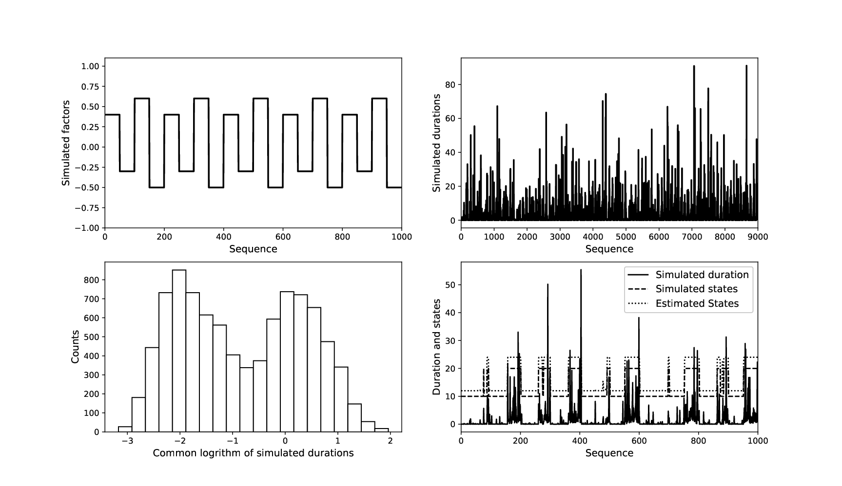
5 Real data analysis

5.1 Data cleaning and descriptive statistics

In the following, we implement the real data analysis for the inter-trade durations in the NASDAQ limit order market. The inter-trade durations usually contain the intra-day calendar effect, i.e., inter-trade durations tend to be shorter early and late in the day and longer around noon. Based on the standard dummy variable procedure (e.g.,Ghysels et al. 2004), we find that that the intra-day calendar effect is a common phenomena for all stocks in our sample (shown in Section E in the Appendices.). Therefore, prior to the analysis, we have adjusted inter-trade durations for the calendar effects.

For each stock in our sample, we aggregate the inter-trade durations in January 2013 and provide the descriptive statistics in Table 2. These statistics include count, min (the minimum), three quantiles, max (the maximum), mean, standard deviation, skewness, kurtosis, and over-dispersion (O.D.), which is the standard deviation divided by the mean. Table 2 suggests the following: 1) There is a large variation in their counts and maximum values; 2) The minimum values are approximately $10^{-6}$ seconds, and the mean values are approximately 1-10 seconds; 3) Their median value has a small variation, with most of them are around or below 0.1 seconds; and 4) They all exhibit a large dispersion as the values of their over-dispersion are significantly greater than one.

Table 2: Descriptive statistics of inter-trade durations for 25 NASDAQ stocks in January 2013.

Stock Count Min 25% Med. 75% Max Mean Std. Skew. Kurt. O.D. AAPL 539369 4.94E-06 7.51E-04 0.03 0.86 83.23 1.04 2.55 5.32 47.70 2.46 ALXN 88916 5.28E-06 1.09E-03 0.19 6.05 286.81 6.23 14.03 4.71 35.76 2.25 AMZN 171344 5.32E-06 5.03E-04 0.01 2.12 254.97 3.27 8.53 5.44 50.79 2.61 BIDU 102830 5.66E-06 9.97E-04 0.14 5.28 242.40 5.48 12.49 4.77 36.05 2.28 BMRN 47012 5.57E-06 6.56E-04 0.49 12.66 437.95 12.06 25.07 3.83 22.49 2.08 CELG 138826 5.00E-06 1.05E-03 0.11 4.18 213.83 4.06 8.66 4.13 28.22 2.13 CERN 44963 3.84E-06 1.05E-03 0.19 12.46 706.02 12.87 28.38 4.55 38.78 2.21 CMCSA 107143 5.93E-06 1.62E-03 0.16 4.64 601.18 5.29 12.88 6.42 101.10 2.43 COST 79533 6.51E-06 1.87E-03 0.44 7.73 444.95 6.81 13.88 4.84 56.97 2.04 DISCA 55283 5.72E-06 2.92E-03 0.82 11.16 425.82 10.06 20.41 4.09 28.31 2.03 EBAY 169875 6.39E-06 3.00E-03 0.21 3.52 363.80 3.47 7.61 5.44 76.51 2.20 FB 151244 4.34E-06 8.69E-04 0.08 3.20 294.02 3.92 9.88 5.80 59.27 2.52 GOOG 135745 5.50E-06 7.07E-04 0.06 3.75 235.97 4.05 9.16 4.34 29.78 2.26 INTC 124260 5.16E-06 1.00E-03 0.04 3.20 361.41 4.63 12.23 5.89 60.05 2.64 ISRG 38118 4.90E-06 4.43E-04 0.04 11.90 1504.86 15.02 37.79 6.45 102.77 2.52 KLAC 70264 5.17E-06 3.06E-03 0.54 9.21 600.68 8.31 17.46 5.68 83.42 2.10 MAR 39728 5.29E-06 3.03E-03 1.22 15.60 2166.25 14.02 31.83 15.83 795.34 2.27 MSFT 163839 5.91E-06 1.20E-03 0.05 2.50 833.87 3.72 10.69 10.40 348.43 2.87 NFLX 182071 5.05E-06 5.58E-04 0.03 2.41 242.51 3.34 8.47 5.17 43.02 2.54 QCOM 161471 6.86E-06 2.97E-03 0.26 3.75 443.04 3.54 7.71 6.08 115.19 2.18 REGN 52770 4.68E-06 4.76E-04 0.05 8.71 632.70 10.57 25.64 5.30 50.58 2.43 SBUX 101250 5.47E-06 3.52E-03 0.57 6.47 201.61 5.51 10.78 3.95 25.89 1.96 TXN 97907 5.28E-06 1.72E-03 0.27 5.73 461.87 5.87 13.20 5.04 49.99 2.25 VOD 57699 5.81E-06 3.86E-03 0.78 10.14 794.09 10.81 25.51 6.40 87.76 2.36 YHOO 91951 5.24E-06 1.63E-03 0.24 5.92 460.85 6.31 14.89 5.37 51.83 2.36

Note: 25%, Med., and 75% are the 25th percentile, 50th percentile (median), and 75th percentile, respectively. Std., Skew., and Kurt. are the standard deviation, skewness, and kurtosis, respectively.

5.2 Choice of LOB factors

To identify the factors that may impact the regime switchings of inter-trade durations, we focus the covariates in our model on the LOB factors for the following reasons. First, many studies advocate that the order flows are determined by the state of the order book (Hautsch and Huang 2012; Huang et al. 2015; Abergel and Jedidi 2015); therefore, factors reflecting the state of the LOB are thought to determine the flow of market orders and hence the inter-trade durations. Second, the information flow revealed by the change of LOB contribute a major part of information learning for the market participants (Harris and Panchapagesan 2005; Cao et al. 2009), especially for the HFTs who take the speed advantage to trade on the information. Third, a lot of research has found that the algorithm traders in the limit order market are indeed using LOB factors as signals to set their trading strategies. (Li et al. 2005; Obizhaeva and Wang 2013; Hendershott and Riordan 2013; Goldstein et al. 2018), so these factors must play an important role on the arrival time of trades, i.e., the inter-trade durations.

Let $p_{a}$ and $p_{b}$ be the prices (dollar prices divided by 10) for the best ask and the best bid, respectively, and $v_{a}^{1}$ and $v_{b}^{1}$ be the depth at the best ask and the best bid, respectively. We consider the following four LOB factors as the covariates in our MF-RSD model.

1.

Depth imbalance ( $DI$ ). $DI=\frac{|v_{a}^{1}-v_{b}^{1}|}{|v_{a}^{1}+v_{b}^{1}|}$ . It is the difference between the depth of the best ask and the depth of the best bid, divided by the sum of the two depths. It compares order supplies between the best ask and the best bid, and a large $DI$ reflects a great imbalance of the two sides in offering liquidity. Some studies (Cont et al. 2014; Lipton et al. 2013; Cartea et al. 2018) suggest that it is an effective predictor for the subsequent price movements and the rate of incoming orders.
2.

Price spread (PS). $PS=|p_{a}-p_{b}|$ , which is the price difference between the best ask and the best bid. It is commonly considered as a result of information asymmetry and reveals the stock’s overall liquidity (O’Hara 2003). From the perspective of market microstructure, it measures the transaction cost for the liquidity demander, and normally, a wider price spread implies weaker trading aggressiveness (Ranaldo 2004). Moreover, Carrion 2013 and Hendershott and Riordan 2013 found that high-frequency market makers provide liquidity when the spread is large while they take liquidity when the spread is small.
3.

Trade volume of the last trade, denoted by TV. It is the size of the last trade (volume measured in thousands), which is generally treated as a momentum variable that reflects the trading magnitude and willingness. Large trades normally convey more information than small trades (Hasbrouck 1991) and are also expected to be accompanied by some small upcoming trades (Van Kervel and Menkveld 2019).
4.

Price movement of the last trade, denoted by PM. It is a dummy variable that indicates whether the last trade had led to a change in mid-price, i.e., $\frac{p_{{}_{a}}+p_{b}}{2}$ . We think it might be a momentum variable for the price change and we want to see whether market participants treat it as an informative signal to identify the price movement in the following moments.

Table 3: Summary statistics for 4 LOB factors, which are depth imbalance (

DI

), price spread (

PS

), trade volume of the last trade (

TV

), and price movement of the last trade (

PM

Stock $DI$ $PS$ $TV$ $PM$ 25% Med 75% 25% Med 75% 25% Med 75% Mean AAPL 0.22 0.50 0.78 0.8 1.2 1.7 0.04 0.1 0.12 0.34 ALXN 0.16 0.37 0.71 0.3 0.5 0.7 0.05 0.1 0.1 0.38 AMZN 0.20 0.48 0.77 0.8 1.2 1.7 0.03 0.1 0.1 0.42 BIDU 0.20 0.39 0.71 0.3 0.4 0.7 0.09 0.1 0.15 0.43 BMRN 0.14 0.33 0.58 0.2 0.3 0.5 0.1 0.1 0.1 0.40 CELG 0.18 0.39 0.69 0.2 0.4 0.6 0.05 0.1 0.1 0.40 CERN 0.20 0.43 0.75 0.3 0.5 0.7 0.03 0.1 0.1 0.38 CMCSA 0.22 0.45 0.70 0.1 0.1 0.1 0.1 0.2 0.6 0.08 COST 0.20 0.40 0.66 0.2 0.2 0.3 0.05 0.1 0.12 0.36 DISCA 0.20 0.39 0.67 0.2 0.2 0.4 0.08 0.1 0.11 0.36 EBAY 0.23 0.48 0.72 0.1 0.1 0.2 0.1 0.17 0.34 0.18 FB 0.24 0.48 0.74 0.1 0.1 0.1 0.1 0.3 0.7 0.08 GOOG 0.19 0.49 0.79 1.7 2.6 3.7 0.02 0.09 0.1 0.40 INTC 0.22 0.46 0.74 0.1 0.1 0.1 0.1 0.3 1.2 0.03 ISRG 0.20 0.58 0.94 3.5 4.9 6.3 0.006 0.05 0.1 0.41 KLAC 0.20 0.42 0.66 0.1 0.2 0.2 0.1 0.1 0.2 0.30 MAR 0.20 0.41 0.64 0.1 0.1 0.2 0.1 0.1 0.2 0.29 MSFT 0.24 0.49 0.77 0.1 0.1 0.1 0.1 0.32 1.12 0.03 NFLX 0.14 0.38 0.68 0.9 1.4 2 0.07 0.1 0.11 0.45 QCOM 0.23 0.46 0.70 0.1 0.1 0.2 0.1 0.2 0.4 0.15 REGN 0.05 0.33 0.67 1.4 2 2.9 0.04 0.1 0.1 0.45 SBUX 0.21 0.44 0.68 0.1 0.1 0.2 0.1 0.1 0.26 0.22 TXN 0.24 0.50 0.74 0.1 0.1 0.1 0.1 0.2 0.5 0.11 VOD 0.31 0.60 0.84 0.1 0.1 0.1 0.1 0.28 0.7 0.09 YHOO 0.26 0.51 0.75 0.1 0.1 0.1 0.1 0.3 0.9 0.05

Note: 25%, Med., and 75% are the 25th percentile, 50th percentile (median), and 75th percentile, respectively.

In Table 3, we show some summary statistics of these LOB factors. The minimum and maximum values of $DI$ are 0 and 1, and the minimum values of $PS$ and $TV$ are always $0.1$ (1 cent) and $0.001$ (1 share), respectively; we do not report these values in the table. Since the factor $PM$ is a dummy variable, we only report its mean, or equivalently the ratio of the times when it equals to 1. From Table 3, we find that the percentiles of $DI$ are very similar across stocks. The factors $TV$ and $PM$ do have some differences from stock to stock, while the most divergent factor is $PS$ . For some stocks, such as CMCSA, FB, INTC, MSFT, TXN, VOD and YHOO, the factor $PS$ are most time fixed at 0.1 (the minimum tick size). But for some other stocks, such as GOOG, ISRG, and REGN, $PS$ varies much and its values can be very large.

5.3 In-sample regression and model prediction

We first implement the in-sample analysis for the inter-trade durations of MSFT on January 2, 2013, according to the following regression models for the transition probabilities:

	$\displaystyle\log\frac{P_{12}}{1-P_{12}}$	$\displaystyle=\beta_{12,0}+\beta_{12,1}DI+\beta_{12,2}PS+\beta_{12,3}TV+\beta_{12,4}PM,$		(12)
	$\displaystyle\log\frac{P_{21}}{1-P_{21}}$	$\displaystyle=\beta_{21,0}+\beta_{21,1}DI+\beta_{21,3}PS+\beta_{21,4}TV+\beta_{21,5}PM.$		(12)

The model is estimated using the EM procedure as described in Section 4 and the results are reported in Table 4. In addition to the full model - Model 6, we also estimate the submodels (Models 1-5). The distribution parameters estimated from the full model are very close to those from the submodels, and the estimated factor coefficients in the full model are having similar signs and significance levels as those in the submodels, suggesting that there is no strong multicollinearity in the LOB factors. In the rest of the empirical study, we shall only report the results using the full model (M6).

Table 4: Estimation results for MSFT on January 2, 2013, in 6 regression models.

Parameters	M1	M2	M3	M4	M5	M6
$\hat{\mu}_{1}$	0.131 (.0632)*	0.125 (.0602)*	0.132 (.0637)*	0.145 (.0690)*	0.131 (.0632)*	0.142 (.0670)**
$\hat{\lambda}_{1}$	0.000234 (5.45e-6)**	0.000234 (5.45e-6)**	0.000234 (5.45e-6)**	0.000234 (5.44e-6)**	0.000234 (5.45e-6**	0.000234 (5.44e-6)**
$\hat{\mu}_{2}$	10.066 (.418)**	10.070 (.419)**	10.062 (.418)**	10.025 (.423)**	10.065 (.418)**	10.024 (.422)**
$\hat{\lambda}_{2}$	2.411 (.109)**	2.407 (.109)**	2.403 (.109)**	2.324 (.106)**	2.409 (.109)**	2.318 (.105)**
$\hat{\beta}_{12,0}$	-1.061 (.0393)**	-0.424 (.0723)**	-0.781 (.120)**	-0.991 (.0459)**	-1.064 (.0407)**	0.881 (.177)**
$\hat{\beta}_{12,1}$	_	-1.249 (.128)**	_	_	_	-1.654 (.138)
$\hat{\beta}_{12,2}$	_	_	-2.237 (.913)*	_	_	-8.145 (1.118)**
$\hat{\beta}_{12,3}$	_	_	_	-0.0944 (.0368)*	_	-0.107 (.0350)**
$\hat{\beta}_{12,4}$	_	_	_	_	0.0479 (.156)	0.157 (.179)
$\hat{\beta}_{21,0}$	-0.442 (.0433)**	-0.925 (.0915)**	0.345 (.328)	-0.886 (.0569)**	-0.443 (.0432)**	-1.018 (.417)*
$\hat{\beta}_{21,1}$	_	0.947 (.158)**	_	_	_	1.139 (.168)**
$\hat{\beta}_{21,2}$	_	_	-7.685 (3.187)*	_	_	-4.539 (3.831)
$\hat{\beta}_{21,3}$	_	_	_	0.342 (.0320)**	_	0.341 (.0305)**
$\hat{\beta}_{21,4}$	_	_	_	_	0.345 (.692)	1.445 (.810)

Notes: M1 is a model without any LOB factor. M2-M5 are models having 1 LOB factor, with $DI$ , $PS$ , $TV$ and $PM$ , respectively. M6 is a model with all 4 LOB factors. The robust standard errors are shown in parentheses. $*p<0.05$ and $**p<0.01$ .

From Table 4, we can see that the estimated mean of the long-duration regime is much larger than that of the short-duration regimes, i.e., $\hat{\mu}_{2}>>\hat{\mu}_{1}$ . Based on the estimated values for the parameters of two IVGs, we also calculate the modes of the two distributions. They are around $8\times 10^{-5}$ seconds and $1$ second, which are consistent with the bimodal distribution of inter-trade durations discussed in Section 3. Moreover, we have noticed the following results for the LOB factors. First, the estimated coefficients for the $DI$ is significantly positive for ${P}_{12}$ ( $\hat{\beta}_{12,1}>0$ ) and significantly negative for ${P}_{21}$ ( $\hat{\beta}_{21,1}<0$ ). Second, the $PS$ is shown to be both negative for ${P}_{12}$ and ${P}_{21}$ while its coefficient is only significant in ${P}_{12}$ . Third, $\hat{\beta}_{12,3}$ is significantly less than 0 and $\hat{\beta}_{21,3}$ is significantly greater than 0, suggesting that the $TV$ is a significant factor for the regime switchings of inter-trade durations. Last, the factor $PM$ seems to be insignificant in this case because both $\hat{\beta}_{12,4}$ and $\hat{\beta}_{21,4}$ are not significantly different than 0. Nonetheless, the LOB factors fairly impact the dynamics of inter-trade duration via regime-switching probabilities, and we expect that our MF-RSD model can enhance the prediction of inter-trade durations by considering their effects. Moreover, we’d like to understand more about the economics implication of the effects of LOB factors on the regime switchings of inter-trade durations, which will be discussed in detail in Section 5.5.

Given the estimated values of model parameters, we examine the model prediction power by first considering a 1-step-ahead out-of-sample prediction for the underlying states. The 1-step-ahead prediction of $s_{i}$ is given by

	$\displaystyle\mathrm{E}_{i}(s_{i+1})$	$\displaystyle=1\cdot\left[\mathbb{P}(s_{i}=1\|\mathcal{F})\hat{P}_{11,i+1}+\mathbb{P}(s_{i}=2\|\mathcal{F})\hat{P}_{21,i+1}\right]$		(13)
		$\displaystyle+2\cdot\left[\mathbb{P}(s_{i}=1\|\mathcal{F})\hat{P}_{12,i+1}+\mathbb{P}(s_{i}=2\|\mathcal{F})\hat{P}_{22,i+1}\right],$		(13)

and the transition probabilities at $i$ are given by

	$\displaystyle\log\frac{\hat{P}_{12,i+1}}{1-P_{12,i+1}}$	$\displaystyle=\hat{\beta}_{12,0}+\hat{\beta}_{12,1}DI_{i}+\hat{\beta}_{12,2}PS_{i}+\hat{\beta}_{12,3}TV_{i}+\hat{\beta}_{12,4}PM_{i}$		(14)
	$\displaystyle\log\frac{\hat{P}_{21,i+1}}{1-P_{21,i+1}}$	$\displaystyle=\hat{\beta}_{21,0}+\hat{\beta}_{21,1}DI_{i}+\hat{\beta}_{21,2}PS_{i}+\hat{\beta}_{21,3}TV_{i}+\hat{\beta}_{21,4}PM_{i}.$		(14)

which can be calculated given the information up to $i-$ th trade.

We use the MSFT inter-trade duration series on January 2, 2013, to demonstrate the above prediction. The model parameter is estimated using the first 5000 samples, and 1-step-ahead forecasting is made for the next 200 durations. Figure 6 shows the comparison between the estimated states and the 1-step-ahead forecasts. The estimated states are the underlying states inferred from the real data, and the forecasted states are 1-step-ahead out-of-sample prediction.⁷⁷ 7 The states jump between two values, i.e., state 1 (the short-duration regime) and state 2 (the long-duration regime) From the result, we can see that the forecasted states almost capture the variation tendency of the underlying estimated states.

Furthermore, the 1-step-ahead prediction for the inter-trade duration is expressed as

	$\displaystyle\mathrm{E}_{n}(y_{n+1})$	$\displaystyle=\hat{\mu}_{1}\cdot\left[\mathbb{P}(s_{n}=1\|\mathcal{F})\hat{P}_{11,n+1}+\mathbb{P}(s_{n}=2\|\mathcal{F})\hat{P}_{21,n+1}\right]$		(15)
		$\displaystyle+\hat{\mu_{2}}\cdot\left[\mathbb{P}(s_{n}=1\|\mathcal{F})\hat{P}_{12,n+1}+\mathbb{P}(s_{n}=2\|\mathcal{F})\hat{P}_{22,n+1}\right].$		(15)

To see the predictive performance of our model, we compare our results in predicting the next inter-trade duration with those of two classical duration models, i.e., the ACD model by Engle and Russell 1998 and the MSMD model by Chen et al. 2013. The ACD model we considered has the following form:

y_{i}=\varphi_{i}\varepsilon_{i},\qquad\varphi_{i}=\omega+\alpha y_{i-1}+\beta\varphi_{i-1},

where $\varepsilon_{i}$ follows an inverse Gaussian distribution. The MSMD model we considered has five levels, and the following form:

	$\displaystyle y_{i}$	$\displaystyle=\frac{\varepsilon_{i}}{\lambda_{i}}=\varphi_{i}\varepsilon_{i},\quad\varphi_{i}=\varphi\prod_{k=1}^{5}M_{k,i},$
	$\displaystyle M_{k,i}$	$\displaystyle=\begin{cases}M&\textrm{w.p. }1-(1-\gamma_{5})^{b^{k-5}}\\ M_{k,i-1}&\textrm{w.p. }(1-\gamma_{5})^{b^{k-5}}\end{cases}\quad k=1\ldots 5,\quad M=\begin{cases}m_{0}&\textrm{w.p. }1/2\\ 1-m_{0}&\textrm{w.p. }1/2\end{cases}$

in which $\varepsilon_{i}$ also follows an inverse Gaussian distribution.

Table 5 shows the comparison among our model, the ACD(1,1) model and the MSMD(5) model. We use the BIC as an indicator to compare their in-sample fitness. From the results, we find that the in-sample fitness of our MF-RSD model is slightly worse than that of the ACD(1,1) model but better than that of the MSMD(5) model. This is probably because the ACD model has the most parsimonious structure and the least number of parameters. For the out-of-sample prediction power, we use the RMSE between the real duration and the predicted duration as a measurement. Nonetheless, from the results in Table 5, our MF-RSD model performs significantly better than the other two models.

Table 5: The evaluation of in-sample fitness and out-of-sample forecast for 25 NASDAQ stocks on January 2, 2013, with a benchmark comparison to the ACD and MSMD models.

Log-likelihood BIC RMSE Stock $n$ MF-RSD ACD MSMD MF-RSD ACD MSMD MF-RSD ACD MSMD AAPL 28888 35421.60 35936.97 30748.48 -70699.41 -71812.31 -61445.60 1.91 2.00 2.91 ALXN 5240 -704.66 -318.01 -1365.19 1529.22 687.40 2773.20 8.21 9.38 9.54 AMZN 7674 5901.71 5876.18 5024.88 -11678.18 -11698.69 -10005.03 6.95 7.14 8.37 BIDU 3819 -4467.04 -4130.39 -4685.14 9049.55 8310.27 9411.52 12.09 13.39 18.05 BMRN 2892 -2729.22 -2435.24 -3127.84 5570.02 4918.29 6295.53 15.75 18.96 21.25 CELG 4717 -3832.10 -3420.28 -3498.79 7782.63 6891.31 7039.87 8.54 9.72 9.81 CERN 2460 -2424.12 -2202.68 -1316.67 4957.55 4452.21 2672.38 15.50 19.07 29.18 CMCSA 5235 -2031.46 -1933.45 -1778.63 4182.80 3918.28 3600.08 11.11 12.56 12.61 COST 4330 -4394.69 -4125.27 -4907.93 8906.61 8300.78 9857.73 8.96 10.22 10.67 DISCA 3055 -1062.11 -891.86 -919.68 2236.57 1831.87 1879.49 16.66 16.92 17.96 EBAY 9697 1450.65 2098.67 -484.82 -2772.79 -4142.26 1015.53 5.78 5.59 6.04 FB 10278 8222.19 8579.60 5865.68 -16315.06 -17103.77 -11685.17 5.13 5.46 7.06 GOOG 6387 4725.22 4715.50 -6186.30 -9327.78 -9378.43 12416.41 8.13 8.44 8.59 INTC 5300 2149.62 2144.01 10.61 -4179.19 -4236.57 21.66 11.27 12.20 12.11 ISRG 1918 -1128.08 -1028.33 -715.34 2361.99 2094.46 1468.48 25.72 27.33 30.48 KLAC 3059 -3076.43 -2749.82 -2536.58 6265.23 5547.80 5113.29 14.32 16.17 26.80 MAR 2404 -3733.69 -3430.79 -3801.85 7576.38 6908.28 7642.62 21.91 22.42 26.41 MSFT 6242 3472.11 3354.70 2887.86 -6821.88 -6656.96 -5732.03 8.19 9.57 9.91 NFLX 3594 -2158.32 -1800.04 -4272.06 4431.27 3649.20 8585.06 10.98 12.89 13.33 QCOM 8726 -2759.03 -2061.64 -6911.35 5645.10 4177.72 13868.07 5.35 5.85 6.04 REGN 3841 860.04 999.03 808.91 -1604.53 -1948.53 -1576.55 10.89 12.56 12.88 SBUX 5740 -3886.73 -3290.91 -4722.18 7894.64 6633.76 9487.64 7.10 7.76 8.64 TXN 5633 -1794.99 -1412.53 -3939.81 3710.88 2876.88 7922.80 9.38 11.01 11.07 VOD 1810 -2257.49 -2259.32 -2312.70 4619.99 4563.65 4662.91 42.13 44.50 45.61 YHOO 3797 1223.24 1195.00 -611.21 -2331.08 -4109.70 1263.63 16.69 15.74 16.48

Note: BIC= $k*\ln n-2*\ln\hat{L}$ , where $\hat{L}$ is the likelihood. The lower value BIC is, the better the in-sample fitness. The RMSE is the square root of MSE, and the lower the value is, the better the out-of-sample performance.

5.4 Analysis of regimes

In the next, we want to see the characteristics of the underlying regimes that are estimated from our MF-RSD model. In Figure 7, we plot the first MSFT 300 inter-trade durations on January 2, 2013, along with their estimated levels of the underlying regimes. It shows that the estimated regimes capture the clustering of the long (or short) inter-trade durations, and there are significant switchings between the long-duration regime and the short-duration regime. Given the estimated underlying regimes, we will diagnose the two regimes and check whether they are related to different channels of profitability for the HFTs, because we think that in the long-duration regime, HFTs mainly provide liquidity and gain profit from the price spread as market makers, while in the short-duration regime, HFTs aggressively take liquidity and earn profit as speculators because of the short-term price movement.

To make things comparable, we divide the trading day into 360 one-minute intervals and calculate the ratio of the number of short inter-trade durations to the total number of trades in each interval, which is defined as the HF ratio. We categorize the short and long inter-trade durations based on which regime they belong to. The LF ratio is then defined as the ratio of long inter-trade durations and hence equals to 1-HF ratio. Thus, a high HF (LF) ratio means that the short-duration (long-duration) regime is dominated in the interval. Following Carrion 2013, we use the permanent price change and the realized price spread as the metrics of profit. The permanent price change is defined as the absolute percentage change of midpoint price in the one-minute interval, which measures the profit of taking liquidity, and the realized price spread is the average effective price spread minus the permanent price change, which measures the profit of supplying liquidity. We also include the order submission rate and the cancellation rate to see the market activity level. As the time length of the interval is fixed, we simply use the numbers of submissions and cancellations in one minute to represent the rates.

We still use MSFT on January 2, 2013 as an example. For each one-minute interval, we calculate the HF ratio, the LF ratio, the order submissions, the order cancellations, the permanent price change, and the realized price spread. In Table 6, we present their correlation matrix, from which we can observe that the HF ratio is positively correlated with the order submissions, cancellations, and the permanent price change, but negatively correlated with the realized price spread. The LF ratio is having the opposite relationships with those 4 metrics. Thus, the profit of taking liquidity is large when the market in the short-duration regime in which the HFTs are using aggressive trading strategies. While in the period with a high LF ratio, i.e., when HFTs mainly supply liquidity, the profit of supplying liquidity is larger as the realized price spread is positively correlated with the LF ratio.

Table 6: Pearson correlation matrix for the HF ratio, the LF ratio, the order submissions, cancellations, the permanent price change and the realized price spread.

HF ratio LF ratio Cancel Submit Price Realized change spread HF ratio 1 LF ratio -1 1 Cancel 0.472** -0.472** 1 Submit 0.474** -0.474** 0.998** 1 Price change 0.366** -0.366** 0.457** 0.463** 1 Realized spread -0.298** 0.298** -0.330** -0.337** -0.982** 1

*p<0.05, **p<0.01

Furthermore, we implement the below regression to see which regime or which regime-switching action is followed by a significant short-term price movement.

\Delta P_{i,t(+10s)}=constant+\mathbf{1}_{s_{i}=1}+\hat{P}_{12,i+1}+\hat{P}_{21,i+1}+\varepsilon_{it}

(16)

In the regression, $\Delta P_{i,t(+10s)}$ is the absolute value of the percentage change of midpoint price in the next 10 seconds after $i-$ th trade.⁸⁸ 8 As we mainly care about the HFTs’ behaviors, we think 10 seconds is long enough at the high-frequency level. $\mathbf{1}_{s_{i}=1}$ is the indicator which equals to 1 if the $i-$ th trade belongs to the short-duration regime. $\hat{P}_{12,i+1}$ is the estimated transition probability for the next inter-trade duration switching from the short-duration regime to the long-duration regime, and $\hat{P}_{21,i+1}$ is the estimated regime transition probability for the next inter-trade duration on the contrary; both of them are calculated by equation (14) according to our MF-RSD model.

Table 7: The regressions of the short-term price change on the short-duration regime and regime-switching probabilities

$\Delta P$ $\Delta P$ $\Delta P$ $\Delta P$ $\mathbf{1}_{s_{i}=1}$ .0032 .0037 (.001)* (.001)** $\hat{P}_{12,i+1}$ -.0131 .0027 (.005)* (.006) $\hat{P}_{21,i+1}$ .0124 .0146 (.003)** (.004)** $constant$ .0377 .0431 .0350 .0312 (.001)** (.001)** (.001)** (.003)**

Note: $\Delta P$ is the percentage change of mid-price in the next 10 seconds. The robust standard errors are shown in parentheses. $*p<0.05$ and $**p<0.01$ .

The regression results are presented in Table 7. From it, we can see that the coefficient for $\mathbf{1}_{s_{i}=1}$ is positive. Hence the short-duration regime will be followed by a larger price change compared with the long-duration regime. Nonetheless, from the last column of Table 7, we note that the effect for the transition probability from the long-duration regime to the short-duration regime is even stronger, as the coefficient of $\hat{P}_{21,i+1}$ is significantly greater than the coefficient of $\mathbf{1}_{s_{i}=1}$ . This means that a large price change follows the short-duration regime, while a stronger price movement will occur subsequently if the market is switching from the long-duration regime to the short-duration regime. We think this switching could be predicted by the HFTs, so they would take this opportunity to trade on the signal and to earn a profit as price speculators. However, the effect for $\hat{P}_{12,i+1}$ is not significant, so the price change is relatively small if the HFTs turn from the aggressive trading strategy to the passive one.

5.5 Analysis of LOB factors

At last, we have studied the informativeness of LOB factors to the trading activities by applying the MF-RSD model to the 25 NASDAQ stocks in our sample for 21 trading days (January 2013). For each stock and each factor, we count the number of days in which the factor coefficient in the regression (12) is significant. The results are presented in Table 8 and the main findings are as follows.

Table 8: Summary of the results for the significance of 4 LOB factors in the MF-RSD model.

Stock $DI$ $PS$ $TV$ $PM$ $\mathrm{P_{12}}$ $\mathrm{P_{21}}$ $\mathrm{P_{12}}$ $\mathrm{P_{21}}$ $\mathrm{P_{12}}$ $\mathrm{P_{21}}$ $\mathrm{P_{12}}$ $\mathrm{P_{21}}$ sig(+) sig(-) sig(+) sig(-) sig(+) sig(-) sig(+) sig(-) sig(+) sig(-) sig(+) sig(-) sig(+) sig(-) sig(+) sig(-) AAPL 0 13 1 2 21 0 0 21 0 11 21 0 21 0 9 0 ALXN 3 1 1 4 7 0 0 19 0 10 9 1 20 0 0 21 AMZN 1 2 4 0 17 0 0 21 0 9 15 0 21 0 0 21 BIDU 1 0 1 0 13 0 0 19 0 4 16 0 21 0 0 21 BMRN 0 0 3 0 9 1 0 21 0 6 11 0 15 0 0 12 CELG 0 3 6 0 4 2 0 14 0 13 20 0 21 0 0 21 CERN 1 0 1 1 7 0 0 18 0 4 9 0 21 0 0 20 CMCSA 0 17 19 0 1 12 0 7 0 16 21 0 11 0 6 0 COST 3 2 1 0 4 4 0 15 0 12 20 0 21 0 0 21 DISCA 0 2 1 0 2 1 0 17 0 8 17 0 19 0 0 19 EBAY 1 3 0 6 10 0 0 21 0 18 20 0 20 0 0 3 FB 0 12 2 2 14 3 0 21 0 16 21 0 20 0 9 0 GOOG 1 4 2 1 21 0 0 21 0 12 20 0 21 0 0 18 INTC 0 20 18 0 0 15 1 3 0 14 20 0 2 5 5 0 ISRG 1 1 0 2 10 3 0 20 5 0 11 0 18 0 1 12 KLAC 0 6 2 1 5 3 0 17 0 11 15 0 12 0 0 11 MAR 0 10 4 0 1 4 0 11 0 9 16 0 10 0 2 4 MSFT 0 20 20 0 1 17 1 2 0 13 20 0 1 6 5 0 NFLX 0 6 7 0 13 1 0 21 0 12 19 0 21 0 0 18 QCOM 0 11 4 0 5 1 0 21 0 20 21 0 15 0 4 6 REGN 0 12 9 0 17 1 0 21 1 0 9 0 21 0 0 19 SBUX 0 14 4 0 2 5 0 15 0 17 21 0 11 0 0 3 TXN 0 13 8 0 1 3 0 8 0 11 21 0 9 0 2 1 VOD 0 15 17 0 3 2 0 0 1 1 19 0 9 0 1 0 YHOO 0 21 19 0 1 9 3 2 0 12 21 0 2 5 6 0 Sum (%) 2.3% 39.6% 29.3% 3.6% 36.0% 16.6% 1.0% 71.6% 1.3% 49.3% 82.5% 0.2% 73.0% 3.0% 9.5% 47.8%

Note: $P_{12}$ represents the regime switching from the short-duration regime to the long-duration regime, and $P_{21}$ represents the regime switching from the long-duration regime to the short-duration regime. Significance is measured at the 5% level. Sig(+)/Sig(-) means that the estimated coefficient for the factor is significantly positive/negative. Each cell shows the counts of significance. We have 21 trading days for each stock, so the upper limit for each cell is 21. The last row records the percentage (%) of the times that this factor appears as significant in all 525 instances (25 stocks times 21 days).

1.

The effect of $DI$ : in approximately 40% of total instances, it is significantly negative for $P_{12}$ , and in approximately 30% of total instances, it is significantly positive for $P_{21}$ . Hence, the effect of depth imbalance between the best ask and the best bid on the regime-switching probabilities is not very common. Nevertheless, for the stocks which have very tight price spread, $DI$ has a common effect. For instance, we have summarized the results for the stocks whose price spread mostly keep at 0.1, including CMCSA, FB, INTC, MSFT, TXN, VOD, and YHOO, and find that $DI$ is significantly negative for $P_{12}$ in 80% of total occurrences and significant positive for $P_{21}$ in 70% of total occurrences. Thus, we think that the impact of $DI$ on the dynamics of inter-trade durations is price spread dependent. When price spread is tight, the effect of $DI$ is significant, i.e., the greater the depth imbalance is, the inter-trade durations are more likely to stay in (or switch to) the short-duration regime.
2.

The effect of $PS$ : it is not obvious for $P_{12}$ , but it is significantly negative for $P_{21}$ in more than 70% of total instances. Thus, the effect of the price spread between the best ask and the best bid on the inter-trade durations switching from the short-duration regime to the long-duration regime is ambiguous, while it is commonly significantly negative for the switching from the long-duration regime to the short-duration regime. This means that the larger the price spread is, it is more likely that the inter-trade durations that were previously in the long-duration regime keep staying in the long-duration regime.
3.

The effect of $TV$ : it is significantly negative for $P_{12}$ in nearly 50% of total instances and is significantly positive for $P_{21}$ in 82% of total instances. Thus, the larger quantity the last trade has, the more likely that the short inter-trade durations stay in the preceding short-duration regime. Also, a larger quantity of trade is more likely to lead the inter-trade durations that were previously in the long-duration regime to switch to the short-duration regime.
4.

The effect of $PM$ : it is significantly positive for $P_{12}$ in 73% of total instances and is significantly negative for $P_{21}$ in nearly 50% of total instances. Hence, whether the mid-price has changed in the previous trade has an important effect on the regime-switching probabilities. It is commonly significantly positive for the inter-trade durations switching from the short-duration regime to the long-duration regime, which means that if mid-price has moved, inter-trade durations are very likely to switch to the long-duration regime. Also in many cases, it is significantly negative for the inter-trade durations switching from the long-duration regime to the short-duration regime, which means that if the mid-price moves, inter-trade durations are inclined to stay in the preceding long-duration regime.

Some of our findings are in harmony with those of the existing research on market microstructure. First, many papers (Li et al. 2005; Goldstein et al. 2018; Van Kervel and Menkveld 2019) suggest that order imbalance is a good predictor for price movement, and algorithm traders would use it as a trading indicator. A larger imbalance is a signal for future price movement and hence encourages traders (in particular HFTs) to actively trade to gain profit (or prevent loss). This is why, in some cases, the effect of depth imbalance is significantly negative for inter-trade durations switching from the short-duration regime to the long-duration regime and significantly positive for the switching from the long-duration regime to the short-duration regime. Second, according to (Ranaldo 2004; Carrion 2013; Hendershott and Riordan 2013), price spread is an indicator of liquidity and measures the profit (cost) of providing (taking) liquidity. A large price spread indicates illiquidity of the asset, and the larger the price spread is, the more transaction cost liquidity takers face and meanwhile the more profit liquidity providers have. Thus, when the price spread becomes larger, people are more reluctant to initialize market orders and the inter-trade durations are more likely to be long. Third, trade volume is indeed a momentum variable that reflects trading willingness (O’hara 1995; Hasbrouck 1991). A large trade volume would not only keep the market in an active trading period (the short-duration regime) but also lead the market to switch from a passive trading period to an active one. Finally, the effect of price movement seems to violate the negative correlation between price movement and duration length (Manganelli 2005; Furfine 2007). However, in our high-frequency data, perhaps the change in mid-price in the last trade is not a momentum variable for future price movement. Moreover, we find that the change in mid-price just occurs because the existing limit orders at best bid or best ask are eliminated by the incoming trade, and consequently the price spread between the best ask and the best bid increases. Thus, we suspect that its effect on the regime switchings of inter-trade durations is probably resulted from another channel, i.e., an increase in the price spread.

In addition, we obtain some new findings. First, the depth imbalance plays an important role mostly when the price spread is small. A possible explanation is that when the price spread is large, the depth imbalance is less informative as it is relatively costless for traders to submit orders at the best ask/bid. Moreover, within the revealed price spread, perhaps there are some hidden limit orders that make the true depth imbalance between the best ask and the best bid unknowable. Only when the price spread is tight, the depth imbalance reveals more information and becomes a valid indicator for the subsequent price movement. Next, a large price spread is more likely to keep inter-trade durations in the long-duration regime rather than to reverse inter-trade durations from the short-duration regime to the long-duration regime, as we have observed that the effect of price spread is commonly negative for $P_{21}$ but is not obvious for $P_{12}$ . This finding suggests that traders are more sensitive to the size of $PS$ when the market is in the long-duration regime, in which HFTs mainly provide liquidity and slow traders consume liquidity. The slow traders seem to be more concerned with a high transaction cost induced by a large $PS$ when the market is relatively stable. However, when the market enters the short-duration regime in which HFTs aggressively take liquidity and earn a profit because of the price movement, a large price spread would not impede the HFTs’ trading aggressiveness and play a significant role in the arrival time of trades. Finally, as the effect of $PM$ is commonly positive for $P_{12}$ and $PM=1$ is accompanied by an increase of price spread, whether the price spread has just increased could be a driving force that leads inter-trade durations to switch to the long-duration regime. This finding may affirm the viewpoint in Obizhaeva and Wang 2013 that the optimal strategy for algorithm traders depends more on the resilience properties of supply/demand such as the change in bid-ask spread, rather than its static property.

To further verify the mechanism of LOB factors on the dynamics of inter-trade durations and our explanation, we implement the below ‘naive’ panel data regression to see the relationship between the LOB factors and the price change in the next 10 seconds. The regression model is like following:

\Delta P_{i,t(+10s)}=constant+DI_{i,t}+PS_{i,t}+TV_{it}+PM_{it}+\mu_{i}+\varepsilon_{it}

(17)

where $i$ and $t$ indicate the $i-$ th stock and the $t-$ th trade respectively, and $\Delta P$ is the short-term price change, the same as in the equation 16. Here we just use the data of 25 stocks on the same day, i.e., January 2, 2013. The panel data is unbalanced because different stocks have different numbers of trades.

Table 9: The regressions of the short-term price change on the LOB factors

Full Sample Subsample Subsample (tight spread) (slack spread) $\Delta P$ $\Delta P$ $\Delta P$ $\Delta P$ DI .00192 .00208 .00672** -.000325 (.00119) (.00113) (.00217) (.000597) PS .00436** (.00100) TV .00188** .00189** .00186** .0140* (.000199) (.000201) (.000192) (.005034) PM -.00192 -.000890 .00215* -.00139* (.000626) (.000481) (.000782) (.000603) constant .0235** .0268** .02242** .0285** (.00102) (.000542) (.00112) (.000290) fixed effect Y Y Y Y number of stocks 25 25 12 13 observations 146,736 146,736 67,921 78,815

Note: Panel data regression with fixed effect. $\Delta P$ is the percentage change of mid-price in the next 10 seconds. The robust standard errors are shown in parentheses. $*p<0.05$ and $**p<0.01$ .

The regression results are presented in Table 9. As we can see, for the full sample, the LOB factor $DI$ and $PM$ don’t show a significant effect on the price change. This finding advocates that the depth imbalance is overall not informative and the price movement of last trade is not a momentum variable for the future price movement. Nevertheless, a large $TV$ predicts a large price change because the $TV$ is significantly positive for the $\Delta P$ , which is in line with our finding that a large trade volume will induce short inter-trade durations as HTFs treat it as a signal for future price movement. The coefficient of $PS$ is significant and positive for $\Delta P$ , however, we think the $PS$ could be endogenously correlated with the price change as the effective price spread ( $PS$ ) consists of the permanent price change ( $\Delta P$ ) and the realized price spread, which compensate liquidity providers costs on two aspects, i.e., the adverse select cost and the ‘real friction’ (Carrion 2013). Thus, we exclude $PS$ in the second regression and the result shows that the other three LOB factors have similar effects. We further divided the 25 stocks into two subgroups to verify the effect of $DI$ . One subgroup has stocks with relatively tight price spreads,⁹⁹ 9 There are 12 stocks in total. 75% percentile of the $PS$ for each stock is less than or equal to 0.2. the other subgroup has the remaining stocks, whose price spreads are relatively slack. From the last two columns in Table 9, we can observe that the $DI$ in the first subgroup is significantly positive, while it is insignificant in the second subgroup. The finding strongly supports the conclusion that the depth imbalance is informative and a valid indicator for HFTs only when the price spread is small, and a large depth imbalance in such case is very likely to indicate the following price movement.

Moreover, we have provided robustness tests for the findings on the effects of the LOB factors. The tests include the analysis of NASDAQ stocks in a different month, the analysis of directional trades, the analysis of $DI$ conditional on the tightness of $PS$ , the analysis with a substitution of $DI$ by the aggregated depth imbalance, and the analysis with a substitution of $PM$ by a dummy variable for the increase in price spread. These robustness test are presented in Section F the Appendices, and the results are very consistent with our findings.

6 Conclusion

In this paper, we have proposed a multifactor regime-switching duration (MF-RSD) model for the inter-trade durations in the high-frequency limit order market. The motivation is that we have found a common bimodal distribution of inter-trade durations for the stocks listed in the NASDAQ market. The simulation study of MF-RSD model not only validates our estimation method but also shows that the model can replicate the most empirical facts of inter-trade durations, including the newly found bimodal distribution. Furthermore, based on the empirical analysis, we find that the underlying regimes are related to the endogenous liquidity provision and consumption by the HFTs in the market. Using the factor analysis, the MF-RSD model is also capable to identify the types of market information that algorithm traders learn from and react to in high frequency, which causes the inter-trade durations switching between the short-duration and the long-duration regime.

The contribution of the MF-RSD model in analyzing the high-frequency inter-trade duration data in the LOB can be summarized in the following three aspects. First, the out-of-sample test shows that the performance of the MF-RSD model in predicting inter-trade durations is significantly improved compared with the two benchmark duration models. This is because, through the identified impacts of the LOB factors and the parsimonious structure of the two regimes, our model is able to predict whether the arrival time of the next trade is relatively long or short. Second, given the estimated regimes and the estimated regime-switching probabilities by the MF-RSD model, we find empirical evidence that the switchings between the short-duration regime and the long-duration regime result from the HFTs’ behavior of changing strategies between providing liquidity and taking liquidity, driven by the different channels of profitability. Specifically, the short-duration regime is followed by a relatively large price movement, which corresponds to a high profit of taking liquidity, while the long-duration regime is positively correlated with the realized price spread, which measures the profit of providing liquidity. Third, the MF-RSD model is also useful in testing economic hypotheses in the market microstructure theory, and our results are consistent with some findings in the prevalent literature. They are as follows: 1) order book imbalance is applicable to predict the price movement in the short term, and in some cases, a larger depth imbalance would lead to a shorter inter-trade duration; 2) a larger price spread tends to maintain inter-trade duration in the long-duration regime because it reflects higher transaction costs for liquidity demanders; and 3) a larger trade volume is a good momentum variable that reveals a strong trading willingness, which normally induces a shorter duration for the next trade. Moreover, we have some new findings added to the literature. They are: 1) the impact of depth imbalance on the regime-switching of inter-trade duration is spread-dependent and is significant when the stock’s price spread is tight; 2) a large price spread is not a reverse signal for inter-trade durations switching from the short-duration regime to the long-duration regime if they were staying in the short-duration regime; and 3) whether the price spread has just increased in the last trade is nonetheless a reverse signal for the regime switching of inter-trade durations, through our analysis of the impact of the mid-price movement.

Our work has made progress in analyzing the high-frequency duration data. Nevertheless, it leaves a great deal to future research. For example, our LOB data is rich in terms of having records of order submissions and cancellations, we can further investigate the impact of those activities on the arrival time of trades. To achieve that, a new econometric model is probably needed. Moreover, some event studies could be implemented to directly identify the HFTs’ behaviors of switching trading strategies if we can obtain the data that contain exogenous shocks to the market, which helps to verify our findings on the regime-switching of inter-trade durations. We can also test whether inter-trade durations in other high-frequency financial markets have similar properties, in particular, whether the bimodal distribution is a general phenomenon, and a theoretical market microstructure model is certainly needed if so.

References

Abergel and Jedidi (2015) Abergel, F. and A. Jedidi
2015. Long-time behavior of a hawkes process–based limit order book. SIAM Journal on Financial Mathematics, 6(1):1026–1043.
Aliyev et al. (2018) Aliyev, N., X. He, and T. J. Putniņš
2018. Learning about toxicity: Why order imbalance can destabilize markets. Available at SSRN.
Bauwens and Giot (2000) Bauwens, L. and P. Giot
2000. The logarithmic acd model: an application to the bid-ask quote process of three nyse stocks. Annales d’Economie et de Statistique, Pp. 117–149.
Bauwens and Giot (2003) Bauwens, L. and P. Giot
2003. Asymmetric acd models: introducing price information in acd models. Empirical Economics, 28(4):709–731.
Bauwens and Veredas (2004) Bauwens, L. and D. Veredas
2004. The stochastic conditional duration model: a latent variable model for the analysis of financial durations. Journal of econometrics, 119(2):381–412.
Brogaard et al. (2014) Brogaard, J., T. Hendershott, and R. Riordan
2014. High-frequency trading and price discovery. The Review of Financial Studies, 27(8):2267–2306.
Cao et al. (2009) Cao, C., O. Hansch, and X. Wang
2009. The information content of an open limit-order book. Journal of Futures Markets: Futures, Options, and Other Derivative Products, 29(1):16–41.
Carrion (2013) Carrion, A.
2013. Very fast money: High-frequency trading on the nasdaq. Journal of Financial Markets, 16(4):680–711.
Cartea et al. (2018) Cartea, Á., R. Donnelly, and S. Jaimungal
2018. Enhancing trading strategies with order book signals. Applied Mathematical Finance, Pp. 1–35.
Chang et al. (2017) Chang, Y., Y. Choi, and J. Y. Park
2017. A new approach to model regime switching. Journal of Econometrics, 196(1):127–143.
Chen et al. (2013) Chen, F., F. X. Diebold, and F. Schorfheide
2013. A markov-switching multifractal inter-trade duration model, with application to us equities. Journal of Econometrics, 177(2):320–342.
Cont et al. (2014) Cont, R., A. Kukanov, and S. Stoikov
2014. The price impact of order book events. Journal of financial econometrics, 12(1):47–88.
Deo et al. (2010) Deo, R., M. Hsieh, and C. M. Hurvich
2010. Long memory in intertrade durations, counts and realized volatility of nyse stocks. Journal of Statistical Planning and Inference, 140(12):3715 – 3733.
Diebold and Inoue (2001) Diebold, F. X. and A. Inoue
2001. Long memory and regime switching. Journal of econometrics, 105(1):131–159.
Diebold et al. (1994) Diebold, F. X., J.-H. Lee, and G. C. Weinbach
1994. Regime switching with time-varying transition probabilities. Business Cycles: Durations, Dynamics, and Forecasting, Pp. 144–165.
Došlá (2009) Došlá, Š.
2009. Conditions for bimodality and multimodality of a mixture of two unimodal densities. Kybernetika, 45(2):279–292.
Engle (2000) Engle, R. F.
2000. The econometrics of ultra-high-frequency data. Econometrica, 68(1):1–22.
Engle and Russell (1998) Engle, R. F. and J. R. Russell
1998. Autoregressive conditional duration: a new model for irregularly spaced transaction data. Econometrica, Pp. 1127–1162.
Foster et al. (2019) Foster, F. D., X. He, J. Kang, and S. Lin
2019. The microstructure of endogenous liquidity provision. Available at SSRN.
Furfine (2007) Furfine, C.
2007. When is inter-transaction time informative? Journal of Empirical Finance, 14(3):310–332.
Ghysels et al. (2004) Ghysels, E., C. Gourieroux, and J. Jasiak
2004. Stochastic volatility duration models. Journal of Econometrics, 119(2):413–433.
Glosten and Milgrom (1985) Glosten, L. R. and P. R. Milgrom
1985. Bid, ask and transaction prices in a specialist market with heterogeneously informed traders. Journal of financial economics, 14(1):71–100.
Goldstein et al. (2018) Goldstein, M. A., A. Kwan, and R. Philip
2018. High-frequency trading strategies.
Hagströmer and Nordén (2013) Hagströmer, B. and L. Nordén
2013. The diversity of high-frequency traders. Journal of Financial Markets, 16(4):741–770.
Harris and Panchapagesan (2005) Harris, L. E. and V. Panchapagesan
2005. The information content of the limit order book: evidence from nyse specialist trading decisions. Journal of Financial Markets, 8(1):25–67.
Hasbrouck (1991) Hasbrouck, J.
1991. Measuring the information content of stock trades. The Journal of Finance, 46(1):179–207.
Hasbrouck and Saar (2013) Hasbrouck, J. and G. Saar
2013. Low-latency trading. Journal of Financial Markets, 16(4):646–679.
Hautsch (2011) Hautsch, N.
2011. Econometrics of financial high-frequency data. Springer Science & Business Media.
Hautsch and Huang (2012) Hautsch, N. and R. Huang
2012. The market impact of a limit order. Journal of Economic Dynamics and Control, 36(4):501–522.
Hendershott and Riordan (2013) Hendershott, T. and R. Riordan
2013. Algorithmic trading and the market for liquidity. Journal of Financial and Quantitative Analysis, 48(4):1001–1024.
Huang et al. (2015) Huang, W., C.-A. Lehalle, and M. Rosenbaum
2015. Simulating and analyzing order book data: The queue-reactive model. Journal of the American Statistical Association, 110(509):107–122.
Hujer et al. (2002) Hujer, R., S. Vuletic, and S. Kokot
2002. The markov switching acd model.
Jasiak (1999) Jasiak, J.
1999. Persistence in intertrade durations. Available at SSRN 162008.
Kang (2014) Kang, K. H.
2014. Estimation of state-space models with endogenous markov regime-switching parameters. The Econometrics Journal, 17(1):56–82.
Kim et al. (2008) Kim, C.-J., J. Piger, and R. Startz
2008. Estimation of markov regime-switching regression models with endogenous switching. Journal of Econometrics, 143(2):263–273.
Kyle (1985) Kyle, A. S.
1985. Continuous auctions and insider trading. Econometrica: Journal of the Econometric Society, Pp. 1315–1335.
Lai and Xing (2008) Lai, T. L. and H. Xing
2008. Statistical models and methods for financial markets. Springer.
Li et al. (2005) Li, M., T. McCormick, and X. Zhao
2005. Order imbalance and liquidity supply: Evidence from the bubble burst of nasdaq stocks. Journal of Empirical Finance, 12(4):533 – 555.
Lipton et al. (2013) Lipton, A., U. Pesavento, and M. G. Sotiropoulos
2013. Trade arrival dynamics and quote imbalance in a limit order book. arXiv preprint arXiv:1312.0514.
Lo and Hall (2015) Lo, D. K. and A. D. Hall
2015. Resiliency of the limit order book. Journal of Economic Dynamics and Control, 61:222–244.
Manganelli (2005) Manganelli, S.
2005. Duration, volume and volatility impact of trades. Journal of Financial markets, 8(4):377–399.
Meng and Rubin (1991) Meng, X.-L. and D. B. Rubin
1991. Using em to obtain asymptotic variance-covariance matrices: The sem algorithm. Journal of the American Statistical Association, 86(416):899–909.
Menkveld (2013) Menkveld, A. J.
2013. High frequency trading and the new market makers. Journal of Financial Markets, 16(4):712–740.
Obizhaeva and Wang (2013) Obizhaeva, A. A. and J. Wang
2013. Optimal trading strategy and supply/demand dynamics. Journal of Financial Markets, 16(1):1–32.
O’hara (1995) O’hara, M.
1995. Market microstructure theory, volume 108. Blackwell Publishers Cambridge, MA.
O’Hara (2003) O’Hara, M.
2003. Presidential address: Liquidity and price discovery. The Journal of Finance, 58(4):1335–1354.
O’Hara (2015) O’Hara, M.
2015. High frequency market microstructure. Journal of Financial Economics, 116(2):257–270.
Orey et al. (1991) Orey, S. et al.
1991. Markov chains with stochastically stationary transition probabilities. The Annals of Probability, 19(3):907–928.
Ranaldo (2004) Ranaldo, A.
2004. Order aggressiveness in limit order book markets. Journal of Financial Markets, 7(1):53–74.
Staff (2013) Staff, S.
2013. Equity market structure literature review, part ii: High frequency trading. Staff of the Division of Trading and Markets, U.S. Securities and Exchange Commission.
Van Kervel and Menkveld (2019) Van Kervel, V. and A. J. Menkveld
2019. High-frequency trading around large institutional orders. The Journal of Finance, 74(3):1091–1137.
Wu et al. (1983) Wu, C. J. et al.
1983. On the convergence properties of the em algorithm. The Annals of statistics, 11(1):95–103.
Yang et al. (2017) Yang, J., Z. Li, X. Chen, and H. Xing
2017. Modeling inter-trade durations in the limit order market. In New Advances in Statistics and Data Science, Pp. 259–276. Springer.
Zhang et al. (2001) Zhang, M. Y., J. R. Russell, and R. S. Tsay
2001. A nonlinear autoregressive conditional duration model with applications to financial transaction data. Journal of Econometrics, 104(1):179–207.

Appendix A Description of 25 Nasdaq stocks

Table 10: A brief description of 25 selected NASDAQ stocks. It includes their ticker symbols, company names, industry sectors, and market capitalization, which are measured in 2013.

Ticker Company name Industry Sector Market Cap. (billion dollars) AAPL Apple Inc. Technology 351.75 ALXN Alexion Pharmaceuticals Healthcare 19.77 AMZN Amazon.com, Inc. Consumer Cyclical 116.5 BIDU Baidu, Inc. Technology 30.22 BMRN BioMarin Pharmaceutical, Inc. Healthcare 8.62 CELG Celgene Corporation Healthcare 49.98 CERN Cerner Corporation Technology 18.77 CMCSA Comcast Corporation Communication Services 101.14 COST Costco Wholesale Corporation Consumer Defensive 40.91 DISCA Discovery, Inc. Consumer Cyclical 28.52 EBAY eBay Inc. Consumer Cyclical 28.68 FB Facebook, Inc. Technology 68.53 GOOG Alphabet Inc. Technology 265.76 INTC Intel Corporation Technology 90.35 ISRG Intuitive Surgical Inc. Healthcare 19.99 KLAC KLA-Tencor Corporation Technology 6.01 MAR Marriott International, Inc. Consumer Cyclical 11.86 MSFT Microsoft Corporation Technology 211.95 NFLX Netflix, Inc. Consumer Cyclical 9.98 QCOM Qualcomm, Inc. Technology 97.96 REGN Regeneron Pharmaceuticals Healthcare 20.59 SBUX Starbucks Corporation Communication Services 40.32 TXN Texas Instruments Inc. Technology 33.09 VOD Vodafone Group plc Communication Services 102.48 YHOO Yahoo Corporation Financial Services 25.51

Appendix B Robustness of the bimodal distribution of inter-trade durations

We supplement the robustness check of the bimodal distribution. In Figure 8 we plot the histograms of the common logarithms of the raw inter-trade durations that haven’t been adjusted for the intra-day calendar effects. And in Figure 9 we plot the histograms of the common logarithms of the aggregated inter-trade durations in a whole month.

Appendix C Proof of Proposition 1

We first restate the Theorem 2 in Došlá 2009. It says that for two unimodal distributions $f_{1}$ and $f_{2}$ to be differentiable in the interval $[M_{1},M_{2}]$ , let the function $\phi(x)=\left|f^{\prime}_{1}(x)/f^{\prime}_{2}(x)\right|$ to be continuous on $(M_{1},M_{2})$ and let $\lim_{x\to M_{1}+}\phi(x)=0$ and $\lim_{x\to M_{2}-}\phi(x)=\infty$ . Assume that there exist points $x_{1}$ , $x_{2}$ such that $M_{1}<x_{1}<x_{2}<M_{2}$ and function $\phi$ is increasing on the interval $(M_{1},x_{1})$ , decreasing on $(x_{1},x_{2})$ , and again increasing on $(x_{2},M_{2})$ . Then a mixture with the density $g=pf_{1}+(1-p)f_{2}$ is bimodal if and only if $p\in(p_{1},p_{2})$ where $\frac{1}{p_{i}}=1+\phi(x_{i})$ for $i=1,2$ .

In our model of the mixture of two inverse gaussian, i.e, $IVG(\mu_{1},\lambda_{1})$ and $IVG(\mu_{2},\lambda_{2})$ , we have

f^{\prime}_{k}(y)=\left[\frac{\lambda_{k}}{2\pi}\right]^{\frac{1}{2}}\exp\left[\frac{-\lambda_{k}(y-\mu_{k})^{2}}{2\mu_{k}^{2}y}\right]\cdot y^{-\frac{3}{2}}\cdot\left[\frac{-\lambda_{k}y^{2}-3\mu_{k}^{2}y+\mu_{k}^{2}\lambda_{k}}{2\mu_{k}^{2}y^{2}}\right]\quad k=1,2.

Then in the interval $(M_{1},M_{2})$

\displaystyle\phi(y)

\displaystyle=\left|\frac{f^{\prime}_{1}(y)}{f^{\prime}_{2}(y)}\right|=\left(\frac{\lambda_{1}}{\lambda_{2}}\right)^{\frac{3}{2}}\left(\frac{\mu_{2}}{\mu_{1}}\right)^{2}\frac{(y-M_{1})(y-N_{1})}{(M_{2}-y)(y-N_{2})}\exp\left[\left(\frac{\lambda_{2}}{2\mu_{2}^{2}}-\frac{\lambda_{1}}{2\mu_{1}^{2}}\right)y+\frac{\lambda_{2}-\lambda_{1}}{2y}+C\right],

where $C=2\mu_{1}\mu_{2}(\lambda_{1}\mu_{2}-\lambda_{2}\mu_{1})$ . Clearly $\lim_{y\to M_{1}+}\phi(x)=0$ and $\lim_{y\to M_{2}-}\phi(x)=+\infty$ . And if we take derivative with respect to $\phi(y)$ again, we have

	$\displaystyle\phi^{\prime}(y)$	$\displaystyle=\phi(y)\cdot\left[\frac{\mu_{1}^{2}\lambda_{2}-\mu_{2}^{2}\lambda_{1}}{2\mu_{1}^{2}\mu_{2}^{2}}-\frac{\lambda_{2}-\lambda_{1}}{2y^{2}}-\frac{1}{y-N_{2}}+\frac{1}{y-M_{1}}+\frac{1}{y-N_{1}}+\frac{1}{M_{2}-y}\right]$
		$\displaystyle=\phi(y)\cdot R(y).$

For the function $R(y)$ , we have $\lim_{y\to M_{1}+}R(x)=+\infty$ and $\lim_{y\to M_{2}-}R(y)=+\infty$ . If there is point $y^{\star}$ that makes $R(y^{\star})<0$ , then there must exist two roots $y_{1}$ and $y_{2}$ for the equation $R(y)=0$ such that $M_{1}<y_{1}<y_{2}<M_{2}$ . So $\phi^{\prime}(y)>0$ for $(M_{1},y_{1})$ , $\phi^{\prime}(y)<0$ for $(y_{1},y_{2})$ and $\phi^{\prime}(y)>0$ for $(y_{2},M_{2})$ . Therefore, function $\phi$ is increasing on the interval $(M_{1},y_{1})$ , decreasing on $(y_{1},y_{2})$ , and again increasing on $(y_{2},M_{2})$ . Then as long as $p\in(p_{1},p_{2})$ where $\frac{1}{p_{k}}=1+\phi(y_{k})$ for $k=1,2$ , the mixture $g$ is bimodal.

Appendix D Maximization in EM and updating parameters

D.1 Estimation for $\boldsymbol{\beta}$

From equation 5, by taking first order condition (F.O.C), we have

\frac{\partial\mathbf{E}[l]}{\partial\boldsymbol{\beta}_{12}}=\mathrel{{\mathop{\sum}\limits}}\left[\mathbf{x}_{i-1}\cdot\mathbb{P}(s_{i}=2,s_{i-1}=1|\mathcal{F})-\frac{e^{\boldsymbol{\beta}_{12}^{T}\mathbf{x}_{i-1}}}{1+e^{\boldsymbol{\beta}_{12}^{T}\mathbf{x}_{i-1}}}\mathbf{x}_{i-1}\cdot\mathbb{P}(s_{i-1}=1|\mathcal{F})\right]=\vec{0}

which is equivalent to:

\mathrel{{\mathop{\sum}\limits}}\left[\mathbb{P}(s_{i}=2,s_{i-1}=1|\mathcal{F})-\frac{e^{\boldsymbol{\beta}_{12}^{T}\mathbf{x}_{i-1}}}{1+e^{\boldsymbol{\beta}_{12}^{T}\mathbf{x}_{i-1}}}\cdot\mathbb{P}(s_{i-1}=1|\mathcal{F})\right]\mathbf{x}_{i-1}=\vec{0}

(18)

As the same, from $\frac{\partial\mathbf{E}[l]}{\partial\boldsymbol{\beta}_{21}}=\vec{0}$ , we have

\mathrel{{\mathop{\sum}\limits}}\left[\mathbb{P}(s_{i}=1,s_{i-1}=2|\mathcal{F})-\frac{e^{\boldsymbol{\beta}_{21}^{T}\mathbf{x}_{i-1}}}{1+e^{\boldsymbol{\beta}_{21}^{T}\mathbf{x}_{i-1}}}\cdot\mathbb{P}(s_{i-1}=2|\mathcal{F})\right]\mathbf{x}_{i-1}=\vec{0}

(19)

D.2 Estimation for the distribution parameters

Conditional on state $k$ , inter-trade duration $y_{i}$ follow inverse Gaussian distribution. So

	$\displaystyle\log f(y_{i}\|s_{i}=k)$	$\displaystyle=\frac{1}{2}\log\Big[\frac{\lambda_{k}}{2\pi}\big(y_{i}\big)^{-3}\Big]-\frac{\lambda_{k}}{2\mu_{k}^{2}}\frac{\big(y_{i}-\mu_{k})^{2}}{\big(y_{i}\big)}$
		$\displaystyle=\frac{1}{2}\log\big(\lambda_{k}\big)-\frac{1}{2}\log(2\pi)-\frac{3}{2}\log\big(y_{i}\big)-\frac{\lambda_{k}}{2\mu_{k}^{2}}\frac{(y_{i}-\mu_{k})^{2}}{y_{i}},\quad k=1,2$

Thus, for the part of likelihood that include distribution parameters in 5,

	$\displaystyle\mathbf{E}\left(\sum_{i=1}^{n}\log f\Big(y_{i}\Big)\right)$	$\displaystyle=-\frac{n}{2}\log\big(2\pi\big)-\frac{3}{2}\mathrel{{\mathop{\sum}\limits}}\log(y_{i})+\frac{1}{2}\log\lambda_{1}\cdot\left(\mathrel{{\mathop{\sum}\limits}}\mathbb{P}(s_{i}=1\|\mathcal{F})\right)+\frac{1}{2}\log\lambda_{2}\cdot\left(\mathrel{{\mathop{\sum}\limits}}\mathbb{P}(s_{i}=2\|\mathcal{F})\right)$
		$\displaystyle-\frac{\lambda_{1}}{2\mu_{1}^{2}}\mathrel{{\mathop{\sum}\limits}}\Big(y_{i}+\frac{\mu_{1}^{2}}{y_{i}}-2\mu_{1}\Big)\cdot\mathbb{P}(s_{i}=1\|\mathcal{F})-\frac{\lambda_{2}}{2\mu_{2}^{2}}\mathrel{{\mathop{\sum}\limits}}\Big(y_{i}+\frac{\mu_{2}^{2}}{y_{i}}-2\mu_{2}\Big)\cdot\mathbb{P}(s_{i}=2\|\mathcal{F}).$

Then by taking the F.O.C w.r.t $\mu_{1},\mu_{2},\lambda_{1},\lambda_{2}$ , we get the solution in (7).

Appendix E Calendar effects of inter-trade durations

We divide the market operation hour (9:45 am to 3:45 pm) into 12 half-hour blocks and introduce the a time-of-day variable $z_{ik}$ for the inter-trade duration series. In particular, $z_{ik}=1$ if the $i$ -th inter-trade duration is in in the $k$ -th half-hour time block ( $k=1,\ldots 12$ ), and 0 otherwise. We then regress $y_{i}$ on the dummy variables $z_{ik}$ , i.e., $y_{i}=\sum_{k=1}^{12}a_{k}x_{ik}+\varepsilon_{i}$ , and obtain the coefficients $\hat{a}_{k}$ . We normalize the coefficients by their average $\tilde{a}_{k}=\frac{\hat{a}_{k}}{\frac{1}{12}\sum_{k=1}^{12}\hat{a}_{k}}$ $(1\leq k\leq 12)$ and plot them in Figure 10, which clearly shows a intra-day calendar effect, i.e., inter-trade durations are shorter at the beginning and the end of day while longer around the noon. We then calculate the adjusted inter-trade duration by de-trending the calendar effects.

Appendix F Robustness test for the effects of LOB factors

F.1 Analysis in different month

We apply the MF-RSD model (12) to the 25 stocks in a different month, i.e., April 2013, and then summarize the results of the significance of the 4 LOB factors in Table 11. We can see that the results are quite similar to what we have obtained for the sample analysis of January 2013. Hence, the roles of LOB factors in the regime-switching of inter-trade durations are consistent in different periods.

Table 11: Summary of the results for the significance of 4 LOB factors in April 2013.

Stock Depth Imbalance Price Spread Trade Volume Price Movement $\mathrm{P_{12}}$ $\mathrm{P_{21}}$ $\mathrm{P_{12}}$ $\mathrm{P_{21}}$ $\mathrm{P_{12}}$ $\mathrm{P_{21}}$ $\mathrm{P_{12}}$ $\mathrm{P_{21}}$ sig(+) sig(-) sig(+) sig(-) sig(+) sig(-) sig(+) sig(-) sig(+) sig(-) sig(+) sig(-) sig(+) sig(-) sig(+) sig(-) AAPL 0 14 3 1 19 0 0 22 0 21 22 0 22 0 0 15 ALXN 1 2 1 1 8 5 0 20 0 10 18 0 22 0 0 22 AMZN 0 6 6 0 19 2 0 22 0 12 18 0 22 0 0 22 BIDU 1 1 2 2 16 0 0 22 0 14 21 0 22 0 0 22 BMRN 0 3 0 0 11 1 0 21 0 7 9 0 18 0 0 22 CELG 1 7 3 1 13 2 0 22 0 11 20 0 22 0 0 21 CERN 2 1 1 1 7 1 0 17 0 2 5 0 21 0 0 21 CMCSA 0 17 9 0 1 13 0 13 0 16 22 0 15 0 4 0 COST 0 0 0 0 5 5 0 14 0 10 20 0 22 0 0 22 DISCA 0 3 2 1 2 3 0 14 0 11 12 0 19 0 0 21 EBAY 0 13 5 1 2 8 0 19 0 20 22 0 17 0 1 3 FB 1 12 11 0 11 0 0 20 0 6 22 0 17 0 4 0 GOOG 0 6 3 0 21 0 0 22 0 13 21 0 22 0 0 21 INTC 0 22 21 0 1 14 1 1 0 19 22 0 6 5 4 0 ISRG 2 0 0 2 14 0 0 21 3 1 14 0 17 0 0 12 KLAC 0 4 2 1 0 5 0 8 0 7 12 0 20 0 0 20 MAR 0 9 1 0 2 1 0 10 0 11 17 0 14 0 0 8 MSFT 0 22 22 0 0 21 3 5 0 17 22 0 10 0 8 0 NFLX 0 4 5 0 22 0 0 22 0 14 22 0 22 0 0 21 QCOM 0 9 5 3 0 5 0 19 0 21 22 0 21 0 7 2 REGN 0 5 4 0 17 0 0 22 0 2 9 0 22 0 0 20 SBUX 0 8 3 0 1 5 0 10 0 16 22 0 19 0 0 11 TXN 0 16 9 1 0 9 0 12 0 10 22 0 21 0 1 0 VOD 1 13 13 0 7 1 0 12 1 6 21 0 10 1 2 0 YHOO 0 20 19 0 3 2 0 5 0 13 22 0 7 1 5 0 Sum (%) 1.6% 39.5% 27.3% 2.7% 36.7% 18.7% 0.7% 71.8% 0.7% 52.7% 83.5% 0.0% 81.8% 1.3% 6.5% 55.6%

F.2 Analysis of trades by trading direction

To test if our finding on the informativeness of $DI$ to the price movement, we repeat the analysis in the previous section to directional trades. We divide the trades into buyer-initiated trades and seller-initiated trades and then construct the series of inter-trade durations between the pure buy trades and the series of inter-trade durations between the pure sell trades. Moreover, to gain a clearer insight into the effect of depth imbalance on the regime-switching probabilities for the directional transactions, we redefine the order book depth imbalance $DI$ as

DI=\frac{v_{b}^{1}-v_{a}^{1}}{v_{a}^{1}+v_{b}^{1}}.

It is positive if the depth at best bid is greater than the depth at best ask, and it is negative if $v_{a}^{1}>v_{b}^{1}$ .

Table 12: Summary of the results for the significance of LOB factors for buy trades.

Stock $DI$ $PS$ $TV$ $PM$ $\mathrm{P_{12}}$ $\mathrm{P_{21}}$ $\mathrm{P_{12}}$ $\mathrm{P_{21}}$ $\mathrm{P_{12}}$ $\mathrm{P_{21}}$ $\mathrm{P_{12}}$ $\mathrm{P_{21}}$ sig(+) sig(-) sig(+) sig(-) sig(+) sig(-) sig(+) sig(-) sig(+) sig(-) sig(+) sig(-) sig(+) sig(-) sig(+) sig(-) AAPL 1 11 12 0 16 0 0 21 0 10 21 0 21 0 3 0 ALXN 3 1 3 0 4 0 0 11 0 4 4 1 19 0 0 20 AMZN 3 1 6 0 11 0 0 19 0 4 10 0 21 0 0 21 BIDU 1 2 4 0 6 1 0 15 0 2 10 0 20 0 0 21 BMRN 0 0 3 1 1 0 0 15 2 1 7 0 15 0 0 14 CELG 0 2 18 0 2 5 0 12 0 9 16 0 21 0 0 21 CERN 0 1 5 0 2 1 0 12 0 5 7 0 20 0 0 18 CMCSA 0 11 19 0 6 1 4 0 3 2 19 0 11 0 0 4 COST 2 2 4 0 3 5 1 7 0 5 18 0 20 0 0 20 DISCA 1 1 2 0 0 2 0 11 0 3 8 1 20 0 0 20 EBAY 8 1 6 1 8 0 0 17 0 2 12 0 20 0 0 13 FB 0 5 10 0 8 1 0 11 2 3 21 0 21 0 0 8 GOOG 1 3 4 0 18 0 0 21 1 4 20 0 21 0 0 15 INTC 0 19 16 0 5 5 7 1 1 2 21 0 4 4 0 0 ISRG 4 0 3 1 5 1 0 13 3 0 8 1 16 0 0 11 KLAC 1 2 6 0 7 3 0 11 4 4 9 0 15 0 0 14 MAR 0 3 9 0 3 1 0 3 1 1 8 0 9 0 0 4 MSFT 0 20 18 0 6 5 8 2 1 1 20 0 3 2 1 0 NFLX 1 6 8 0 11 1 0 20 0 6 17 0 21 0 0 18 QCOM 5 1 10 0 10 1 0 14 0 4 19 0 16 0 0 12 REGN 0 11 14 0 9 0 0 20 1 0 9 0 20 0 0 18 SBUX 0 4 5 0 3 3 0 9 0 5 19 0 16 0 0 8 TXN 0 3 9 0 6 1 1 6 1 1 18 0 16 0 0 6 VOD 0 7 13 0 2 0 1 0 3 0 15 0 11 0 0 0 YHOO 0 16 14 0 8 4 8 0 5 0 18 0 4 1 0 0 Sum (%) 5.9% 25.3% 42.1% 0.6% 30.5% 7.8% 5.7% 51.6% 5.3% 14.9% 67.4% 0.6% 76.4% 1.3% 0.8% 54.5%

The results are summarized in Table 12 and Table 13. Except for $DI$ , the effects of the other 3 LOB factors are very similar to their effects in the nondirectional trades. Nonetheless, the effect of $DI$ in sell trades is exactly the opposite of its effect in buy trades, which is similar to the effect in the nondirectional trades. It means that, when $DI$ plays a significant role, a larger and positive $DI$ (when $v_{b}^{1}$ is much higher than $v_{a}^{1}$ ) would induce a shorter duration for the next buy trade, while a larger and negative $DI$ (when $v_{a}^{1}$ is much higher than $v_{b}^{1}$ ) is going to prompt a shorter inter-trade duration between sell trades. This finding supports our explanation before and further elucidates the mechanism of $DI$ ’s effect. When the depth at best bid is much higher than the depth at best ask, traders (especially HFTs) in the market would anticipate that the price will increase, and hence, they would actively buy securities and build a position to gain profit because of a potential price increase. Similarly, if the depth at best ask is much higher than the depth at best bid, traders would actively sell shares, as they predict that the price is probably going to subsequently decrease.

Table 13: Summary of the results for the significance of LOB factors for sell trades.

Stock $DI$ $PS$ $TV$ $PM$ $\mathrm{P_{12}}$ $\mathrm{P_{21}}$ $\mathrm{P_{12}}$ $\mathrm{P_{21}}$ $\mathrm{P_{12}}$ $\mathrm{P_{21}}$ $\mathrm{P_{12}}$ $\mathrm{P_{21}}$ sig(+) sig(-) sig(+) sig(-) sig(+) sig(-) sig(+) sig(-) sig(+) sig(-) sig(+) sig(-) sig(+) sig(-) sig(+) sig(-) AAPL 6 0 0 10 19 0 0 21 0 12 21 0 21 0 1 8 ALXN 0 2 3 3 4 2 0 14 1 6 5 0 21 0 0 21 AMZN 2 1 0 6 11 0 0 20 1 5 12 0 21 0 0 21 BIDU 1 0 1 5 8 2 0 14 0 5 9 0 21 0 0 21 BMRN 0 0 1 3 10 1 0 16 1 2 5 0 14 0 0 12 CELG 5 0 0 19 2 3 2 9 1 6 14 0 21 0 0 21 CERN 1 1 0 4 5 1 0 14 0 3 5 0 21 0 0 18 CMCSA 11 1 0 17 5 0 3 1 1 3 20 0 12 1 0 6 COST 1 1 0 2 1 2 1 10 1 6 18 0 20 0 0 19 DISCA 1 0 0 4 1 4 0 7 0 2 6 0 21 0 0 19 EBAY 2 4 2 7 11 1 0 18 0 6 10 1 20 0 0 12 FB 4 2 0 14 11 2 0 14 4 0 21 0 21 0 1 4 GOOG 5 0 0 8 19 0 0 21 0 3 18 0 21 0 0 17 INTC 18 0 0 18 1 5 5 1 0 2 19 0 4 3 0 0 ISRG 0 3 1 3 11 2 0 17 2 0 5 0 17 0 0 5 KLAC 2 3 1 4 1 2 0 9 2 4 6 0 19 0 0 17 MAR 6 0 0 7 1 5 0 5 0 3 14 0 14 0 1 5 MSFT 20 0 0 19 7 4 11 0 0 1 20 0 3 1 1 0 NFLX 7 0 0 11 12 1 0 19 0 10 15 0 21 0 0 19 QCOM 2 2 0 13 4 1 0 17 0 3 15 0 20 0 0 13 REGN 12 0 0 10 14 1 0 18 2 1 6 1 18 0 0 14 SBUX 5 1 0 5 5 3 0 8 0 7 19 0 17 0 0 13 TXN 7 0 0 11 6 2 0 3 1 1 18 0 11 0 0 3 VOD 3 0 0 8 1 0 1 0 2 0 8 0 7 0 0 0 YHOO 15 0 0 16 7 1 5 0 1 1 18 0 3 2 0 0 Sum (%) 25.9% 4.0% 1.7% 43.2% 33.7% 8.6% 5.3% 52.6% 3.8% 17.5% 62.3% 0.4% 77.9% 1.3% 0.8% 54.9%

F.3 Analysis of $DI$ conditional on the tightness of $PS$

As we have shown in Section 5, $DI$ is a significant factor for the regime-switching of inter-trade durations mostly for the stocks that have a very tight price spread. To further test the effect of $DI$ conditional on the tightness of $PS$ , we add one more factor to our regressions for the stocks whose $PS$ is not always tight. To see it more clearly, we simply define a dummy variable named $IT$ ( $Is$ $Tight$ ), which equals 1 when $PS\leq 0.2$ (double of the minimum tick) and 0 when $PS>0.2$ . Then we add one more factor, which is an interaction term $DI\times IT$ , into the R.H.S. of equation (12). The results are presented in Table 14, which omits the report of $TV$ and $PM$ , as their effects are almost the same as what they have in Table 8. From the regression results, we can see that the factor $DI$ is basically insignificant for the regime switching of inter-trade durations, while in more than half of total instances the factor $DI\times IT$ is significantly negative for $P_{12}$ and significantly positive for $P_{21}$ . Hence, it supports our explanation before that the depth imbalance is informative and important to the dynamics of inter-trade durations only when the price spread is tight, i.e., the greater the depth imbalance is, inter-trade durations will be more likely to stay in (or switch to) the short-duration regime.

Table 14: Summary of results for the significance of LOB factors in MF-RSD.

Stock $DI$ $PS$ $DI\times IT$ $\mathrm{P_{12}}$ $\mathrm{P_{21}}$ $\mathrm{P_{12}}$ $\mathrm{P_{21}}$ $\mathrm{P_{12}}$ $\mathrm{P_{21}}$ sig(+) sig(-) sig(+) sig(-) sig(+) sig(-) sig(+) sig(-) sig(+) sig(-) sig(+) sig(-) AAPL 0 13 1 4 20 0 0 21 0 19 18 0 ALXN 4 0 1 5 5 1 0 15 0 15 15 1 AMZN 1 0 3 0 13 0 0 21 0 14 10 0 BIDU 3 0 1 1 10 2 0 16 0 15 18 0 BMRN 0 0 1 2 6 1 0 17 2 7 12 0 CELG 1 2 3 0 0 2 0 12 1 8 5 3 CERN 1 0 0 2 6 2 0 9 1 10 14 0 COST 3 1 1 1 0 2 0 8 1 8 5 2 DISCA 0 0 0 1 1 2 0 12 1 7 6 5 NFLX 0 6 4 0 13 1 0 21 0 20 10 1 Sum (%) 6.2% 10.5% 7.1% 7.6% 35.2% 6.2% 0.0% 72.4% 2.9% 58.6% 53.8% 5.7%

Note: $\mathrm{P_{12}}$ represent the regime switching from the short-duration regime to the long duration regime, and $\mathrm{P_{21}}$ represent the regime switching from the long regime to the short-duration regime. Significance is measured at the 5% level. Sig(+)/Sig(-) means that the estimated coefficient for the factor is significantly positive/negative. Each cell shows the significance. The data is in the month of January 2013. We have 21 trading days for each stock, so the upper limit for each cell is 21. The last row records the percentage (%) of the times that this factor appears as significant in total 210 instances (10 stocks times 21 days). From the 25 NASDAQ stocks, we have selected 10 stocks whose $PS$ vary from being tight to being slack. Here we exclude the stocks that mainly have $PS$ less than 0.2, i.e., $IT$ equal to 1 for most time, such as CMCSA, EBAY, FB and etc. And we also exclude the stocks GOOG, ISRG and REGN as their $PS$ are basically greater than 0.2 and have $IT=0$ for most time.

F.4 Use the aggregated depth imbalance

We have also used the aggregated depth imbalance between the ask-side and the sell-side instead of $DI$ between the best ask and the best bid in the regression model (12). The aggregated depth imbalance is defined as $ADI=\frac{|v_{a}^{1-5}-v_{b}^{1-5}|}{|v_{a}^{1-5}+v_{b}^{1-5}|}$ , where $v_{a}^{1-5}$ ( $v_{b}^{1-5}$ ) is the cumulative depth from the first to the fifth ask (bid) price. Table 15 shows the regression results. We can see that, besides the similarity effects of the other 3 factors, $ADI$ is less commonly significant for the regime-switching probabilities than $DI$ . Even for the stocks which have very tight price spread, $ADI$ doesn’t show a very common effect on the regime switchings. Therefore, it demonstrates that $ADI$ is less informative and traders may not treat it as an effective indicator for their trading strategies, compared with $DI$ .

Table 15: Summary of results for the significance of LOB factors in MF-RSD.

Stock $ADI$ $PS$ $TV$ $PM$ $\mathrm{P_{12}}$ $\mathrm{P_{21}}$ $\mathrm{P_{12}}$ $\mathrm{P_{21}}$ $\mathrm{P_{12}}$ $\mathrm{P_{21}}$ $\mathrm{P_{12}}$ $\mathrm{P_{21}}$ sig(+) sig(-) sig(+) sig(-) sig(+) sig(-) sig(+) sig(-) sig(+) sig(-) sig(+) sig(-) sig(+) sig(-) sig(+) sig(-) AAPL 0 9 4 0 21 0 0 21 0 11 21 0 21 0 9 0 ALXN 3 2 0 1 6 0 0 20 0 10 10 1 20 0 0 21 AMZN 1 7 3 1 17 0 0 21 0 8 15 0 21 0 0 21 BIDU 2 2 0 1 13 0 0 19 0 5 16 0 21 0 0 21 BMRN 1 2 1 2 8 1 0 21 0 6 12 0 14 0 0 12 CELG 1 0 4 0 4 2 0 15 0 12 20 0 21 0 0 21 CERN 2 0 0 0 8 0 0 17 0 4 9 0 21 0 0 20 CMCSA 0 13 8 1 3 4 0 7 0 12 20 0 12 0 4 0 COST 1 1 0 0 4 4 0 14 0 12 20 0 21 0 0 21 DISCA 0 5 2 0 2 1 0 17 0 6 17 0 19 0 0 19 EBAY 0 10 0 3 11 0 0 21 0 16 20 0 20 0 0 3 FB 4 5 3 3 16 2 0 21 0 16 21 0 20 0 9 0 GOOG 0 3 4 0 21 0 0 21 0 12 20 0 21 0 0 18 INTC 0 12 6 0 3 7 1 5 0 11 20 0 3 5 5 0 ISRG 2 2 3 0 10 3 0 20 5 0 11 0 18 0 0 13 KLAC 1 2 1 0 5 3 0 17 0 8 15 0 12 0 0 11 MAR 1 3 1 0 2 4 0 12 0 6 17 0 11 0 1 5 MSFT 0 15 9 0 5 7 0 5 0 7 20 0 2 2 5 0 NFLX 1 2 1 1 14 1 0 21 0 12 19 0 21 0 0 18 QCOM 0 8 1 2 6 1 0 20 0 17 21 0 16 0 3 6 REGN 1 2 2 1 17 0 0 21 3 0 8 0 21 0 0 19 SBUX 0 5 6 0 2 4 0 15 0 17 21 0 12 0 0 3 TXN 1 7 1 0 4 1 0 8 0 8 21 0 10 0 1 1 VOD 0 6 6 4 6 0 0 5 2 0 17 0 18 0 1 0 YHOO 0 10 2 2 7 3 1 5 0 8 21 0 3 3 6 0 Sum (%) 4.2% 25.3% 13.0% 4.2% 41.0% 9.1% 0.4% 74.1% 1.9% 42.7% 82.3% 0.2% 76.0% 1.9% 8.4% 48.2%

F.5 Use a dummy variable for the increase in price spread

In this part, we use a dummy variable for the increase in price spread instead of $PM$ in the regression model (12). We compare the $PS$ at $i-1$ and $i$ to see whether it has increased, and the variable is defined as $PSI_{i}=1$ if $PS_{i}>PS_{i-1}$ and 0 otherwise. It may have some overlap with $PM$ , but some increases may result from order cancellations between trades, rather than the elimination of the existing best ask or the best bid by an incoming trade, which induces the mid-price movement. From the results shown in Table 16, we find that in more than 70% of total instances, the effect of $PSI$ is significantly positive for $P_{12}$ , which is almost the same as the effect of $PM$ . So it supports our explanation that the increase in $PS$ is a driving force for inter-trade duration switching from the short-duration regime to the long-duration regime when $PM=1$ . However, $PSI$ doesn’t show a common significant impact on $P_{21}$ , which means that when the market is in the long-duration regime in which HFTs mainly adopt a passive market making strategy, an increase of price spread seems don’t have a significant influence to them.

Table 16: Summary of results for the significance of LOB factors in MF-RSD.

Stock $DI$ $PS$ $TV$ $PSI$ $\mathrm{P_{12}}$ $\mathrm{P_{21}}$ $\mathrm{P_{12}}$ $\mathrm{P_{21}}$ $\mathrm{P_{12}}$ $\mathrm{P_{21}}$ $\mathrm{P_{12}}$ $\mathrm{P_{21}}$ sig(+) sig(-) sig(+) sig(-) sig(+) sig(-) sig(+) sig(-) sig(+) sig(-) sig(+) sig(-) sig(+) sig(-) sig(+) sig(-) AAPL 0 14 1 2 21 0 0 21 0 12 21 0 21 0 1 2 ALXN 3 1 2 6 5 0 0 19 0 11 13 0 21 0 0 16 AMZN 0 3 2 0 16 0 0 21 0 11 18 0 21 0 0 16 BIDU 1 0 1 0 12 1 0 18 0 4 19 0 21 0 0 17 BMRN 0 0 3 0 8 1 0 20 0 6 13 0 17 0 0 5 CELG 0 4 6 0 3 3 0 17 0 13 21 0 21 0 0 10 CERN 1 0 1 1 7 0 0 19 0 4 12 0 21 0 0 9 CMCSA 0 17 19 0 1 14 0 8 0 15 21 0 19 0 4 0 COST 2 1 1 0 4 2 0 18 0 11 21 0 21 0 0 9 DISCA 0 2 1 0 3 3 0 20 0 9 18 0 19 0 0 7 EBAY 1 3 0 5 9 1 0 21 0 16 20 0 21 0 2 0 FB 0 11 1 2 14 3 0 21 0 16 21 0 21 0 6 0 GOOG 2 6 2 1 21 0 0 21 0 13 20 0 21 0 0 13 INTC 0 21 18 0 0 17 2 2 0 13 21 0 4 2 3 0 ISRG 1 1 0 3 10 2 0 19 7 0 12 0 21 0 0 5 KLAC 0 5 2 1 4 4 0 19 0 9 15 0 16 0 0 0 MAR 0 10 4 0 1 4 0 16 0 9 18 0 11 0 2 0 MSFT 0 20 20 0 1 17 2 3 0 13 20 0 6 0 3 0 NFLX 0 6 7 0 13 1 0 21 0 13 20 0 21 0 0 10 QCOM 0 9 4 0 5 3 0 21 0 19 21 0 21 0 2 0 REGN 0 12 9 0 17 0 0 20 1 0 12 0 20 0 0 9 SBUX 0 13 4 0 1 6 0 18 0 17 21 0 17 0 0 0 TXN 0 12 8 0 0 3 0 13 0 11 21 0 12 0 1 0 VOD 0 17 17 0 1 3 0 2 1 1 19 0 16 0 1 0 YHOO 0 21 19 0 1 9 2 1 0 12 21 0 5 1 4 0 Sum (%) 2.1% 39.8% 29.0% 4.0% 33.9% 18.5% 1.1% 76.0% 1.7% 49.1% 87.4% 0.0% 82.9% 0.6% 5.5% 24.4%

	$\displaystyle\mathbf{E}_{s_{1:n}}[l(y_{1:n,}s_{1:n}\|\mathbf{x}_{1:n},\Theta^{(m)})]$
$\displaystyle=$	$\displaystyle\mathbb{P}(s_{1}=1\|\mathcal{F})[\log f(y_{1}\|\boldsymbol{\theta_{1}})+\log\rho]+\mathbb{P}(s_{1}=2\|\mathcal{F})[\log f(y_{1}\|\boldsymbol{\theta_{2}})+\log(1-\rho)]$
	$\displaystyle+\mathrel{{\mathop{\sum}\limits}}\big\{\mathbb{P}(s_{i}=1\|\mathcal{F})\log f(y_{i}\|\boldsymbol{\theta_{1}})+\mathbb{P}(s_{i}=2\|\mathcal{F})\log f(y_{i}\|\boldsymbol{\theta_{2}})$	(5)
	$\displaystyle+\mathbb{P}(s_{i}=2,s_{i-1}=1\|\mathcal{F})\boldsymbol{\beta}_{12}^{T}\mathbf{x}_{i-1}-\mathbb{P}(s_{i-1}=1\|\mathcal{F})\log(1+e^{\boldsymbol{\beta}_{12}^{T}\mathbf{x}_{i-1}})$
	$\displaystyle+\mathbb{P}(s_{i}=1,s_{i-1}=2\|\mathcal{F})\boldsymbol{\beta}_{21}^{T}\mathbf{x}_{i-1}-\mathbb{P}(s_{i-1}=2\|\mathcal{F})\log(1+e^{\boldsymbol{\beta}_{21}^{T}\mathbf{x}_{i-1}})\big\}.$

A multifactor regime-switching model for inter-trade durations in the limit order market Note: All co-authors agree with the contents of the manuscript. We thank to the National Science Foundation, DMS-1612501 for financial support. Declarations of interest: none.

Abstract

Keywords:

1 Introduction

2 Related literature

3 Data and empirical properties

3.1 Data

3.2 Empirical properties

3.3 Bimodal distribution

4 Multifactor Regime-Switching Duration Model

4.1 Model specification

4.2 Implied properties

4.2.1 Stationarity, ergodicity, and over-dispersion

4.2.2 Bimodality

Proposition 1

4.2.3 Exogeneity

4.3 Estimation

4.3.1 EM algorithm

4.3.2 Estimation consistency

4.3.3 Standard errors of the estimators

4.4 Simulation

5 Real data analysis

5.1 Data cleaning and descriptive statistics

5.2 Choice of LOB factors

5.3 In-sample regression and model prediction

5.4 Analysis of regimes

5.5 Analysis of LOB factors

6 Conclusion

References

References

Appendix A Description of 25 Nasdaq stocks

Appendix B Robustness of the bimodal distribution of inter-trade durations

Appendix C Proof of Proposition 1

Appendix D Maximization in EM and updating parameters

D.1 Estimation for 𝜷\boldsymbol{\beta}

D.2 Estimation for the distribution parameters

Appendix E Calendar effects of inter-trade durations

Appendix F Robustness test for the effects of LOB factors

F.1 Analysis in different month

F.2 Analysis of trades by trading direction

F.3 Analysis of D​IDI conditional on the tightness of P​SPS

F.4 Use the aggregated depth imbalance

F.5 Use a dummy variable for the increase in price spread

D.1 Estimation for $\boldsymbol{\beta}$

F.3 Analysis of $DI$ conditional on the tightness of $PS$