More on Poincare-Hopf and Gauss-Bonnet

For a finite simple digraph $(V,E)$ with no triangular cycles, we can define the index $i(v)=1-\chi(S^{-}(v))$, where $S^{-}(v)$ is the graph generated by all vertices pointing towards $v$ and where the Euler characteristic $\chi(G)=\sum_{x\subset G}\omega(x)$ sums $\omega=(-1)^{{\rm dim}(x)}$ over the set $G$ of all complete subgraphs $x$. As usual, we identify here $G$ with the Whitney complex defined by $(V,E)$. The following result appeared already in [16] and is a discrete analog of [20, 6, 22].

The result generalizes to functions [15]. If $f_{G}(t)=1+f_{0}t+\cdots+f_{d}t^{d+1}$ is the $f$-function of $G$, the generating function of the $f$-vector of $G$, then

The integrated version produces a Gauss-Bonnet version [14]. If $F_{G}(t)=\int_{0}^{t}f_{G}(s)\;ds$ denote the anti-derivative of $f_{G}$, the curvature valuation to $f$ is the anti-derivative of $f$ evaluated on the unit sphere. The functional form of the Gauss-Bonnet formula is then

The Euler characteristic is obtained by evaluating at $t=-1$. This actually corresponds to the Gauss-Bonnet-Chern integrand in the continuum which contains Pfaffians of curvature tensor entries.

The Poincaré-Hopf formula for the generating function $f_{G}(t)$ again relates to question how fast one can compute the $f$-vector of the graph. It is an NP-complete problem, as it solves the clique problem. Assuming the clique problem is hard, we know that the following problem is hard: how do we place an irrotational digraph structure on a graph such that $S_{-}(x)$ contains about half of the vertices of the unit sphere $S(v)$ of every $v\in V$.

Examples:
1) If the direction $F$ comes from a coloring $g:V\to\mathbb{R}$, the direction is defined by $v\to w$ if $g(v)<g(w)$. The graph $S^{-}(v)$ is generated by $\{w\in V\;|\ g(w)<g(v)\}$. See [9].
2) For graphs without triangles or graphs equipped with the $1$-dimensional skeleton simplicial complex, the index is $i(v)=1-{\rm deg}_{-}(v)/2$, where ${\rm deg}_{-}(v)$ is the number of incoming vertices.
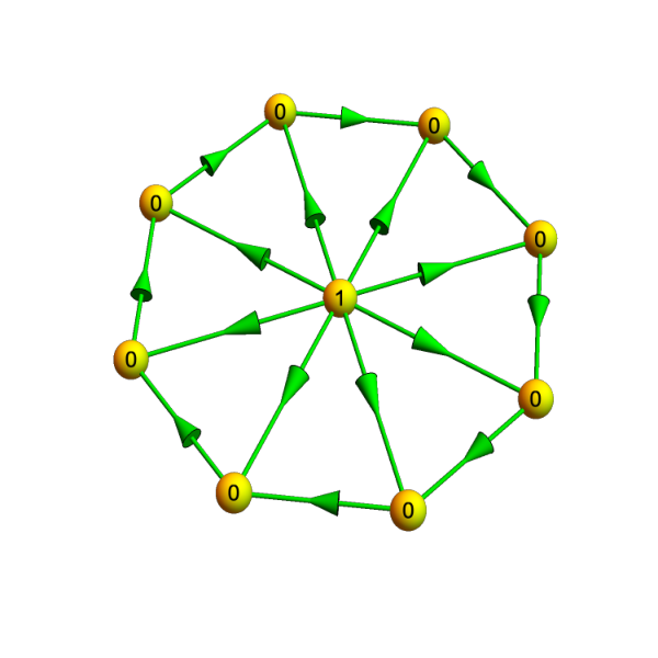
3) For $2$-graphs, graphs for which every unit sphere is a circular graph $C_{n}$ with $n\geq 4$, the index $i_{v}(x)$ is one minus the number of connectivity components of $S(x)$ which come into $x$. If all point into $x$ (this is a sink) or all point away from $x$ (this is a source), then the index is $1$. With exactly two components getting in and two parts getting out, we get a saddle. As in the continuum, the index can not get larger than $1$. The index is $0$ if there is one incoming direction and one outgoing direction.

In a broad way, curvature can be defined integral geometrically as index expectation. Gauss-Bonnet is then a direct consequence of Poincaré-Hopf, not requiring any proof. In the discrete, this has been explored in [8, 11, 10, 13]. The definition has the advantage that can be used as a definition both in the discrete as well as in the continuum. While indices are integers and so divisors, curvature $K$ is in general real-valued. It still satisfies the Gauss-Bonnet constraint, assuring that the total curvature is Euler characteristic.

We can so study the question which spaces allow for constant curvature and explore the first Hopf conjecture in the discrete: the later is the question whether positive sectional curvature implies positive Euler characteristic for even-dimensional discrete manifolds. Having the same question in the discrete allows a different avenue in exploring this notoriously difficult question for Riemannian manifolds. We will write about this oldest open problem in global differential geometry more elsewhere. Of course, positive curvature manifolds are then defined as a pair $(M,\mu)$ where the probability measure $\mu$ on Morse functions $\Omega$ has the property that for any point $x\in M$ and any any two dimensional plane in $T_{x}M$, the manifold $N=\exp_{x}(D)$ has positive $\mu$-curvature at $x$. This makes sense as almost all Morse functions on $M$ induce Morse functions on $N$ near $x$.

If $G=(V,E)$ is a finite simple graph. Assume that a probability measure $\mu$ on the space $\Omega$ of edge directions $F$ is given. This defines a probability measure $p_{x}$ on each simplex $x$. The probability $p_{x}(v)$ is the probability that $v$ is the largest element in $x$. The curvature $K(v)=E[i_{g}(v0]$ is the expectation of index functions $i_{g}(v)$. It satisfies

One interesting question we did not explore yet is how how big the probability of irrotational directed graphs are in the space of all directed Erdös-Rényi graphs with $n$ vertices and edge probability $p$ and how to construct irrotational directions more generally than using potentials $g:V\to\mathbb{R}$ and defining $v\to w$ if $g(v)<g(w)$. For $p=1$, we look at complete graphs of $n$ elements which has $m=n(n-1)/2$ edges and $2^{m}$ directions. We expect for each triangle to have a probability $6/2^{3}=3/4$ to produce no cycle of length $3$. As triangles appear with probability scaling $p^{3}$ and each triangle is with probability $1/4$ cyclic, we expect cyclic triangles to appear with a frequency with which triangles appear when the probability is $p\cdot(3/4)^{1/3}\sim 0.908p$.

Let $M$ be a smooth compact Riemannian manifold and let $\mu$ be a probability measure on smooth vector fields $F$ such that for $\mu$-almost all fields $F$, there are only finitely many hyperbolic equilibrium points. The later means that the Jacobean $dF(x)$ is invertible at every of the finitely many equilibrium point. We can then get a curvature on $M$ by taking the index expectation of these vector fields.

For example, if $\mu$ is a measure on the set of Morse functions $g$ of a Riemannian manifold $M$, then the Hessian at a critical point of a function $g$ is the Jacobean of $F={\rm grad}(g)$. The Morse condition assures that the Hessians are invertible. The index expectation $K$ satisfies automatically Gauss-Bonnet. Such measures always exist. Can every smooth function $K$ be realized as index expectation if the Euler characteristic constraint is satisfied? More precisely, given a smooth function $K$ on $M$ satisfying $\int_{M}K\;dV=\chi(G)$, is there a measure on Morse functions such that $K$ is the index expectation? What we can show so far is that on any Riemannian manifold $M$ there is a measure $\mu$ on Morse functions which produces a constant curvature $K$. This will be explored a bit elsewhere.

How do we get the Gauss-Bonnet-Chern integrand, the curvature $K$ which produces the Euler characteristic $\int_{M}K(x)\;dV(x)=\chi(M)$ as a Pfaffian of a Riemannian curvature tensor expression? One possibility is to Nash [17] embed the Riemannian manifold into a finite dimensional Euclidean space $E$ and to take the probability space $\Omega$ of linear functions on $E$ which is a finite dimensional manifold and carries a natural unique rotational invariant measure $\mu$. Almost every function $g$ is known to be Morse with respect to this measure. It defines so Poincaré-Hopf indices $i_{g}(x)$ for almost every $g$. This leads to a curvature $K(x)=E[i_{g}(x)]$ which satisfies the theoremum egregium (meaning that it is independent of the embedding). It also agrees with the Euler curvature:

The integral geometric point of view has been put forward earlier in [1]. The Regge approach allows to fit the discrete and continuum using integral geometry. The frame works of Poincaré-Hopf curvature works equally well for polytopes and manifolds and graphs.

An other approach is to define axiomatically what a “good curvature” on a Riemannian manifold should be. Let us assume that $M$ is a smooth, compact Riemannian manifold and say that $K$ is a “good curvature” if the following properties hold:

• •

  $K$ is a smooth function on $M$.

• •

  Generalizes Gauss: In the two dimensional case, $K$ is the Gauss curvature.

• •

  In odd dimensions, $K$ is identically zero.

• •

  Gauss-Bonnet: $\int_{M}K(x)\;dV(x)=\chi(M)$ is the Euler characteristic.

• •

  Theorema Egregium: $K$ does not depend on any embedding in an ambient space.

• •

  $K$ is local in the sense that $K(x)$ for $M$ is the same than the curvature of $K(x)$ when restricted to a small neighborhood of $x$.

Added December 21: One could add $K_{M\times N}(x,y)=K_{M}(x)K_{N}(x)$, if $M,N$ are two even dimensional manifolds.

We believe that in even dimensions, the Gauss-Bonnet-Chern integrand is the only choice for these postulates. Since also the index expectation of a probability space of linear functions in an ambient Euclidean space satisfies the postulates, this would establish the relation proven so far only via Regge calculus. Not everything with name curvature qualifies. Ricci curvature, sectional curvature, mean curvature or scalar curvatures are of different type. Already curvature $|T^{\prime}|/|r^{\prime}|$ with $T=|r^{\prime}|$ of a parametrization of a curve is an example of a curvature which does not qualify, even without the odd dimension assumption. It does not satisfy the Gauss-Bonnet formula for example.

A direct link between the continuum and discrete is given by internal set theory [18]. In that theory, a new attribute “standard” is added to the standard axioms ZFC of set theory using three axioms. The advantage of internal set theory to other non-standard approaches is that usual mathematics is untouched and that it is known to be a consistent extension of ZFC. A language extension allows for powerful shortcuts in real analysis and or probability theory. For the later see the astounding monograph [19]. Borrowing terminology of that book, one could name discrete graph theoretical approaches to Riemannian geometry a “radically elementary differential geometry”. It is extremely simple and works as follows:

In general for any mathematical object, there exists a finite set which contains all the standard elements in that object. (See Theorem 1.2 in [18]). In particular, given a compact manifold $M$, there exists a finite set $V$ which contains all standard points of $M$. This set is the vertex set of a graph. Let $\epsilon>0$ be any positive number we can say that two points in $M$ are called “connected” if their distance is smaller than $\epsilon$. Now define the edge set $E$ as the set of pairs $(x,y)$ such that $x$ and $y$ are connected. This defines a finite simple graph. It depends on $\epsilon$. (One can not define it without specifying some $\epsilon$ by using pairs which are infinitesimally close. The axiom (S) in the IST requires the relation $\phi$ to be internal. This is a classical mistake done when using non-standard analysis and it was done in the first version of this paper. Thanks to Michael Katz to point this error out to me). Here are the three axioms IST of Nelson which extend ZFC:

There are now Poincaré-Hopf or Gauss-Bonnet formulas available and they lead to the same results if $\epsilon$ is infinitesimal. The graph $(V,E)$ is naturally homotopic to any good triangulation of the manifold. It is of course of much larger dimension but we do not care. But the finite simple graph $(V,E)$ gives more, it contains all information about the original manifold $M$.

Can one recover the Riemannian metric? Not from the graph itself as homeomorphic manifolds can be modeled by graph isomorphic graphs. We need more structure. There are two ways to compute distances in the graph: use the Connes formula [3] from the Dirac operator $D=d+d^{*}$ defined by the exterior derivative $d$ defined on the graph has an advantage that it can be deformed [12]. An other is to define the distance between two points $x,y$ as the geodesic distance between two points in the graph and scale this so that the diameter of $G$ is the same than the diameter of the manifold. The measure $\mu$ on Morse functions which produces the Euler curvature however should allow to recover the distance as Crofton formulas allow to define a length of curves integral geometrically and so define a notion of geodesic.

The simplest curvature is the signed curvature $\frac{d}{dt}{\rm arg}(r^{\prime}(t))$ of a planar curve $r(t)$. Gauss-Bonnet in that case goes under the name Hopf Umlaufsatz which tells that for a simple closed $C^{2}$ curve, the total signed curvature is $2\pi$. We mention the Hopf proof [7] because the index expectation definition of curvature allows deformations. Since Hopf could handle a subtle case with elegance using deformation, there is an obvious question whether one can deform the measure $\mu$ defining curvature to make it positive if all sectional curvatures are positive. The Euler curvature has long been known not to be positive if curvature is positive.

Hopf proved this through a homotopy argument. Assume $r(t)$ is parametrized as $r:[0,1]\to\mathbb{R}^{2}$. Given a path from $(0,0)$ to $(1,1)$ he looked at the total angle change which must be a multiple of $2\pi$. As the total change depends continuously on the curve, homotopic curves from $(0,0)$ to $(1,1)$ have the same total change. Going from $(0,0)$ to $(1,0)$ gives $\pi$. Going from $(1,0)$ to $(1,1)$ again gives $\pi$. So that the piecewise linear path from $(0,0)$ to $(1,1)$ gives a change of $2\pi$.

In the case of a one dimensional manifold, maxima have index $-1$ and minima have index $1$. The Puiseux formula shows that the expectation value of the index is the signed curvature $K(t)=r^{\prime}(t)\times r^{\prime\prime}(t)/|r^{\prime}(t)|^{3}$. Gauss-Bonnet is then the Hopf Umlaufsatz. The Gauss-Bonnet-Chern integrand is a priori not defined in the odd-dimensional case but there is an integral geometric invariant.

References

- [1] T. Banchoff. Critical points and curvature for embedded polyhedra. J. Differential Geometry, 1:245–256, 1967.
- [2] J. Cheeger, W. Müller, and R. Schrader. On the curvature of piecewise flat spaces. Comm. Math. Phys, 92(3):405–454, 1984.
- [3] A. Connes. Noncommutative geometry. Academic Press, 1994.
- [4] K.S. Thorne C.W. Misner and J.A. Wheeler. Gravitation. Freeman, San Francisco, 1973.
- [5] H.L. Cycon, R.G.Froese, W.Kirsch, and B.Simon. Schrödinger Operators—with Application to Quantum Mechanics and Global Geometry. Springer-Verlag, 1987.
- [6] H. Hopf. Über die Curvatura integra geschlossener Hyperflaechen. Mathematische Annalen, 95:340–367, 1926.
- [7] H. Hopf. Über die Drehung der Tangenten und Sehnen ebener Curven. Compositio Math., 2, pages 50–62, 1935.
- [8]
O. Knill.
A graph theoretical Gauss-Bonnet-Chern theorem.
http://arxiv.org/abs/1111.5395, 2011. - [9]
A graph theoretical Poincaré-Hopf theorem.
http://arxiv.org/abs/1201.1162, 2012. - [10]
An index formula for simple graphs .
http://arxiv.org/abs/1205.0306, 2012. - [11]
On index expectation and curvature for networks.
http://arxiv.org/abs/1202.4514, 2012. - [12]
The Dirac operator of a graph.
http://http://arxiv.org/abs/1306.2166, 2013. - [13]
The Euler characteristic of an even-dimensional graph.
http://arxiv.org/abs/1307.3809, 2013. - [14]
Dehn-Sommerville from Gauss-Bonnet.
https://arxiv.org/abs/1905.04831, 2019. - [15]
A parametrized Poincare-Hopf theorem and clique cardinalities of
graphs.
https://arxiv.org/abs/1906.06611, 2019. - [16]
Poincaré-hopf for vector fields on graphs.
https://arxiv.org/abs/1911.04208, 2019. - [17] Harold W. Kuhn and Sylvia Nasar. The Essential Nash. Princeton University Press, 2002.
- [18] E. Nelson. Internal set theory: A new approach to nonstandard analysis. Bull. Amer. Math. Soc, 83:1165–1198, 1977.
- [19] E. Nelson. Radically elementary probability theory. Princeton university text, 1987.
- [20] H. Poincaré. Sur les courbes definies par les equation differentielle III. Journal de Mathematique pures et appliquées, pages 167–244, 1885.
- [21] T. Regge. General relativity without coordinates. Nuovo Cimento (10), 19:558–571, 1961.
- [22] M. Spivak. A comprehensive Introduction to Differential Geometry I-V. Publish or Perish, Inc, Berkeley, third edition, 1999.