Constant-roll -Inflation Dynamics
Abstract
In this work we shall investigate the phenomenological implications of the constant-roll condition on a -Inflation theory of gravity. The latter theories are particularly promising, since these remained robust to the results of GW170817, since these have a gravitational wave speed in natural units. We shall mainly focus on the phenomenology of the -Inflation models, with the only assumption being the slow-roll condition imposed on the first and fourth slow-roll parameters, and the constant-roll condition for the evolution of the scalar field. We present in detail the final form of the gravitational equations of motion that control the dynamics of the cosmological system, with the constant-roll condition imposed, and by using a conveniently, from the perspective of analytical manipulations, chosen potential, we express the slow-roll indices and the resulting observational indices of the theory as functions of the -foldings number. The results of our analysis indicate that the constant-roll -Inflation theory can be compatible with the Planck 2018 data, for a wide range of the free parameters. Also we examine in a quantitative way the effects of the constant-roll condition on the parameter on which the bispectrum is proportional, in the equilateral momentum approximation, and we demonstrate that the effect of the constant-roll condition is non-trivial. In effect, non-Gaussianities in the theory may be enhanced, a phenomenon which is known to be produced by constant-roll scalar theories of gravity in general.
pacs
04.50.Kd, 95.36.+x, 98.80.-k, 98.80.Cq,11.25.-wI Introduction
One of the prominent problems in modern theoretical cosmology is to describe accurately the primordial era of our Universe, and particularly the inflationary era, during which our Universe expanded in a nearly exponential rate and became homogenized. To this problem, continuous efforts focusing on the Cosmic Microwave Background structure and inhomogeneity, lead to astonishing results that constrain quite strongly the inflationary spectrum to great accuracy Akrami:2018odb. Particularly, the power spectrum of the scalar primordial curvature perturbations seems to be nearly scale invariant and the tensor-to-scalar ratio is small of the order . Initially, inflationary theories were materialized in terms of a scalar field, the inflaton, which controlled the evolution of the Universe during the rapid primordial accelerating era Guth:1980zm; Starobinsky:1982ee; Linde:1983gd; Albrecht:1982wi, however nowadays modified gravity also provides a consistent theoretical framework that can harbor the inflationary era, for reviews see Nojiri:2017ncd; Nojiri:2010wj; Nojiri:2006ri; Capozziello:2011et; Capozziello:2010zz; delaCruzDombriz:2012xy; Olmo:2011uz. The Planck satellite observational data severely constrained the inflationary era, and narrowed down to a great extent the viable inflationary scenarios, leaving only a few scalar theories of inflation intact with regards their viability. However, many modified gravity models still remain quite viable and compatible with the Planck predictions Akrami:2018odb.
In 2017, the GW170817 event GBM:2017lvd further constrained the inflationary theories, due to the fact that the gravitational waves and the electromagnetic signal emitted from the merging of the two neutron stars came simultaneously. This indicated that the gravitational wave speed was in natural units, thus this phenomenal event eliminated many theoretical models of inflation, like most of the Horndeski theories, and many of the string corrected models involving couplings of the scalar field to the Gauss-Bonnet invariant, see Ref. Ezquiaga:2017ekz for details on the currently allowed theories. One of the surviving theories are the so-called -Inflation theories ArmendarizPicon:1999rj; Chiba:1999ka; ArmendarizPicon:2000dh; Matsumoto:2010uv; ArmendarizPicon:2000ah; Chiba:2002mw; Malquarti:2003nn; Malquarti:2003hn; Chimento:2003zf; Chimento:2003ta; Scherrer:2004au; Aguirregabiria:2004te; ArmendarizPicon:2005nz; Abramo:2005be; Rendall:2005fv; Bruneton:2006gf; dePutter:2007ny; Babichev:2007dw; Deffayet:2011gz; Kan:2018odq; Unnikrishnan:2012zu; Li:2012vta which have also the appealing feature of being able to describe the dark energy era too.
In this paper we shall investigate the phenomenological features of -Inflation theories by assuming that the constant-roll condition Inoue:2001zt; Tsamis:2003px; Kinney:2005vj; Tzirakis:2007bf; Namjoo:2012aa; Martin:2012pe; Motohashi:2014ppa; Cai:2016ngx; Motohashi:2017aob; Hirano:2016gmv; Anguelova:2015dgt; Cook:2015hma; Kumar:2015mfa; Odintsov:2017yud; Odintsov:2017qpp; Lin:2015fqa; Gao:2017uja; Nojiri:2017qvx; Oikonomou:2017bjx; Odintsov:2017hbk; Oikonomou:2017xik; Cicciarella:2017nls; Awad:2017ign; Anguelova:2017djf; Ito:2017bnn; Karam:2017rpw; Yi:2017mxs; Mohammadi:2018oku; Gao:2018tdb; Mohammadi:2018wfk; Morse:2018kda; Cruces:2018cvq; GalvezGhersi:2018haa; Boisseau:2018rgy; Gao:2019sbz; Lin:2019fcz holds true. The astonishing feature of the constant-roll condition, is that it is associated with primordial non-Gaussianities in the power spectrum of the CMB Liddle:2000cg. In ordinary -Inflation theories, if the slow-roll assumption is taken into account, the non-Gaussianities are expected to be small DeFelice:2011zh, however the constant-roll condition may enhance the non-Gaussianities in the bispectrum, in the equilateral momentum approximation. Our purpose is to present the formalism of -Inflation theories in the constant-roll approximation in detail, and calculate the spectral index of the scalar primordial curvature perturbations and the tensor-to-scalar ratio. In addition, we shall investigate for certain models the factor that appears in the bispectrum, in the equilateral momentum approximation. The -Inflation theories are theories of the general form , with , the perturbations of which were studied in detail in Refs. Noh:2001ia; Hwang:2005hb; Hwang:2002fp; Kaiser:2013sna. Our aim is to present the general form of the “slow-roll” indices capturing the inflationary dynamics in the constant-roll approximation, and investigate whether these theories can provide a viable phenomenology, compatible with the latest Planck data Akrami:2018odb. In addition, we shall examine the possibility whether the bispectrum can be enhanced by the constant-roll condition. For the moment, the Gaussian structure of the primordial scalar models of the perturbations is not questioned, but future observations may distort the Gaussianity assumption, so this paper aims to introduce a theoretical description that may survive from the Planck, GW170817 and from future observations that may indicate the presence of non-Gaussianities in the power spectrum of the primordial scalar perturbations modes. Apart from this fact which clearly motivates the use of the constant-roll condition, we need to explain the motivation for using a -inflation theory to study its phenomenological aspects. The motivation comes from the fact that the -inflation theory is the most general theory that can describe inflation with a single scalar field in the context of Einstein gravity Lyth:2009zz. Apart from this, the GW170817 result significantly narrowed down the possible theories that may consistently describe gravitational interactions, thus the remaining viable theories must in some way studied in further detail in order to reveal all the possible phenomenological implications of these.
Our study will be focused on flat background geometries, and specifically we shall assume that the background geometry is that of a flat Friedman-Robertson-Walker (FRW), with line element,
| (1) |
where is the scale factor.
II Constant-roll -Inflation Gravity: Equations of Motion and Inflationary Dynamics
The -Inflation model we shall consider, belongs to the general class of theories, with gravitational action,
| (2) |
where in our case, the function which we shall consider is equal to,
| (3) |
In Eq. (3), , is the scalar potential, is a real number which will be assumed to be equal to , with this value corresponding to a canonical scalar field, however we keep the notation for general because in this way if one wants to study the phantom scalar case, which corresponds to , one just have to replace in the resulting equations. Finally, , where is the reduced Planck mass, and is a free parameter of mass units . For the FRW background (1), the gravitational equations of motion become,
| (4) |
| (5) |
| (6) |
where the “dot” indicates differentiation with respect to the cosmic time, and . Using the functional form of the function (3), the gravitational equations become,
| (7) |
| (8) |
| (9) |
and note that in our case. The dynamical evolution of the cosmological system is controlled by the differential equations (7), (8), (9), given the potential , however solving these analytically is a formidable task, unless some simplification is implied. We shall quantify the dynamics of inflation in terms of the “slow-roll” parameters Hwang:2005hb (which are traditionally called like this, without assuming for the moment that these are small numbers),
| (10) |
where in our case is,
| (11) |
Note here that we used a different definition of the slow-roll in comparison to the standard one Stewart:1993bc; Habib:2002yi. Hereafter we impose the slow-roll condition, only on the slow-roll parameters and , so during the inflationary era, and also we assume that . However, these assumptions-constraints must be checked if they hold true. The slow-roll condition only on is necessary in order to ensure an exit from the inflationary era, when this slow-roll parameter becomes of the order . In addition, we shall assume that the constant-roll condition holds true, which is,
| (12) |
where is some dimensionless real parameter of the order , so the constant-roll condition affects practically the “slow-roll” parameter which is required to be .
For the FRW metric, assuming that the scalar field depends solely on the cosmic time, becomes , and by substituting this in Eqs. (7), (8), (9), in conjunction with the constant-roll condition (12), the gravitational equations of motion become,
| (13) |
| (14) |
| (15) |
By taking into account the assumption , the first two gravitational equations become more simple,
| (16) |
| (17) |
From Eq. (15) it is apparent that the -Inflation contribution to the inflationary evolution comes from terms .
Let us discuss certain features of Eq. (15). It is apparently a third order equation with respect to , so it has three solutions, two of which are complex and thus not physically interesting, thus we shall use the one with real values of . An important comment is in order, notice that if we take the limit and in Eq. (15), we obtain,
| (18) |
which is the slow-roll solution. If however one solves algebraically Eq. (15), the limit and cannot be taken in the solution, so the slow-roll solution cannot be obtained from the solutions of Eq. (15) by taking the limit and . Mathematically this is easy to understand, since Eq. (15) describes a curve with non-zero curvature as a function of , so the roots of Eq. (15) are the points where this curve meets the axis. The slow-roll solution describes a straight line, instead of a non-zero curvature curve in the plane. To see this more explicitly consider the curve,
| (19) |
with , and being real parameters. The above equation has three solutions, two of which are complex conjugate so we do not quote here, but the real solution is,
| (20) |
As it can be seen, we cannot take the limit , infinities occur, but this limit can be taken for the algebraic equation (19), yielding . Let us return to the problem at hand, so by solving the algebraic equation (15) with respect to , we obtain the following real solution,
| (21) |
and by substituting this to Eq. (12) in conjunction with Eq. (16) we get,
| (22) |
where and in both Eqs. (21) and (22) are defined as follows,
| (23) |
| (24) |
We also have the wave speed which characterizes the propagation of the primordial perturbations, for the -Inflation theory, which will be needed for the calculation of the tensor-to-scalar ratio,
| (25) |
while the gravitational wave speed is , which is why the -Inflation theories are still compatible with the GW170817 event.
Let us proceed to give the expressions of the “slow-roll” indices for the theory at hand, having in mind that these must be evaluated at the horizon crossing time instance, where the value of the scalar field is . After some simple calculations and by combining Eqs. (10), (11), (16) and (17), these are equal to,
| (26) | ||||
where and are functions of the scalar field , as in Eqs. (21) and (22). Accordingly, the spectral index of the primordial curvature perturbations is equal to Hwang:2005hb,
| (27) |
which holds true even in the case that the do not take small values. In addition, the analytic form of the tensor-to-scalar ratio is for the theory at hand Hwang:2005hb,
| (28) |
which must be evaluated at the horizon crossing. For the above calculation we assumed that the slow-roll indices and take small values during the inflationary era, a condition which we must check if it holds true at the end of this section. Notice that for the slow-roll case, the tensor-to-scalar ratio is , so the constant-roll and -Inflation effects are materialized in the parameters and in Eq. (28). Having the slow-roll indices as functions of the scalar field, now we can proceed in expressing those as functions of the -foldings number , which is defined as follows,
| (29) |
where is the time instance that inflation starts, which we shall assume it to be equal to the time instance of horizon crossing, at which , while is the time instance that inflation ends. Of course inflation is known to start quite earlier than the horizon crossing time instance, but we choose to be the horizon crossing time instance, because the condition is vital for the calculation of the power spectrum, both scalar and tensor. Also we need to note that the initial condition of the constant-roll -inflation theory may be a Bunch-Davies vacuum state Oikonomou:2017isf or a quasi-de Sitter like expansion which leads to a Bunch-Davies vacuum state Keskin:2018gev. Expressed in terms of the scalar field, the -foldings number is equal to,
| (30) |
or by using Eq. (16), this can be written as,
| (31) |
which in view of Eq. (21) yields the -foldings number as a function of the scalar field . The value of the scalar field at the end of the inflationary era can be evaluated easily, since at that era, , so is obtained. Thus by substituting the result in Eq. (31) and performing the -integration, one can have as a function of the -foldings number. In effect, the slow-roll indices (26) and the corresponding observational indices (27) and (28) can be expressed as functions of the -foldings number, and a direct confrontation with the observational data can be done. In the next section we shall examine some specific examples of potentials, in order to see whether a viable phenomenology can be obtained from the constant-roll -Inflation theory.
II.1 Inflationary Phenomenology of Constant-roll -Inflation Power-law Scalar Potentials
In the previous subsection we developed the formalism for the inflationary dynamics of constant-roll -Inflation theory, and in this section we shall employ it in order to investigate the phenomenology of power-law potentials. However, the most serious setback is the lack of analyticity, so let us choose a relatively simple power-law potential,
| (32) |
where is some positive parameter with mass dimensions . For this potential, it is easy to obtain the Hubble rate and as functions of in closed form, however, in order to find analytically the value of the scalar field at the end of inflation and eventually to express the value of the scalar field at horizon crossing as a function of the -foldings number , we shall assume that the term is much larger than , that is,
| (33) |
with both the terms appearing in the function in Eq. (21), a condition that can be achieved if . Let us note here that the condition (33) is not related to the condition . However, we impose the condition (33) in order to make the analytic treatment easier, and we need to check after we present the phenomenology of the model, whether this holds true for the values of the free parameters that guarantee the phenomenological viability of the model.
Hereafter we choose reduced Planck units, in which , so the only assumption we shall make regarding the free parameters is that in Planck units. Having these assumptions in mind, can be evaluated in a simplified way and it is equal to,
| (34) |
Also, the value of the scalar field at the end of inflation can be evaluated by taking appearing in Eq. (26) to be equal to , so by combining Eqs. (34) and (32), we obtain the approximate solution,
| (35) |
and notice that in the end we must take in reduced Planck units. With , and the potential given, we can combine these and substitute their value in Eq. (31) in order to express the value of the scalar field at horizon crossing as a function of the -foldings number, and by doing so we obtain,
| (36) |
Having the above at hand, we can express the slow-roll indices (26) and the corresponding observational indices (27) and (28), as functions of the -foldings number, and we can consequently confront the theory with the observational data. The 2018 Planck data Akrami:2018odb constrain the spectral index and the tensor-to-scalar ratio as follows,
| (37) |
so let us investigate the phenomenology of the constant-roll -Inflation model. The resulting expressions for the observational indices are quite large to quote these here, but we shall quote the results of our analysis.
The compatibility of the resulting theory with the observational data can be achieved only for small values of the parameter and actually, the parameter crucially affects the viability of the model. Particularly, it seems that strongly alters the phenomenology of the model and the rest of the parameters have marginal effects, apart from the parameter which strongly affects the tensor-to-scalar ratio. For example for , in reduced Planck units, and for , and , we get the following values for the observational indices,
| (38) |
which are compatible with the latest Planck data (37). Recall that the 2018 Planck data (37) indicate that the spectral index should be in the range , so clearly the results (38) are within the allowed range. In addition, by choosing for example, , in reduced Planck units, and for , and , we get the following values for the observational indices,
| (39) |
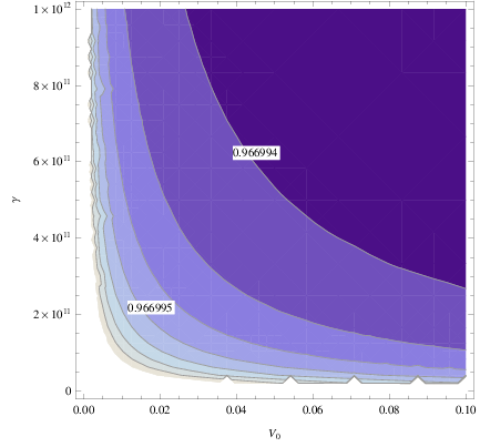
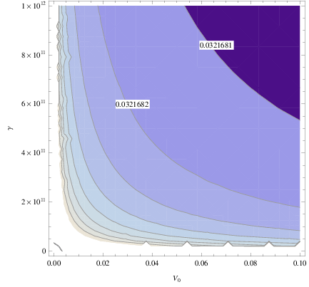
so it is obvious that , and do not affect the spectral index, however, the tensor-to-scalar ratio is strongly affected by the parameter . Indeed, if we choose , in reduced Planck units, and for , , as in the previous case, and choose additionally , the tensor-to-scalar ratio drops drastically to . So it seems that only the parameters and have a strong effect on the observational indices. In order to better illustrate this issue, in Fig. 1 we present the contour plots of the spectral index (left plot) and of the tensor-to-scalar ratio (right plot) as functions of and , for , and for chosen in the range and . In both the plots it is apparent that and do not crucially affect the observational indices. In both the plots, the lighter colors indicate larger values of the plotted quantities, and darker colors indicate smaller values of the respective plotted quantity. In both plots we indicated some characteristic values of the respective plotted quantity.
Before closing it is worth discussing another important issue, related with the values of the parameter which can be related with Jeans instabilities if or it may have superluminal values Babichev:2007dw. In our case, the results are free from superluminal velocities and Jeans instabilities, since defined in Eq. (25) takes values for a large range of the values of the free parameters chosen in such a way so that the observational indices are compatible with the observational data. For example, if we choose, , in reduced Planck units, and for and , we get,
| (40) |
In order to better understand the behavior of the velocity , in Fig. 2 we present the contour plots of as a function of and .
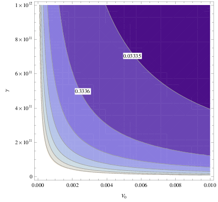
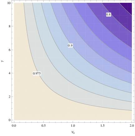
As it can be seen from both plots of Fig. 2, the sound wave speed hardly changes as and take different values. Furthermore, it can be shown that and also do not drastically affect the sound wave speed , and in all cases, the wave speed takes positive values with . In this case too, darker colors indicate larger values of the wave speed , and in both plots we indicated some characteristic values.
It is important to validate that the assumption we made in order to calculate the tensor-to-scalar ratio, holds true, for the allowed values of the free parameters of the model. Indeed, it can be checked that both , and take small values for the allowed values of the free parameters, for example by choosing , in reduced Planck units, and for , and , we have,
| (41) |
which are indeed quite smaller than unity. For these indices, the same rules apply, so these are crucially affected by the parameter .
Finally, it is also vital for the self-consistency of the model and the results presented above, to check whether the condition (33) holds true for the values of the free parameters that guarantee the phenomenological viability of the model. By choosing for example, , in reduced Planck units, and for , and , we have,
| (42) |
and
| (43) |
in reduced Planck units, which clearly indicates that the imposed condition (33) holds true.
II.2 The non-Gaussianities Issue
The primordial power spectrum of the curvature perturbations seems up to date to be Gaussian, to a high accuracy. However, the future observations may reveal non-Gaussianities in the spectrum, and these are quantified in the bispectrum and trispectrum, which in turn are quantified in the correlation functions and Lyth:2009zz. The momenta have to add up to zero, while the function is the bispectrum and is called the trispectrum. The constant-roll condition is known to produce non-Gaussianities in canonical single scalar field theory, so one of the purposes of this paper is to investigate whether this is possible in the context of constant-roll -Inflation theory. The calculation for the bispectrum in classes of theories were performed in several works, but in Ref. DeFelice:2011zh the bispectrum was calculated without assuming the slow-roll conditions on the slow-roll indices, so the result fits in an optimal way our work, because in our case the second slow-roll index does not take small values. We shall change the notation of Ref. DeFelice:2011zh in order to comply with the previous sections of our work, so in the equilateral momentum approximation, the parameter in terms of the slow-roll indices reads,
| (44) |
where the parameters and are defined as follows,
| (45) | ||||
and is defined in Eq. (25), while the parameters appearing in Eq. (45) are defined as follows,
| (46) |
Finally appearing in Eq. (46) is defined as follows,
| (47) |
By inserting the ’s and the ’s in Eq. (44), the parameter reads,
| (48) |
Finally, the parameters and were introduced for notational convenience, and these are defined as follows,
| (49) |
In order to have a concrete idea on the new effects that the constant-roll condition brings along in the -Inflation theory, let us use the numerical values of the free parameters for which we achieved the compatibility with the observational data, and let us compare the results with the slow-roll case. Obviously, the non-Gaussianity will be enhanced by the presence of the term , since . So for , we have, . This can be compared to the term which for is approximately , which is nearly one order smaller in comparison to the term . The result is still small, but more enhanced in comparison to the slow-roll case, and also it is within the acceptable limits of the 2018 Planck constraints on primordial non-Gaussianities, which indicate that Akrami:2019izv.
Thus the constant-roll condition may enhance the non-Gaussianities in the power spectrum of primordial curvature perturbations of the -Inflation theory with power-law potential. In principle, more phenomenologically interesting potentials can be used, but the lack of analyticity restricted us to use the simplest choices.
III Conclusions
In this paper we investigated the phenomenological implications of the constant-roll condition in a -Inflation theory in the presence of scalar potential. We presented in detail the structure of the gravitational equations of motion, in view of the constant-roll condition, and by assuming that only the first slow-roll index takes small values, thus quantifying the slow-roll condition only on this index, we formed the set of differential equations that governs the constant-roll -Inflation theory. By choosing a convenient potential, that may allow analytical manipulation of the equations to some extend, we expressed the slow-roll indices and the corresponding observational indices as functions of the -foldings number. As we demonstrated, the observational indices of the resulting quadratic potential theory can be compatible with the observational data coming from the latest Planck 2018 collaboration. Also we examined in some detail the quantitative effects of the constant-roll condition on the parameter appearing in the bispectrum, in the equilateral momentum approximation, and we demonstrated that non-trivial effects occur, thus non-Gaussianities are enhanced. In general, theories of -Inflation type, and generalizations, are particularly useful for providing theoretical descriptions both compatible with the Planck data on inflation and more importantly with the striking GW170817 event. Work is in progress towards a unified modified gravity -Inflation theory with general scalar potentials.
Finally we need to stress one more the fact that -inflation theories lead to a gravitational wave speed in natural units Hwang:2005hb, regardless of the values of the free parameters of the theory. This was partially the motivation for studying this specific class of theory with regard to its phenomenological implications.
Acknowledgments
This work is supported by MINECO (Spain), FIS2016-76363-P, and by project 2017 SGR247 (AGAUR, Catalonia) (S.D.O). SDO is grateful to Yi-Fu Cai for kind hospitality at USTC. This work is supported by the DAAD program “Hochschulpartnerschaften mit Griechenland 2016” (Projekt 57340132) (V.K.O). V.K.O is indebted to Prof. K. Kokkotas for his hospitality in the IAAT, University of Tübingen.
References
- (1) Y. Akrami et al. [Planck Collaboration], arXiv:1807.06211 [astro-ph.CO].
- (2) A. H. Guth, Phys. Rev. D 23 (1981) 347. doi:10.1103/PhysRevD.23.347
- (3) A. A. Starobinsky, Phys. Lett. 91B (1980) 99. doi:10.1016/0370-2693(80)90670-X
- (4) A. D. Linde, Phys. Lett. 129B (1983) 177. doi:10.1016/0370-2693(83)90837-7
- (5) A. Albrecht and P. J. Steinhardt, Phys. Rev. Lett. 48 (1982) 1220 [Adv. Ser. Astrophys. Cosmol. 3 (1987) 158]. doi:10.1103/PhysRevLett.48.1220
- (6) S. Nojiri, S. D. Odintsov and V. K. Oikonomou, Phys. Rept. 692 (2017) 1 doi:10.1016/j.physrep.2017.06.001 [arXiv:1705.11098 [gr-qc]].
- (7) S. Nojiri and S. D. Odintsov, Phys. Rept. 505 (2011) 59 doi:10.1016/j.physrep.2011.04.001 [arXiv:1011.0544 [gr-qc]].
- (8) S. Nojiri and S. D. Odintsov, eConf C 0602061 (2006) 06 [Int. J. Geom. Meth. Mod. Phys. 4 (2007) 115] doi:10.1142/S0219887807001928 [hep-th/0601213].
- (9) S. Capozziello and M. De Laurentis, Phys. Rept. 509 (2011) 167 doi:10.1016/j.physrep.2011.09.003 [arXiv:1108.6266 [gr-qc]].
- (10) V. Faraoni and S. Capozziello, Fundam. Theor. Phys. 170 (2010). doi:10.1007/978-94-007-0165-6
- (11) A. de la Cruz-Dombriz and D. Saez-Gomez, Entropy 14 (2012) 1717 doi:10.3390/e14091717 [arXiv:1207.2663 [gr-qc]].
- (12) G. J. Olmo, Int. J. Mod. Phys. D 20 (2011) 413 doi:10.1142/S0218271811018925 [arXiv:1101.3864 [gr-qc]].
- (13) B. P. Abbott et al. “Multi-messenger Observations of a Binary Neutron Star Merger,” Astrophys. J. 848 (2017) no.2, L12 doi:10.3847/2041-8213/aa91c9 [arXiv:1710.05833 [astro-ph.HE]].
- (14) J. M. Ezquiaga and M. Zumalacarregui, Phys. Rev. Lett. 119 (2017) no.25, 251304 doi:10.1103/PhysRevLett.119.251304 [arXiv:1710.05901 [astro-ph.CO]].
- (15) C. Armendariz-Picon, T. Damour and V. F. Mukhanov, Phys. Lett. B 458 (1999) 209 doi:10.1016/S0370-2693(99)00603-6 [hep-th/9904075].
- (16) T. Chiba, T. Okabe and M. Yamaguchi, Phys. Rev. D 62 (2000) 023511 doi:10.1103/PhysRevD.62.023511 [astro-ph/9912463].
- (17) C. Armendariz-Picon, V. F. Mukhanov and P. J. Steinhardt, Phys. Rev. Lett. 85 (2000) 4438 doi:10.1103/PhysRevLett.85.4438 [astro-ph/0004134].
- (18) J. Matsumoto and S. Nojiri, Phys. Lett. B 687 (2010) 236 doi:10.1016/j.physletb.2010.03.030 [arXiv:1001.0220 [hep-th]].
- (19) C. Armendariz-Picon, V. F. Mukhanov and P. J. Steinhardt, Phys. Rev. D 63 (2001) 103510 doi:10.1103/PhysRevD.63.103510 [astro-ph/0006373].
- (20) T. Chiba, Phys. Rev. D 66 (2002) 063514 doi:10.1103/PhysRevD.66.063514 [astro-ph/0206298].
- (21) M. Malquarti, E. J. Copeland, A. R. Liddle and M. Trodden, Phys. Rev. D 67 (2003) 123503 doi:10.1103/PhysRevD.67.123503 [astro-ph/0302279].
- (22) M. Malquarti, E. J. Copeland and A. R. Liddle, Phys. Rev. D 68 (2003) 023512 doi:10.1103/PhysRevD.68.023512 [astro-ph/0304277].
- (23) L. P. Chimento and A. Feinstein, Mod. Phys. Lett. A 19 (2004) 761 doi:10.1142/S0217732304013507 [astro-ph/0305007].
- (24) L. P. Chimento, Phys. Rev. D 69 (2004) 123517 doi:10.1103/PhysRevD.69.123517 [astro-ph/0311613].
- (25) R. J. Scherrer, Phys. Rev. Lett. 93 (2004) 011301 doi:10.1103/PhysRevLett.93.011301 [astro-ph/0402316].
- (26) J. M. Aguirregabiria, L. P. Chimento and R. Lazkoz, Phys. Rev. D 70 (2004) 023509 doi:10.1103/PhysRevD.70.023509 [astro-ph/0403157].
- (27) C. Armendariz-Picon and E. A. Lim, JCAP 0508 (2005) 007 doi:10.1088/1475-7516/2005/08/007 [astro-ph/0505207].
- (28) L. R. Abramo and N. Pinto-Neto, Phys. Rev. D 73 (2006) 063522 doi:10.1103/PhysRevD.73.063522 [astro-ph/0511562].
- (29) A. D. Rendall, Class. Quant. Grav. 23 (2006) 1557 doi:10.1088/0264-9381/23/5/008 [gr-qc/0511158].
- (30) J. P. Bruneton, Phys. Rev. D 75 (2007) 085013 doi:10.1103/PhysRevD.75.085013 [gr-qc/0607055].
- (31) R. de Putter and E. V. Linder, Astropart. Phys. 28 (2007) 263 doi:10.1016/j.astropartphys.2007.05.011 [arXiv:0705.0400 [astro-ph]].
- (32) E. Babichev, V. Mukhanov and A. Vikman, JHEP 0802 (2008) 101 doi:10.1088/1126-6708/2008/02/101 [arXiv:0708.0561 [hep-th]].
- (33) C. Deffayet, X. Gao, D. A. Steer and G. Zahariade, Phys. Rev. D 84 (2011) 064039 doi:10.1103/PhysRevD.84.064039 [arXiv:1103.3260 [hep-th]].
- (34) N. Kan, K. Shiraishi and M. Yashiki, arXiv:1811.11967 [gr-qc].
- (35) S. Unnikrishnan, V. Sahni and A. Toporensky, JCAP 1208 (2012) 018 doi:10.1088/1475-7516/2012/08/018 [arXiv:1205.0786 [astro-ph.CO]].
- (36) S. Li and A. R. Liddle, JCAP 1210 (2012) 011 doi:10.1088/1475-7516/2012/10/011 [arXiv:1204.6214 [astro-ph.CO]].
- (37) S. Inoue and J. Yokoyama, Phys. Lett. B 524 (2002) 15 doi:10.1016/S0370-2693(01)01369-7 [hep-ph/0104083].
- (38) N. C. Tsamis and R. P. Woodard, Phys. Rev. D 69 (2004) 084005 doi:10.1103/PhysRevD.69.084005 [astro-ph/0307463].
- (39) W. H. Kinney, Phys. Rev. D 72 (2005) 023515 doi:10.1103/PhysRevD.72.023515 [gr-qc/0503017].
- (40) K. Tzirakis and W. H. Kinney, Phys. Rev. D 75 (2007) 123510 doi:10.1103/PhysRevD.75.123510 [astro-ph/0701432].
- (41) M. H. Namjoo, H. Firouzjahi and M. Sasaki, Europhys. Lett. 101 (2013) 39001 doi:10.1209/0295-5075/101/39001 [arXiv:1210.3692 [astro-ph.CO]].
- (42) J. Martin, H. Motohashi and T. Suyama, Phys. Rev. D 87 (2013) no.2, 023514 doi:10.1103/PhysRevD.87.023514 [arXiv:1211.0083 [astro-ph.CO]].
- (43) H. Motohashi, A. A. Starobinsky and J. Yokoyama, JCAP 1509 (2015) no.09, 018 doi:10.1088/1475-7516/2015/09/018 [arXiv:1411.5021 [astro-ph.CO]].
- (44) Y. F. Cai, J. O. Gong, D. G. Wang and Z. Wang, JCAP 1610 (2016) no.10, 017 doi:10.1088/1475-7516/2016/10/017 [arXiv:1607.07872 [astro-ph.CO]].
- (45) H. Motohashi and A. A. Starobinsky, arXiv:1702.05847 [astro-ph.CO].
- (46) S. Hirano, T. Kobayashi and S. Yokoyama, Phys. Rev. D 94 (2016) no.10, 103515 doi:10.1103/PhysRevD.94.103515 [arXiv:1604.00141 [astro-ph.CO]].
- (47) L. Anguelova, Nucl. Phys. B 911 (2016) 480 doi:10.1016/j.nuclphysb.2016.08.020 [arXiv:1512.08556 [hep-th]].
- (48) J. L. Cook and L. M. Krauss, JCAP 1603 (2016) no.03, 028 doi:10.1088/1475-7516/2016/03/028 [arXiv:1508.03647 [astro-ph.CO]].
- (49) K. S. Kumar, J. Marto, P. Vargas Moniz and S. Das, JCAP 1604 (2016) no.04, 005 doi:10.1088/1475-7516/2016/04/005 [arXiv:1506.05366 [gr-qc]].
- (50) S. D. Odintsov and V. K. Oikonomou, arXiv:1703.02853 [gr-qc].
- (51) S. D. Odintsov and V. K. Oikonomou, arXiv:1704.02931 [gr-qc].
- (52) J. Lin, Q. Gao and Y. Gong, Mon. Not. Roy. Astron. Soc. 459 (2016) no.4, 4029 doi:10.1093/mnras/stw915 [arXiv:1508.07145 [gr-qc]].
- (53) Q. Gao and Y. Gong, arXiv:1703.02220 [gr-qc].
- (54) S. Nojiri, S. D. Odintsov and V. K. Oikonomou, Class. Quant. Grav. 34 (2017) no.24, 245012 doi:10.1088/1361-6382/aa92a4 [arXiv:1704.05945 [gr-qc]].
- (55) V. K. Oikonomou, Mod. Phys. Lett. A 32 (2017) no.33, 1750172 doi:10.1142/S0217732317501723 [arXiv:1706.00507 [gr-qc]].
- (56) S. D. Odintsov, V. K. Oikonomou and L. Sebastiani, Nucl. Phys. B 923 (2017) 608 doi:10.1016/j.nuclphysb.2017.08.018 [arXiv:1708.08346 [gr-qc]].
- (57) V. K. Oikonomou, Int. J. Mod. Phys. D 27 (2017) no.02, 1850009 doi:10.1142/S0218271818500098 [arXiv:1709.02986 [gr-qc]].
- (58) F. Cicciarella, J. Mabillard and M. Pieroni, JCAP 1801 (2018) no.01, 024 doi:10.1088/1475-7516/2018/01/024 [arXiv:1709.03527 [astro-ph.CO]].
- (59) A. Awad, W. El Hanafy, G. G. L. Nashed, S. D. Odintsov and V. K. Oikonomou, JCAP 1807 (2018) no.07, 026 doi:10.1088/1475-7516/2018/07/026 [arXiv:1710.00682 [gr-qc]].
- (60) L. Anguelova, P. Suranyi and L. C. R. Wijewardhana, JCAP 1802 (2018) no.02, 004 doi:10.1088/1475-7516/2018/02/004 [arXiv:1710.06989 [hep-th]].
- (61) A. Ito and J. Soda, Eur. Phys. J. C 78 (2018) no.1, 55 doi:10.1140/epjc/s10052-018-5534-5 [arXiv:1710.09701 [hep-th]].
- (62) A. Karam, L. Marzola, T. Pappas, A. Racioppi and K. Tamvakis, JCAP 1805 (2018) no.05, 011 doi:10.1088/1475-7516/2018/05/011 [arXiv:1711.09861 [astro-ph.CO]].
- (63) Z. Yi and Y. Gong, JCAP 1803 (2018) no.03, 052 doi:10.1088/1475-7516/2018/03/052 [arXiv:1712.07478 [gr-qc]].
- (64) A. Mohammadi, K. Saaidi and T. Golanbari, Phys. Rev. D 97 (2018) no.8, 083006 doi:10.1103/PhysRevD.97.083006 [arXiv:1801.03487 [hep-ph]].
- (65) Q. Gao, Y. Gong and Q. Fei, JCAP 1805 (2018) no.05, 005 doi:10.1088/1475-7516/2018/05/005 [arXiv:1801.09208 [gr-qc]].
- (66) A. Mohammadi and K. Saaidi, arXiv:1803.01715 [astro-ph.CO].
- (67) M. J. P. Morse and W. H. Kinney, Phys. Rev. D 97 (2018) no.12, 123519 doi:10.1103/PhysRevD.97.123519 [arXiv:1804.01927 [astro-ph.CO]].
- (68) D. Cruces, C. Germani and T. Prokopec, JCAP 1903 (2019) no.03, 048 doi:10.1088/1475-7516/2019/03/048 [arXiv:1807.09057 [gr-qc]].
- (69) J. T. Galvez Ghersi, A. Zucca and A. V. Frolov, JCAP 1905 (2019) no.05, 030 doi:10.1088/1475-7516/2019/05/030 [arXiv:1808.01325 [astro-ph.CO]].
- (70) B. Boisseau and H. Giacomini, arXiv:1809.09169 [gr-qc].
- (71) Q. Gao, Y. Gong and Z. Yi, arXiv:1901.04646 [gr-qc].
- (72) W. C. Lin, M. J. P. Morse and W. H. Kinney, arXiv:1904.06289 [astro-ph.CO].
- (73) A. R. Liddle and D. H. Lyth, Cambridge, UK: Univ. Pr. (2000) 400 p
- (74) A. De Felice and S. Tsujikawa, JCAP 1104 (2011) 029 doi:10.1088/1475-7516/2011/04/029 [arXiv:1103.1172 [astro-ph.CO]].
- (75) H. Noh and J. c. Hwang, Phys. Lett. B 515 (2001) 231 doi:10.1016/S0370-2693(01)00875-9 [astro-ph/0107069].
- (76) J. c. Hwang and H. Noh, Phys. Rev. D 71 (2005) 063536 doi:10.1103/PhysRevD.71.063536 [gr-qc/0412126].
- (77) J. c. Hwang and H. Noh, Phys. Rev. D 66 (2002) 084009 doi:10.1103/PhysRevD.66.084009 [hep-th/0206100].
- (78) D. I. Kaiser and E. I. Sfakianakis, Phys. Rev. Lett. 112 (2014) no.1, 011302 doi:10.1103/PhysRevLett.112.011302 [arXiv:1304.0363 [astro-ph.CO]].
- (79) D. H. Lyth and A. R. Liddle, Cambridge, UK: Cambridge Univ. Pr. (2009) 497 p
- (80) E. D. Stewart and D. H. Lyth, Phys. Lett. B 302, 171 (1993) doi:10.1016/0370-2693(93)90379-V [gr-qc/9302019].
- (81) S. Habib, K. Heitmann, G. Jungman and C. Molina-Paris, Phys. Rev. Lett. 89 (2002) 281301 doi:10.1103/PhysRevLett.89.281301 [astro-ph/0208443].
- (82) V. K. Oikonomou, Phys. Rev. D 95 (2017) no.8, 084023 doi:10.1103/PhysRevD.95.084023 [arXiv:1703.10515 [gr-qc]].
- (83) A. I. Keskin, Eur. Phys. J. C 78 (2018) no.9, 705. doi:10.1140/epjc/s10052-018-6199-9
- (84) Y. Akrami et al. [Planck Collaboration], arXiv:1905.05697 [astro-ph.CO].