跳到论文正文
W Papers独立论文阅读器 arXiv:1912.00406 论文正文 计算阅读时间 · 0%
引用这篇论文根据当前论文元数据生成,正式投稿前建议核对。


License: arXiv.org perpetual non-exclusive license
arXiv:1912.00406v1 [cs.IT] 01 Dec 2019

Reconsidering Design of Multi-Antenna NOMA Systems with Limited Feedback

Zhiyao Tang    Liang Sun    Member    IEEE    Lu Cao    Shutong Qi       Yong Feng    Member    IEEE Thanks:  Z. Tang, L. Sun, L. Cao and Shutong Qi are with the School of Electronic and Information Engineering, Beihang University, Beijing, China (email: {zytang}@buaa.edu.cn, {eelsun}@buaa.edu.cn, caolu66@buaa.edu.cn, and tony0612@buaa.edu.cn). L. Sun is also with International Research Institute for Multidisciplinary Science, Beihang University, Beijing. Thanks: Y. Feng is with the Yunnan Key Laboratory of Computer Technology Applications, Kunming University of Science and Technology, China (email: fybraver@kmust.edu.cn).
Abstract

We provide in this paper a comprehensive solution to the design, performance analysis, and optimization of a multi-antenna non-orthogonal multiple access (NOMA) system for multiuser downlink communications under a general limited channel state information (CSI) feedback framework for frequency division duplex mode. We design a general framework including user clustering, joint power and bits allocation, CSI quantization and feedback, signal superposition coding, transmit beamforming, and successive interference cancellation at receivers. Then, we conduct a mathematically strict performance analysis of the considered system, and obtain a closed-form lower bound on the ergodic rate of each user in terms of transmit power, CSI quantization accuracy and channel conditions. For exploiting the potentials of multiple-antenna techniques in NOMA systems, we jointly optimize two key parameters, i.e., transmit power and the number of feedback bits allocated to each user, and propose low-complexity closed-form solutions. Moreover, through asymptotic analysis, we reveal the interactions between the main system parameters and their impacts on the joint power and feedback bits allocation result, and hence show some guidelines on the system design. Finally, numerical results validate the correctness of our theoretical analysis and demonstrate the advantages of the proposed algorithms over the most related state of the art.

Index Terms: 
Non-orthogonal multiple access, multiple-antenna techniques, limited feedback, random vector quantization, performance analysis
††aftertitle:

I Introduction

Non-orthogonal multiple access (NOMA) has recently attracted considerable attentions as a promising technique in the fifth generation (5G) mobile networks due to its potential in achieving high spectral efficiency [1, 2]. By combining superposition coding at the transmitters with successive interference cancellation (SIC) at the receivers, all the users in a NOMA system are able to decode their desired signal even though they share the same frequency, time and space resources. The spectral efficiency improvement of NOMA technique over orthogonal multiple access (OMA) has been well investigated for single-antenna systems [3, 4, 5, 6, 7, 8]. The spatial multiplexing property of multi-antenna systems can be naturally combined with power-domain NOMA to further enhance the spectral efficiency [9, 10, 11, 12, 13, 14, 15, 16, 17, 12, 18, 19, 20, 18, 19, 20, 21]. NOMA was also regarded as a spectrum sharing technique in [22].

It was noted in [9] that all existing works on multi-antenna NOMA systems can be classified into two categories: 1) there is a cluster of multiple users supported by each channel spatial dimension (or by a beamforming (BF) vector) in average that perform NOMA independently with the other clusters [9, 10, 11, 12, 13, 14, 15], and 2) there is only one user supported by each channel spatial dimension in average11 1 The transmission of this category is the same as that in OMA systems with SIC receiver employed by some users.[16, 17]. For the first category, [2] proposed a BF-based NOMA scheme, where a user clustering and power allocation algorithm was proposed to reduce the inter-cluster and intra-cluster interference. [9] proposed a NOMA scheme with joint the power allocation and BF vectors design to maximize the system utility subjected to the probabilistic constraints. Following the same line of [2], [11] proposed a new design of precoding and detection matrices for more general multi-antenna NOMA system with multi-antenna users. [12] purposed a NOMA user grouping and clustering method based on a long-term feedback for large-scale multi-antenna systems along with user scheduling based on a short-term feedback. A theoretical framework of the novel concept termed quasi-degradation first introduced in [13] was fully studied in [14], where a closed-form hybrid-NOMA precoding algorithm was obtained for two-user MISO-NOMA systems. [15] designed linear precoders for cooperative signal suppositions at multiple base stations (BSs) in multi-cell multi-antenna NOMA systems to maximize the total throughput. Obviously, the second category does not fully explore the spatial multiplexing capability of multi-antenna systems.

The quality of CSI available at transmitter (CSIT) and receiver of a multi-antenna system plays an important role and determines the performance of any multiple-antenna technique. In practice, the CSI acquisition methods can be mainly classified into the following two kinds. In time duplex division (TDD) systems, by employing the channel reciprocity of downlink and uplink channels, the transmitter can obtain the downlink CSI through channel estimation during the uplink training. While in frequency division duplex (FDD) systems, the downlink CSI is usually first estimated and quantized using a pre-determined codebook at each receiver, and then conveyed to transmitter via feedback channel. Specifically, the NOMA schemes in [16, 17, 9] were designed based on the kind of CSI acquisition in TDD mode, whilst the NOMA schemes in [18, 19, 20] were designed based on the kind of CSI acquisition in FDD mode. Particularly, the work in [21] had tried to employ a unified channel model to embrace both TDD and FDD modes. For both practical TDD and FDD modes, there will be residual inter-cluster and intra-cluster interference caused by the imperfect CSIT.

To the best of our knowledge, there have been very limited previous works on the transmit-receive design, performance analysis and optimization for the multi-antenna NOMA systems with quantized CSIT through limited feedback, with the very few exceptions in [18, 19, 20, 21]. Specifically, the outage performance of NOMA was investigated in [18] for each group decomposed from a massive-antenna system with one-bit feedback. [19] investigated the traditional zero-forcing BF (ZFBF) and random BF technologies for the downlink NOMA systems. A joint user selection and power allocation scheme was proposed to reduce the multiuser (MU) interference and improve the sum-rate performance based on both quantized channel vector and perfect SINR feedback. The performance was evaluated and analyzed through simulations. Also employing ZFBF, [20] proposed a dynamic user scheduling and clustering strategy and considered the net throughout as metric based on an approximated closed-form analytical outage probability for the delay-intolerant systems. Based on ZFBF, [21] tried to propose a similar multi-antenna NOMA scheme to that in [20] with a unified imperfect CSIT model applicable to both FDD and TDD systems. The authors in [21] had also tried to jointly optimize the transmit power and feedback bits of each users. However, [21] did not use the well recognized practical CSI model for FDD systems as in [23, 24, 19, 20]. One can see the model used by [21] actually assumed some terms in the practical CSI model that should vary at the same speed of channel fading to be constant22 2 Specifically, the CSI model in [21] replaced the time-varying terms sin2⁡θn,k\sin^{2}\theta_{n,k} and cos2⁡θn,k\cos^{2}\theta_{n,k} of the channel model in [23, 24, 19, 20] (see (1) in this paper) by the constant terms 2−Bn,kM−12^{-\frac{B_{n,k}}{M-1}} and 1−2−Bn,kM−11-2^{-\frac{B_{n,k}}{M-1}} respectively., which is impractical for FDD systems. As we will show with the analysis, the ergodic rate performance with this model effectively underestimates the actual performance. Another minor weak point with the analytical performance result of [21] is it can not apply for some special power allocation scenarios.

Moreover, we find it an essentially very hard problem to obtain the exact analytical performance of any multi-antenna NOMA scheme based on the linear ZFBF at the transmitter for general system settings (e.g. [20, 21]). The analytical performance of both schemes in [20, 21] were actually obtained by ignoring the statistical dependence between the useful signal term and the interference terms in each user’s received signal. However, it is very difficult to analyze the effect of the aforementioned ignorance of the statistical dependence on the resulting analytical performance. For the optimization of feedback bits allocation, assuming the numbers of the feedback bits of all users were equal, [20] optimized the feedback by maximizing the net throughput of the system. In contrast to maximizing the ergodic sum rate (ESR) of system, [21] proposed an intuitive method that aimed to minimize the average sum power of inter-cluster interference.

In this paper, we provide a comprehensive study on the performance of multi-antenna NOMA and the joint power and feedback bits allocation optimization under the considered system. We reveal several important differences with respect to the solutions designed previously for multi-antenna NOMA downlink communication systems operating in FDD mode with limited CSI feedback, as well as provide practical implementation and engineering guidelines. Our main contributions are summarized as follows:

  • •

    Motivated by the limitations with the previous works, we reconsider the design of the multi-antenna NOMA systems in FDD mode including user clustering, joint optimization of power and feedback bits allocation, limited CSI feedback, transmit BF and SIC at receivers. In this paper, we propose a low-complexity dynamic user clustering based on the large-scale fading of each user only, which can reduce the complexity of power allocation optimization and at the same time takes into consideration the user fairness.

  • •

    For a given power and feedback bits allocation, we provide a mathematically strict statistical analysis on the ergodic rate of each user taking into consideration the statistical dependence between the useful signal term and the interference terms in each user’s received signal, which has never been done before. Our analysis based on the well recognized limited feedback framework results in a closed-form lower bound on the ergodic rate of each user without assuming any extreme for system parameters, a result that, to the best of the authors’ knowledge, has not been previously presented in the literatures.

  • •

    For a given power allocation result to all users, we obtain a closed-form expression for the optimal feedback bits allocation (without integer constraint) to minimize an upper bound on the ESR loss due to quantized CSI feedback. Then, we devise a low-complexity dynamic programming algorithm to find the optimal practical bits allocation solution.

  • •

    For the transmit power allocation, we first follow the intuitive power allocation scheme in [21] to employ equal power allocation among the users within each cluster. Then, we observe that the ergodic rate of the users other than the nearest user (to the BS) in each cluster is relatively much smaller than that of the nearest user, and the ESR of these users within each cluster is also very limited compared with that of the nearest user. Thus, we seek for the solution by maximizing the ESR of the nearest users of all clusters, which is generally a non-convex optimization problem. Then, based on the closed-form solution of the feedback bits allocation obtained above, we propose a closed-form sub-optimal solution to the power allocation among the different clusters. Finally, a low-complexity scheme of joint optimization of the transmit power and feedback bits allocation is obtained.

  • •

    Through asymptotic analysis of the joint power and feedback bits allocation solution, we observe several key insights. Specially, for the scenario with high CSI quantization accuracy (or equivalently large total bandwidth of feedback channels BB) and finite total transmit power PP, our power allocation solution tends to be the well known water-filling type solution for the system with perfect CSIT. For the scenario in the high power region with finite BB, our power allocation solution tends to be equal power allocation among all users. Moreover, in the high power region with large enough BB, the optimal feedback bits allocated to the nearest user in each cluster is scaled approximately linearly increasing as log2⁡(P)\log_{2}(P), whilst the corresponding one for the user other than the nearest user is scaled linearly approximately decreasing as log2⁡(P)\log_{2}(P). For the scenario with finite BB and large enough PP, the number of feedback bits allocated to the user other than the nearest user in each cluster reduces to zero, whilst the one corresponding to the nearest user of each cluster approximately converges to a finite number that can be given in closed-form without integer constraint.

Notations: 𝒞\mathcal{C} and 𝒩\mathcal{N} denote the sets of complex numbers and natural numbers respectively. 𝔼X​{⋅}\mathbb{E}_{X}\{\cdot\} represents expectation with respect to random variable XX. ∥⋅∥\|\cdot\| denotes the L2L_{2}-norm of a vector, |⋅||\cdot| denotes the absolute value of a scalar.

II System and Signal Models

We consider downlink communications in a single-cell cellular network operating in FDD mode for delay-tolerant traffics, where the coding block of each user’s information can be sufficiently long to cover multiple channel coherent time periods such that the ergodic rate can be used as the performance metric. This scenario has been widely considered in the literature of NOMA [3, 7, 11, 21, 22]. There is a BS equipped with MM antennas and a large number of users with single-antenna each. The BS simultaneously broadcasts information to multiple scheduled users by BF at each channel use. Power-domain NOMA technique is concurrently employed to further improve the spectral efficiency, where all N​KNK scheduled users are grouped into NN (N≥1N\geq 1) clusters with KK (K≥2K\geq 2) users within each cluster being simultaneously supported by NOMA33 3 For the convenience of presentation, we have assumed the number of users of each cluster to be equal to KK. It is easy to see, with very simple generalization, our NOMA framework can simultaneously support arbitrary number of users (with some constraint by MM), and can be applicable to the scenarios with different number of users in each cluster.[2]. Our user clustering method will be introduced in the following. We denote the MM-dimensional channel vector from the BS to the kk-th user in the nn-th cluster (denoted as user (n,k)(n,k) afterward) as dn,k−α2​𝐡n,kd_{n,k}^{-\frac{\alpha}{2}}\mathbf{h}_{n,k}, where 𝐡n,k∈𝒞1×M\mathbf{h}_{n,k}\in\mathcal{C}^{1\times M} and dn,kd_{n,k} are respectively the fast-fading channel and the distance from the BS to user (n,k)(n,k). We focus on the MU communications on a target time-frequency resource block (RB). Thus, all channels are assumed to undergo block flat-fading with a path-loss governed by the exponential coefficient α\alpha.

II-A Channel and Feedback Models

Since we consider the system in FDD mode, to focus on the effect of limited feedback, we follow many previous works (e.g. [18, 19, 20]) to assume each user can perfectly estimate the downlink CSI, and then feeds back the quantized CSI to the BS through an error-free but limited-rate feedback channel. The total bandwidth of the feedback channels of all users is constrained to be BB bits.

As [21], the CSI obtained by user (n,k)(n,k) is quantized using a codebook ℂn,k\mathbb{C}_{n,k}, which consists of 2Bn,k2^{B_{n,k}} codewords. Here Bn,kB_{n,k} is the number of feedback bits allocated to user (n,k)(n,k). Since the optimal CSI quantization strategy is unknown in general and is out of the scope of this work, we employ the same random quantization codebooks as those in [23, 24]. The rule for user (n,k)(n,k) to quantize the channel direction information (CDI) (i.e., 𝐡~n,k=𝐡n,k‖𝐡n,k‖\tilde{\mathbf{h}}_{n,k}=\frac{\mathbf{h}_{n,k}}{||\mathbf{h}_{n,k}||}) is given by 𝐡^n,k=arg⁡max𝐜∈𝒞n,k​|𝐡~n,k​𝐜H|\hat{\mathbf{h}}_{n,k}=\arg\max\limits_{\mathbf{c}\in\mathcal{C}_{n,k}}\left|\tilde{\mathbf{h}}_{n,k}\mathbf{c}^{H}\right|. Then, 𝐡~n,k\tilde{\mathbf{h}}_{n,k} can be decomposed as[23]

𝐡~n,k=cos⁡θn,k​𝐡^n,k+sin⁡θn,k​𝐞~n,k,\displaystyle\tilde{\mathbf{h}}_{n,k}=\cos\theta_{n,k}\hat{\mathbf{h}}_{n,k}+\sin\theta_{n,k}\tilde{\mathbf{e}}_{n,k}, (1)

where θn,k=∠⁡(𝐡~n,k,𝐡^n,k)\theta_{n,k}=\angle(\tilde{\mathbf{h}}_{n,k},\hat{\mathbf{h}}_{n,k}) and 𝐞~n,k\tilde{\mathbf{e}}_{n,k} is the normalized quantization error vector that is isotropically distributed in the nullspace of 𝐡^n,k\hat{\mathbf{h}}_{n,k}. Note that, due to very limited bandwidth of feedback channels, only the index of quantized CDI in the codebook of each user is fed back. For the transmitter to obtain the large-scale fading (or dn,k−αd_{n,k}^{-\alpha}), each user measures “reference signal receiving power” through downlink cell-specific reference signals (for long term evolution (LTE) systems) or CSI-reference signals (for LTE-advanced systems) [25] and then feeds back mean received signal power to the transmitter. Since the required frequency to feed back this information is much lower than that of fast fading (i.e., quantized CDI), we ignore its cost and follow many previous related papers to assume path loss of each user is known by the transmitter.

II-B User Clustering

Most of the existing user clustering methods for multi-antenna NOMA systems are according to fast-fading channels. For instance, the semi-orthogonal user clustering schemes based on CDI were proposed in [19]. However, this kind of methods carries out exhaustive search resulting in high implementation complexity, and additionally requires feedback of accurate enough channel quality information (e.g., channel gain or SINR) for user clustering and determining the order of SIC within each cluster, which costs much more bandwidth of feedback channels for them to work correctly. In addition, user clustering also depends on the power allocation to each user in general, which makes the kind of the methods based on instantaneous CSI even more complicated. In spite of all existing methods, considering delay-tolerant traffics and only very limited CSIT of each user44 4 Recall that only quantized CDI and the large-scale fading (path-loss) are available at the transmitter. Thus, user clustering method based on full CSIT of fast-fading channel at the transmitter is impossible., we propose a low-complexity clustering strategy based on the large-scale fading of each user only. Considering the user fairness, our scheme first randomly selects N​KNK users each time, and then forms NN user clusters with KK users within each following the criteria that

dn,i−ασn,i2\displaystyle\frac{d_{n,i}^{-\alpha}}{\sigma_{n,i}^{2}} ≤\displaystyle\leq dm,i−ασm,i2​for​1≤m<n≤N,∀1≤i≤K;\displaystyle\frac{d_{m,i}^{-\alpha}}{\sigma_{m,i}^{2}}~~\text{for}~1\leq m<n\leq N,\;\forall 1\leq i\leq K; (2)
dn,i−ασn,i2\displaystyle\frac{d_{n,i}^{-\alpha}}{\sigma_{n,i}^{2}} ≤\displaystyle\leq dn,j−ασn,j2​for​1≤j≤i≤K,∀1≤n≤N,\displaystyle\frac{d_{n,j}^{-\alpha}}{\sigma_{n,j}^{2}}~~\text{for}~1\leq j\leq i\leq K,\;\forall 1\leq n\leq N, (3)

where σn,k2\sigma_{n,k}^{2} is the variance of the additive white Gaussian noise (AWGN) at user (n,k)(n,k). It will be shown in Section IV-B after Remark 8 that, the criteria working with our proposed joint power and feedback bits allocations maximize the system ESR.

II-C Zero-Forcing Beamforming and Successive Interference Cancellation

To mitigate MU interference, we employ the widely used simple linear ZFBF at the BS[19, 20, 23, 24, 21], where the BF vector 𝐰n\mathbf{w}_{n} of cluster nn satisfies 𝐡^m,k​𝐰n=0\hat{\mathbf{h}}_{m,k}\mathbf{w}_{n}=0 ∀m≠n\forall m\neq n and ∀k\forall k. Following the method in [21], for cluster nn we construct a complementary matrix 𝐇¯n=[𝐡^1,1H,…,𝐡^1,KH,…,𝐡^n−1,KH,𝐡^n+1,1H,…,𝐡^N−1,KH,𝐡^N,1H,…,𝐡^N,KH]H∈𝒞(N−1)​K×M\bar{\mathbf{H}}_{n}=\Big[\hat{\mathbf{h}}_{1,1}^{H},\dots,\hat{\mathbf{h}}_{1,K}^{H},\dots,\hat{\mathbf{h}}_{n-1,K}^{H},\hat{\mathbf{h}}_{n+1,1}^{H},\dots,\hat{\mathbf{h}}_{N-1,K}^{H},\hat{\mathbf{h}}_{N,1}^{H},\\ \dots,\hat{\mathbf{h}}_{N,K}^{H}\Big]^{H}\in\mathcal{C}^{(N-1)K\times M}. Let the singular-value decomposition (SVD) of 𝐇¯n\bar{\mathbf{H}}_{n} be 𝐇¯n=𝐔¯n​𝚺¯n​[𝐕¯n(1),𝐕¯n(0)]\bar{\mathbf{H}}_{n}=\bar{\mathbf{U}}_{n}\bar{\mathbf{\Sigma}}_{n}[\bar{\mathbf{V}}_{n}^{(1)},\bar{\mathbf{V}}_{n}^{(0)}], where the columns of matrix 𝐕¯n(0)∈𝒞M×(M−r¯n)\bar{\mathbf{V}}_{n}^{(0)}\in\mathcal{C}^{M\times(M-\bar{r}_{n})} are the right-singular vectors corresponding to the zero singular-values. Here r¯n≜rank​(𝐇¯n)=(N−1)​K\bar{r}_{n}\triangleq\text{rank}(\bar{\mathbf{H}}_{n})=(N-1)K with probability 1 when the channel vector of each user is continuously distributed. Then, 𝐰n\mathbf{w}_{n} can be obtained as 𝐰n=𝐕¯n(0)​𝐩n\mathbf{w}_{n}=\bar{\mathbf{V}}_{n}^{(0)}\mathbf{p}_{n}[21], where 𝐩n\mathbf{p}_{n} is uniformly distributed on the surface of the (M−r¯n)(M-\bar{r}_{n})-dimensional unit sphere. It is easy to see the constraint M>(N−1)​KM>(N-1)K needs to be satisfied for ZFBF to work properly. Then, with the decomposition of channel in (1), the received signal at user (n,k)(n,k) can be written as

yn,k\displaystyle\hskip-25.60747pty_{n,k} =\displaystyle= dn,k−α2​𝐡n,k​∑i=1N𝐰i​si+nn,k\displaystyle d_{n,k}^{-\frac{\alpha}{2}}\mathbf{h}_{n,k}\sum_{i=1}^{N}\mathbf{w}_{i}s_{i}+n_{n,k}
=\displaystyle= dn,k−α2||𝐡n,k||sin⁡θn,k​∑i=1,i≠nN𝐞~n,k​𝐰i​si\displaystyle d_{n,k}^{-\frac{\alpha}{2}}||\mathbf{h}_{n,k}||\sin\theta_{n,k}\sum_{i=1,i\neq n}^{N}\tilde{\mathbf{e}}_{n,k}\mathbf{w}_{i}s_{i}
+dn,k−α2​𝐡n,k​𝐰n​sn+nn,k,\displaystyle+~d_{n,k}^{-\frac{\alpha}{2}}\mathbf{h}_{n,k}\mathbf{w}_{n}s_{n}+n_{n,k},

where si=∑j=1KPi,j​si,js_{i}=\sum_{j=1}^{K}\sqrt{P_{i,j}}s_{i,j} is the superposition coded signals for all users in cluster ii with si,js_{i,j} and Pi,jP_{i,j} being the signal of user (i,j)(i,j) and the corresponding power, and nn,kn_{n,k} being the AWGN. In general, Pi,jP_{i,j} should be properly allocated to enable successful SIC and ensure certain level of ESR performance of each user and also the fairness among the users within a cluster.

Although ZFBF can cancel partial interference, there still exists inter-cluster and intra-cluster interference due to limited CSI feedback. According to the principle of NOMA, the users other than user (n,K)(n,K) in each cluster conduct SIC to recover the information. Recall that it is assumed the coding block of the considered systems can be sufficiently long. Thus, according to information theory, if the transmission rate of user (n,k)(n,k) does not exceed the ergodic rate of user (n,k)(n,k) supported by the multiuser fading channels, the decoding error with SIC at user (n,k)(n,k) can be arbitrarily small as the coding block length of each user goes large. Moreover, for the same reason as noted in [21, 20], when the power is properly allocated among the signals of the users within each cluster, user (n,k)(n,k) can always successfully decode the user (n,j)(n,j)’s signal for ∀j>k\forall j>k with the user ordering given by (3), if user (n,k)(n,k) can decode its own signal55 5 It is easy to see that our proposed method in Subsection IV-B that allocates equal power to the users within each cluster satisfies this requirement.. As a result, before decoding its own signal, user (n,k)(n,k) can cancel the interference from user (n,j)(n,j) for j>kj>k in the received signal. Thus, we can assume perfect SIC can be performed at each user as [21, 20]. Then, after SIC, the SINR at user (n,k)(n,k) for k=1k=1 and k>1k>1 are given respectively by (4) and (5) at the top of next page.

γn,1\displaystyle\gamma_{n,1} =\displaystyle= dn,1−α​|𝐡n,1​𝐰n|2​Pn,1dn,1−α​sin2⁡θn,1​‖𝐡n,1‖2​∑i=1,i≠nN|𝐞~n,1​𝐰i|2​∑l=1KPi,l⏟Inter-cluster interference+σn,12,\displaystyle\frac{d_{n,1}^{-\alpha}|\mathbf{h}_{n,1}\mathbf{w}_{n}|^{2}P_{n,1}}{\underbrace{d_{n,1}^{-\alpha}\sin^{2}\theta_{n,1}||\mathbf{h}_{n,1}||^{2}\sum_{i=1,i\neq n}^{N}|\tilde{\mathbf{e}}_{n,1}\mathbf{w}_{i}|^{2}\sum_{l=1}^{K}P_{i,l}}_{\text{Inter-cluster interference}}+\sigma_{n,1}^{2}}, (4)
γn,k\displaystyle\gamma_{n,k} =\displaystyle= dn,k−α​|𝐡n,k​𝐰n|2​Pn,kdn,k−α​|𝐡n,k​𝐰n|2​∑j=1k−1Pn,j⏟Intra-cluster interference+dn,k−α​sin2⁡θn,k​‖𝐡n,k‖2​∑i=1,i≠nN|𝐞~n,k​𝐰i|2​∑l=1KPi,l⏟Inter-cluster interference+σn,k2.\displaystyle\frac{d_{n,k}^{-\alpha}|\mathbf{h}_{n,k}\mathbf{w}_{n}|^{2}P_{n,k}}{\underbrace{d_{n,k}^{-\alpha}|\mathbf{h}_{n,k}\mathbf{w}_{n}|^{2}\sum_{j=1}^{k-1}P_{n,j}}_{\text{Intra-cluster interference}}+\underbrace{d_{n,k}^{-\alpha}\sin^{2}\theta_{n,k}||\mathbf{h}_{n,k}||^{2}\sum_{i=1,i\neq n}^{N}|\tilde{\mathbf{e}}_{n,k}\mathbf{w}_{i}|^{2}\sum_{l=1}^{K}P_{i,l}}_{\text{Inter-cluster interference}}+\sigma_{n,k}^{2}}. (5)


The SIC may not be perfect in practice due to limited capability of users. However, the study of the impact of imperfect SIC is out of the scope of this paper and will be considered in the future work.

Remark 1

We note that linear ZFBF is widely recognized as a low-complexity processing. The main computation complexity of ZFBF lies in the SVD of matrix 𝐇¯n\bar{\mathbf{H}}_{n} for n=1,2,⋯,Nn=1,2,\cdots,N, which requires the total number of floating point operations per second (FLOPS) of 32​N​[M​(N−1)2​K2+2​(N−1)3​K3]~32N\Big[M(N-1)^{2}K^{2}+2(N-1)^{3}K^{3}\Big][26]. Acquiring knowledge of complete CSI or even partial fast fading at transmitter increases system complexity. Since the path loss of each user remains constant for a relatively long time, our user clustering and ordering method only updates at much lower frequency than the update of BF vectors which is carried out with the period of channel coherent time. Thus, our method is of low-complexity.

The power allocation and feedback bits allocation have significant impact on the performance of the NOMA systems. Before optimizing the power and feedback bits allocation, we first analyze the ergodic rate of the considered system.

III Performance Analysis

In this section, we focus on obtaining the analytical ergodic rate of each user given power and bits allocation and without assuming any extreme for system parameters. All fast-fading channels are assumed to follow circularly symmetric complex Gaussian distribution with zero mean and unit variance, i.e., Rayleigh fading. We note that, since the user ordering given by (2) and (3) does not depend on the fast fading, the distribution of each fast-fading term of different scheduled users is the same. The ergodic rate of user (n,k)(n,k) is given by Rn,k=𝔼⁡[log2⁡(1+γn,k)]R_{n,k}=\mathbb{E}[\log_{2}(1+\gamma_{n,k})] with γn,k\gamma_{n,k} given by (4) or (5) at the top of next page. First, we note that, due to the statistical dependence between useful signal term and interference terms at each user, it is very difficult if not impossible to obtain the exact analytical result of Rn,kR_{n,k}. Thus, we will turn to obtaining an analytical result as accurate as possible. Specifically, we can obtain a lower bound of Rn,kR_{n,k} in the following theorem.

Theorem 1

Rn,kR_{n,k} ∀n,k\forall n,k can be lower-bounded as Rn,k≥Rn,kL​B​1R_{n,k}\geq R_{n,k}^{LB1} with Rn,kL​B​1R_{n,k}^{LB1} given by

Rn,1L​B​1=Θn,k​(αn,1​Pn,1,Sn,1(3)​(M−1)−1​δn,1)\displaystyle R_{n,1}^{LB1}=\Theta_{n,k}(\alpha_{n,1}P_{n,1},S_{n,1}^{(3)}(M-1)^{-1}\delta_{n,1})
−log2(e)exp(M−1Sn,1(3)​δn,1)∑q=1M−1Eq(M−1Sn,1(3)​δn,1),\displaystyle\hskip 11.38092pt-\log_{2}(e)\exp\left(\frac{M-1}{S_{n,1}^{(3)}\delta_{n,1}}\right)\sum_{q=1}^{M-1}E_{q}\left(\frac{M-1}{S_{n,1}^{(3)}\delta_{n,1}}\right),~~~~~ (6)
Rn,kL​B​1=Θn,k​(Sn,k(1),Sn,k(3)​(M−1)−1​δn,k)\displaystyle R_{n,k}^{LB1}=\Theta_{n,k}\left(S_{n,k}^{(1)},S_{n,k}^{(3)}(M-1)^{-1}\delta_{n,k}\right)
−Θn,k​(Sn,k(2),Sn,k(3)​(M−1)−1​δn,k),for​k>1,\displaystyle\hskip 11.38092pt-\Theta_{n,k}\left(S_{n,k}^{(2)},S_{n,k}^{(3)}(M-1)^{-1}\delta_{n,k}\right),\text{for}~k>1,~ (7)

where Sn,k(1)=dn,k−ασn,k2​∑j=1kPn,jS_{n,k}^{(1)}=\frac{d_{n,k}^{-\alpha}}{\sigma_{n,k}^{2}}\sum_{j=1}^{k}P_{n,j}, Sn,k(2)=dn,k−ασn,k2​∑j=1k−1Pn,jS_{n,k}^{(2)}=\frac{d_{n,k}^{-\alpha}}{\sigma_{n,k}^{2}}\sum_{j=1}^{k-1}P_{n,j}, Sn,k(3)=dn,k−ασn,k2​∑i=1,i≠nN∑j=1KPi,jS_{n,k}^{(3)}=\frac{d_{n,k}^{-\alpha}}{\sigma_{n,k}^{2}}\sum_{i=1,i\neq n}^{N}\sum_{j=1}^{K}P_{i,j}, δn,k=2−Bn,kM−1\delta_{n,k}=2^{-\frac{B_{n,k}}{M-1}}, and Eq​(x)=∫1∞e−x​ttq​𝑑tE_{q}(x)=\int_{1}^{\infty}\frac{e^{-xt}}{t^{q}}dt is generalized exponential integral. Θn,k​(a,b)\Theta_{n,k}(a,b) is given by

Θn,k(a,b)=log2(e)[(−1)M​(M−1)bM−1I1(a)\displaystyle\Theta_{n,k}(a,b)=\log_{2}(e)\Bigg[\frac{(-1)^{M}(M-1)}{b^{M-1}}I_{1}(a)
+∑p=1M−1∑q=1M−p(−1)p+q+1​(M−1)(q−1)!​bpI2(a,b,p,q)+\displaystyle+\sum_{p=1}^{M-1}\sum_{q=1}^{M-p}\frac{(-1)^{p+q+1}(M-1)}{(q-1)!b^{p}}I_{2}(a,b,p,q)+ (8)
∑p=1M−1∑q=2M−p∑s=0q−2(−1)p+s−1​(q−s−2)!​(M−1)(q−1)!​bpI3(a,b,p,s)]\displaystyle\sum_{p=1}^{M-1}\sum_{q=2}^{M-p}\sum_{s=0}^{q-2}\frac{(-1)^{p+s-1}(q-s-2)!(M-1)}{(q-1)!b^{p}}I_{3}(a,b,p,s)\Bigg]

with I1​(a)I_{1}(a), I2​(a,b,p,q)I_{2}(a,b,p,q) and I3​(a,b,p,s)I_{3}(a,b,p,s) given respectively as

I1​(a)=∑t=0M−2(M−2t)​(−1)tat+1​Ψ~​(−M−1−t,1a),\displaystyle\hskip-19.91684ptI_{1}(a)=\sum_{t=0}^{M-2}{M-2\choose t}\frac{(-1)^{t}}{a^{t+1}}\tilde{\Psi}\left(-M-1-t,\frac{1}{a}\right),
I2​(a,b,p,q)=∑r=0M−2∑t=0p−1+r(M−2r)​(p−1+rt)\displaystyle\hskip-19.91684ptI_{2}(a,b,p,q)=\sum_{r=0}^{M-2}\sum_{t=0}^{p-1+r}{M-2\choose r}{p-1+r\choose t}
×(−1)p−1−t​bp−1+r−tar+1​Ψ​(q−4−t,1a+b,1b),\displaystyle\hskip 19.91684pt\times\frac{(-1)^{p-1-t}b^{p-1+r-t}}{a^{r+1}}\Psi\left(q-4-t,\frac{1}{a+b},\frac{1}{b}\right),
I3​(a,b,p,s)=∑t=0M−2(M−2t)​(−1)t​ap−1bs−1​(p+t)\displaystyle\hskip-19.91684ptI_{3}(a,b,p,s)=\sum_{t=0}^{M-2}{M-2\choose t}\frac{(-1)^{t}a^{p-1}}{b^{s-1}(p+t)}
×F12​(s−1,p+t,p+t+1,−ab),\displaystyle\hskip 19.91684pt\times~{{}_{2}}F_{1}\left(s-1,p+t;p+t+1;-\frac{a}{b}\right),

where F12​(a,b,c,z){}_{2}F_{1}(a,b;c;z) is a Gauss-hypergeometric function [27, 9.14.2] and Ψ⁡(n,u,v)\Psi(n,u,v) is given by

Ψ⁡(n,u,v)≜\displaystyle\Psi(n,u,v)\triangleq
{∑k=0n(−1)k​n!​[vn−k​ev​Ei​(−v)−un−k​eu​Ei​(−u)](n−k)!−∑k=0n−1(−1)k​n!​(vn−k−un−k)(n−k)​(n−k)!−(−1)nn!ln(vu),n>0ev​Ei​(−v)−eu​Ei​(−u)−ln⁡(vu),n=0Ei​(−v)​Ei​(v)−Ei​(−u)​Ei​(u)+Ei2​(−u)−Ei2​(−v)2+12∑m=0∞∑l=02​m2​(vl​e−v−ul​e−u)(2​m+1)2​l!,n=−1∑k=1−n−1(−n−k−1)!(−n−1)!​[un+k​eu​Ei​(−u)−vn+k​ev​Ei​(−v)]+Ei​(−v)​Ei​(v)−Ei​(−u)​Ei​(u)(−n−1)!+∑k=1−n−1(−n−k−1)!​(vn+k−un+k)(−n−1)!​(n+k)+Ei2​(−u)−Ei2​(−v)2​(−n−1)!+1(−n−1)!​∑m=0∞∑l=02​m2​(vl​e−v−ul​e−u)(2​m+1)2​l!,n≤−2.\displaystyle\begin{cases}\sum_{k=0}^{n}\frac{(-1)^{k}n!\left[v^{n-k}e^{v}E_{i}(-v)-u^{n-k}e^{u}E_{i}(-u)\right]}{(n-k)!}\\ \hskip 11.38109pt-\sum_{k=0}^{n-1}\frac{(-1)^{k}n!(v^{n-k}-u^{n-k})}{(n-k)(n-k)!}-(-1)^{n}n!\ln\left(\frac{v}{u}\right),n>0\\ e^{v}E_{i}(-v)-e^{u}E_{i}(-u)-\ln\left(\frac{v}{u}\right),~~~~~~~~~~~~~~~~~~~~n=0\\ E_{i}(-v)E_{i}(v)-E_{i}(-u)E_{i}(u)+\frac{E_{i}^{2}(-u)-E_{i}^{2}(-v)}{2}\\ \hskip 11.38109pt+\frac{1}{2}\sum_{m=0}^{\infty}\sum_{l=0}^{2m}\frac{2(v^{l}e^{-v}-u^{l}e^{-u})}{(2m+1)^{2}\,l!},~~~~~~~~~~~~~~~~n=-1\\ \sum_{k=1}^{-n-1}\frac{(-n-k-1)!}{(-n-1)!}\left[u^{n+k}e^{u}E_{i}(-u)-v^{n+k}e^{v}E_{i}(-v)\right]\\ \hskip 11.38109pt+\frac{E_{i}(-v)E_{i}(v)-E_{i}(-u)E_{i}(u)}{(-n-1)!}+\\ \hskip 11.38109pt\sum_{k=1}^{-n-1}\frac{(-n-k-1)!(v^{n+k}-u^{n+k})}{(-n-1)!(n+k)}+\frac{E_{i}^{2}(-u)-E_{i}^{2}(-v)}{2(-n-1)!}+\\ \hskip 11.38109pt\frac{1}{(-n-1)!}\sum_{m=0}^{\infty}\sum_{l=0}^{2m}\frac{2(v^{l}e^{-v}-u^{l}e^{-u})}{(2m+1)^{2}\,l!},~~~~~~~~~~n\leq-2.\end{cases} (9)

Ei(x)=−∫−x∞e−ttdtE_{i}(x)=-\int_{-x}^{\infty}\frac{e^{-t}}{t}dt is the exponential integral. For n<0n<0 with v→+∞v\to+\infty, Ψ⁡(n,u,v)\Psi(n,u,v) becomes

Ψ~​(n,u)≜Ψ⁡(n,u,v)|v→+∞\displaystyle\tilde{\Psi}(n,u)\triangleq{\Psi}(n,u,v)\big|_{v\to+\infty}
=eu​Ei​(−u)(−n−1)!​∑k=1−n−1(−n−k−1)!​un+k−Ei​(−u)​Ei​(u)(−n−1)!\displaystyle=\frac{e^{u}E_{i}(-u)}{(-n-1)!}\sum_{k=1}^{-n-1}(-n-k-1)!u^{n+k}-\frac{E_{i}(-u)E_{i}(u)}{(-n-1)!}
−∑k=1−n−1(−n−k−1)!​un+k(−n−1)!​(n+k)+Ei2​(−u)2​(−n−1)!\displaystyle\hskip 11.38109pt-\sum_{k=1}^{-n-1}\frac{(-n-k-1)!~u^{n+k}}{(-n-1)!(n+k)}+\frac{E_{i}^{2}(-u)}{2(-n-1)!}
−1(−n−1)!∑m=0∞∑l=02​m2​ul​e−u(2​m+1)2​l!.\displaystyle\hskip 11.38109pt-\frac{1}{(-n-1)!}\sum_{m=0}^{\infty}\sum_{l=0}^{2m}\frac{2u^{l}e^{-u}}{(2m+1)^{2}\,l!}.~~ (10)
Proof:

See Appendix -A. ∎

Remark 2

As it was also observed by the authors in [20], the exact analytical performance of the multi-antenna NOMA systems based on linear ZFBF with limited CSI feeback model here is very difficult to obtain. We believe the actual analytical result (if it could be obtained) is at least as the same complicated as the bound obtained in Theorem 1, if not more complicated. Thus, it is natural that any accurate analytical lower or upper bound should be very complicated. In spite of this, the theoretical result obtained in Theorem 1 is able to avoid the time-consuming computer simulations in evaluating the system performance.

Remark 3

It can be observed from (27) in Appendix -A, the channel model with limited feedback used in [21] in fact equivalently further employs Jensen’s inequality on the random term sin2⁡θn,k\sin^{2}\theta_{n,k} in (27), thus results in lower ergodic rate performance than that of any practical system. This point will also be verified by the numerical result of Fig. 2 in Section V.

IV Joint Optimization of Feedback Bits and Power Allocation

The signal strength can be enhanced and the MU interference can be reduced by increasing the accuracy of CSI quantization. The transmit power allocation to each user also has a great impact on the ergodic rate performance. Moreover, it is obvious that the feedback bits allocation and the power allocation interact with each other. Therefore, it is essential to consider the joint optimization of the feedback bits and power allocation among the MUs for performance enhancement with the constraints on the total transmit power and the sum bandwidth of feedback channels of all users.

IV-A Feedback Design Given Power Allocation Among All Users

In this subsection, we first concentrate on optimizing the ESR by feedback bits allocation among all users given the power allocation among all users. The power allocation optimization will be considered in the next subsection. [21] proposed a indirect method that minimized the average sum power of inter-cluster interference of all users, which can not guarantee maximizing the ESR. In contrast to [21], we consider directly maximizing the ESR of all users or equivalently minimizing ESR loss caused by CSI quantization. The ergodic rate loss of user (n,k)(n,k) due to CSI quantization is defined as Δ​Rn,k≜Rn,ki​d​e​a​l−Rn,k\Delta R_{n,k}\triangleq R_{n,k}^{ideal}-R_{n,k}, where Rn,ki​d​e​a​l=𝔼⁡[log2⁡(1+Sn,k(1)​|𝐡n,k​𝐰n|21+Sn,k(2)​|𝐡n,k​𝐰n|2)]R_{n,k}^{ideal}=\mathbb{E}\left[\log_{2}\left(\frac{1+S_{n,k}^{(1)}\left|\mathbf{h}_{n,k}\mathbf{w}_{n}\right|^{2}}{1+S_{n,k}^{(2)}\left|\mathbf{h}_{n,k}\mathbf{w}_{n}\right|^{2}}\right)\right] is the ergodic rate with perfect CSI. Since the actual analytical result of Rn,kR_{n,k} is unknown and the obtained analytical lower bound in Section III is too sophisticated for further processing, in the following theorem we first develop an upper bound on the ergodic rate loss with a relatively simpler form.

Theorem 2

Δ​Rn,k\Delta R_{n,k} ∀n,k\forall n,k can be upper-bounded as Δ​Rn,k≤Δ​Rn,kU​B​1\Delta R_{n,k}\leq\Delta R_{n,k}^{UB1}, where

Δ​Rn,kU​B​1=log2⁡(1+Sn,k(2)+Γ⁡(2​M−1M−1)​2−Bn,kM−1​Sn,k(3))\displaystyle\Delta R_{n,k}^{UB1}=\log_{2}\left(1+S_{n,k}^{(2)}+\Gamma\left(\frac{2M-1}{M-1}\right)2^{-\frac{B_{n,k}}{M-1}}S_{n,k}^{(3)}\right)
−log2⁡(e)​e1Sn,k(2)​E1​(1Sn,k(2)).\displaystyle\hskip 45.5244pt-\log_{2}(e)e^{\frac{1}{S_{n,k}^{(2)}}}E_{1}\left(\small{\frac{1}{S_{n,k}^{(2)}}}\right). (11)

Here Sn,k(2)S_{n,k}^{(2)} and Sn,k(3)S_{n,k}^{(3)} are the same as defined in Theorem 1.

Proof:

See Appendix -D. ∎

With Theorem 2, an upper bound on the ESR loss Δ​Rs​u​m\Delta R_{sum} can be obtained as

Δ​Rs​u​m,U​B=∑n=1N∑k=1KΔ​Rn,kU​B​1.\displaystyle\Delta R_{sum,UB}=\sum_{n=1}^{N}\sum_{k=1}^{K}\Delta R_{n,k}^{UB1}. (12)

Then, the feedback bits allocation optimization problem turns into the problem of minimizing Δ​Rs​u​m,U​B\Delta R_{sum,UB}. Moreover, since the second term of (2) is irrelevant to Bn,kB_{n,k}, the problem can be equivalently formulated as

min{Bn,k}\displaystyle\min_{\{B_{n,k}\}} ∏n=1N∏k=1K(1+Sn,k(2)+Γ⁡(2​M−1M−1)​2−Bn,kM−1​Sn,k(3))\displaystyle\hskip-14.22636pt\prod_{n=1}^{N}\prod_{k=1}^{K}\left(1+S_{n,k}^{(2)}+\Gamma\left(\frac{2M-1}{M-1}\right)2^{-\frac{B_{n,k}}{M-1}}S_{n,k}^{(3)}\right)
s.t. ∑n=1N∑k=1KBn,k≤B,\displaystyle\hskip-14.22636pt\sum_{n=1}^{N}\sum_{k=1}^{K}B_{n,k}\leq B, (13)
Bn,k∈𝒩,∀n,k.\displaystyle\hskip-14.22636ptB_{n,k}\in\mathcal{N},~\forall n,k.

Without non-negative integer constraint, the solution to (IV-A) is obtained in the following theorem.

Theorem 3

The solution to the problem (IV-A) without non-negative integer constraint is given by

Bn,k⋆\displaystyle\hskip-22.76219ptB_{n,k}^{\star} =\displaystyle= BN​K+(M−1)​log2⁡(Sn,k(3)1+Sn,k(2))\displaystyle\frac{B}{NK}+(M-1)\log_{2}\left(\frac{S_{n,k}^{(3)}}{1+S_{n,k}^{(2)}}\right) (14)
+(M−1)N​K∑p=1N∑q=1Klog2(1+Sp,q(2)Sp,q(3)).\displaystyle+~\frac{(M-1)}{NK}\sum_{p=1}^{N}\sum_{q=1}^{K}\log_{2}\left(\frac{1+S_{p,q}^{(2)}}{S_{p,q}^{(3)}}\right).
Proof:

See Appendix -E. ∎

Remark 4

By employing the arithmetic-geometric mean inequality, we have

∏n=1N∏k=1K(1+Sn,k(2)+Γ⁡(2​M−1M−1)​2−Bn,kM−1​Sn,k(3))\displaystyle\prod_{n=1}^{N}\prod_{k=1}^{K}\left(1+S_{n,k}^{(2)}+\Gamma\left(\frac{2M-1}{M-1}\right)2^{-\frac{B_{n,k}}{M-1}}S_{n,k}^{(3)}\right)
≤[1N​K∑n=1N∑k=1K(1+Sn,k(2)+Γ(2​M−1M−1)\displaystyle\leq\Bigg[\frac{1}{NK}\sum_{n=1}^{N}\sum_{k=1}^{K}\Bigg(1+S_{n,k}^{(2)}+\Gamma\left(\frac{2M-1}{M-1}\right)
×2−Bn,kM−1Sn,k(3))]N​K\displaystyle\hskip 142.26378pt\times 2^{-\frac{B_{n,k}}{M-1}}S_{n,k}^{(3)}\Bigg)\Bigg]^{NK}
=[1+1N​K(∑n=1N∑k=1KSn,k(2)+Γ(2​M−1M−1)\displaystyle=\Bigg[1+\frac{1}{NK}\Bigg(\sum_{n=1}^{N}\sum_{k=1}^{K}S_{n,k}^{(2)}+\Gamma\left(\frac{2M-1}{M-1}\right)
×∑n=1N∑k=1K2−Bn,kM−1Sn,k(3))]N​K.\displaystyle\hskip 99.58464pt\times\sum_{n=1}^{N}\sum_{k=1}^{K}2^{-\frac{B_{n,k}}{M-1}}S_{n,k}^{(3)}\Bigg)\Bigg]^{NK}. (15)

We notice the term ∑n=1N∑k=1K2−Bn,kM−1​Sn,k(3)\sum_{n=1}^{N}\sum_{k=1}^{K}2^{-\frac{B_{n,k}}{M-1}}S_{n,k}^{(3)} in the right hand side (RHS) of (4) is exactly the objective function of the optimal bits allocation problem formulated in [21, (24)]. Since the other terms in the RHS of (4) is irrelevant to {Bn,k}\{B_{n,k}\}, this illustrates minimizing the objective function of [21] is equivalent to minimizing an upper bound of the objective function of our problem. Thus, our algorithm is superior to that in [21] in general. We will also show the superiority of our algorithm by the numerical results in Section V.

For some system parameter settings, (14) may give negative values (particularly for user (n,k)(n,k) with k>1k>1 in each cluster). In this case, our algorithm temporally allocates 00 bit to these users. Then, the bits allocation algorithm given by Theorem 3 is performed again for the remaining users. This algorithm operates in the recurrent manner until the bits allocation for all remaining users satisfies Bn,k≥0B_{n,k}\geq 0. Without causing confusion, we still denote the resulting bits allocation of user (n,k)(n,k) after the above operation as Bn,k⋆B_{n,k}^{\star}. Moreover, there is integer constraint on each Bn,kB_{n,k}. Thus, based on the coarse bits allocation results obtained above, we seek for the practical solution by Algorithm 1.

Algorithm 1 The Dynamic Programming Algorithm to Find Practical Feedback Bits Allocation

Input: 𝐛r​d\mathbf{b}_{rd}, 𝐫v​(i)\mathbf{r}_{v}(i), Br​eB_{re}
  Output: 𝐛i​n​t\mathbf{b}_{int}


1: 𝐃p=zeros​(N​K+1,Br​e+1)\mathbf{D}_{p}=\text{zeros}(NK+1,B_{re}+1);
2: 𝐁r​c=zeros​(N​K,N​K+1,Br​e+1)\mathbf{B}_{rc}=\text{zeros}(NK,NK+1,B_{re}+1);
3: for i=2i=2 to N​K+1NK+1 do
4:   for j=2j=2 to Br​e+1B_{re}+1 do
5:    if 𝐃p​(i−1,j)>𝐃p​(i−1,j−1)+𝐫v​(i−1)\mathbf{D}_{p}(i-1,j)>\mathbf{D}_{p}(i-1,j-1)+\mathbf{r}_{v}(i-1) then
6:      𝐁r​c(:,i,j)=𝐁r​c(:,i−1,j)\mathbf{B}_{rc}(:,i,j)=\mathbf{B}_{rc}(:,i-1,j);
7:      𝐃p​(i,j)=𝐃p​(i−1,j)\mathbf{D}_{p}(i,j)=\mathbf{D}_{p}(i-1,j);
8:    else
9:      𝐁r​c(:,i,j)=𝐁r​c(:,i−1,j−1)\mathbf{B}_{rc}(:,i,j)=\mathbf{B}_{rc}(:,i-1,j-1);
10:      𝐁r​c​(i,i,j)=1\mathbf{B}_{rc}(i,i,j)=1;
11:      𝐃p​(i,j)=𝐃p​(i−1,j−1)+𝐫v​(i−1)\mathbf{D}_{p}(i,j)=\mathbf{D}_{p}(i-1,j-1)+\mathbf{r}_{v}(i-1);      
12: return 𝐛i​n​t=𝐛r​d+𝐁r​c(:,NK+1,Br​e+1)\mathbf{b}_{int}=\mathbf{b}_{rd}+\mathbf{B}_{rc}(:,NK+1,B_{re}+1);

First, let 𝐛i​n​t∈𝒩N​K×1\mathbf{b}_{int}\in\mathcal{N}^{NK\times 1} consist of the integer bits allocation to all users, where the ii-th element 𝐛i​n​t​(i)\mathbf{b}_{int}(i) is the number of bits allocated to user (n′,k′)(n^{\prime},k^{\prime}) with the relationship between ii and (n′,k′)(n^{\prime},k^{\prime}) given by n′=MOD​(i−1,N)+1n^{\prime}=\text{MOD}(i-1,N)+1 and k′=⌈i/N⌉k^{\prime}=\lceil i/N\rceil. Here MOD is the modular operation. Similarly, let 𝐛r​d∈𝒩N​K×1\mathbf{b}_{rd}\in\mathcal{N}^{NK\times 1} denote the bits allocation obtained as 𝐛r​d​(i)=⌊{Bn′,k′⋆}⌋\mathbf{b}_{rd}(i)=\lfloor\{B_{n^{\prime},k^{\prime}}^{\star}\}\rfloor. In addition, let 𝐫v\mathbf{r}_{v} be N​K×1NK\times 1 vector with the ii-th element 𝐫v​(i)=Δ​Rn′,k′U​B​1​(𝐛r​d​(i))−Δ​Rn′,k′U​B​1​(𝐛r​d​(i)+1)\mathbf{r}_{v}(i)=\Delta R_{n^{\prime},k^{\prime}}^{UB1}(\mathbf{b}_{rd}(i))-\Delta R_{n^{\prime},k^{\prime}}^{UB1}(\mathbf{b}_{rd}(i)+1) denoting the gain of the ergodic rate from allocating one extra bit to user (n′,k′)(n^{\prime},k^{\prime}), where Δ​Rn′,k′U​B​1\Delta R_{n^{\prime},k^{\prime}}^{UB1} is given by (2). Let Br​e=B−∑i=1N​K𝐛r​d​(i)B_{re}=B-\sum_{i=1}^{NK}\mathbf{b}_{rd}(i) denote the number of the remaining bits that need to be re-allocated. Then, the problem to find the practical optimal solution can be formulated as

max𝐛i​n​t\displaystyle\max_{\mathbf{b}_{int}} [𝐛i​n​t−𝐛r​d]T​𝐫v\displaystyle\left[\mathbf{b}_{int}-\mathbf{b}_{rd}\right]^{T}\mathbf{r}_{v} (16)
s.t. ∑i=1N​K[𝐛i​n​t​(i)−𝐛r​d​(i)]≤Br​e,\displaystyle\sum_{i=1}^{NK}\left[\mathbf{b}_{int}(i)-\mathbf{b}_{rd}(i)\right]\leq B_{re},
[𝐛i​n​t​(i)−𝐛r​d​(i)]∈{0,1}.\displaystyle\left[\mathbf{b}_{int}(i)-\mathbf{b}_{rd}(i)\right]\in\{0,1\}.

The problem in (16) is a classical 0/10/1 Knapsack Problem[28] and can be solved by the dynamic programming algorithm. The detailed steps of the algorithm is provided in Algorithm 1. Finally, we obtain the bits allocation result with integer constraint given by Bn,kint⋆=𝐛i​n​t(i)B_{n,k}^{int\star}=\mathbf{b}_{int}(i) with i=N⁡(k−1)+ni=N(k-1)+n.

Remark 5

The overall complexity of the dynamic programming algorithm in Algorithm 1 is mainly determined by the complexity of at each iteration and the number of iterations required. The computations within each iteration are just a few scalar additions. Moreover, the time complexity of the dynamic programming algorithm shown in Algorithm 1 is O⁡(N​K​Br​e)O(NKB_{re}), and it is easy to see Br​e≤⌈N​K/2⌉B_{re}\leq\lceil NK/2\rceil. Therefore, the time complexity of the algorithm is a polynomial of the scale of the system, i.e., the parameters N,KN,K. Thus, this is a very low-complexity algorithm.

IV-B Power Allocation

The power allocation in NOMA systems is more complex than that in OMA systems. For the power allocation within one user cluster, according to the principle of NOMA, on the one hand the power allocation usually follows the criterion that Pn,1≤⋯≤Pn,KP_{n,1}\leq\cdots\leq P_{n,K} in order to facilitate SIC and guarantee certain level of quality of service (QoS) requirements of the users66 6 Specifically, certain level of ESR of each user needs to be achieved by power allocation in this paper. with poor channel conditions[11]. On the other hand, in order to maximize the ESR, the power allocation should follow the criterion that Pn,1≥⋯≥Pn,KP_{n,1}\geq\cdots\geq P_{n,K}. Therefore, [21] proposed equal power allocation within a cluster to satisfy the above two criterions simultaneously and to reduce the complexity of the algorithm. We will follow the same scheme, i.e., Pn,k=Pn/KP_{n,k}=P_{n}/K, where PnP_{n} is the total power allocated to the users in the nn-th cluster. For the power allocation among the clusters, recall that power allocation and bits allocation actually interact with each other. Thus, in contrast to the intuitive scheme in [21] which was based on a given feedback bits allocation (e.g., equal feedback bit allocation among all users in the numerical result of [21]), we propose to jointly optimize these two parameters by maximizing the system ESR under the premise of Pn,k=Pn/KP_{n,k}=P_{n}/K ∀n,k\forall n,k.

For the tractability, we develop in Appendix -F another analytical lower bound of Rn,kR_{n,k} ∀n,k\forall n,k as

Rn,k\displaystyle R_{n,k} ≥\displaystyle\geq Rn,kL​B​2≜Δ​Rn,kL​B​2+R~n,kL​B​2\displaystyle R_{n,k}^{LB2}\triangleq\Delta R_{n,k}^{LB2}+\tilde{R}^{LB2}_{n,k} (17)

with Δ​Rn,kL​B​2=𝔼⁡[log2⁡(1+S¯n,k(1)​|𝐡n,k​𝐰n|21+S¯n,k(1)​M−1​‖𝐡n,k‖2)]\Delta R_{n,k}^{LB2}=\mathbb{E}\left[\log_{2}\left(\frac{1+\bar{S}_{n,k}^{(1)}\left|\mathbf{h}_{n,k}\mathbf{w}_{n}\right|^{2}}{1+\bar{S}_{n,k}^{(1)}M^{-1}||\mathbf{h}_{n,k}||^{2}}\right)\right], which is a negative number independent with bits allocation and no smaller than the constant −log2⁡(e)​𝐂≈−0.8327-\log_{2}(e)\mathbf{C}\approx-0.8327 for any system parameters77 7 Δ​Rn,kL​B​2\Delta R_{n,k}^{LB2} can be obtained exactly in closed-form. However, since it is not considered further for power allocation problem, we will not present the result., where 𝐂\mathbf{C} is the Euler’s constant [27, 8.367.2]. Δ​Rn,kL​B​2\Delta R_{n,k}^{LB2} changes very slowly with PnP_{n}, thus can be identified PnP_{n}-independent for power allocation. In addition,

R~n,kL​B​2=\displaystyle\tilde{R}^{LB2}_{n,k}=
log2⁡(1+dn,k−α​Pnσn,k2​KMM−1+S¯n,k(2)+Γ⁡(2​M−1M−1)​2−Bn,kM−1​S¯n,k(3)).\displaystyle\log_{2}\left(1+\frac{\frac{d_{n,k}^{-\alpha}P_{n}}{\sigma_{n,k}^{2}K}}{\frac{M}{M-1}+\bar{S}_{n,k}^{(2)}+\Gamma\left(\frac{2M-1}{M-1}\right)2^{-\frac{B_{n,k}}{M-1}}\bar{S}_{n,k}^{(3)}}\right). (18)

Here, S¯n,k(1)=dn,k−α​k​Pnσn,k2​K\bar{S}_{n,k}^{(1)}=\frac{d_{n,k}^{-\alpha}kP_{n}}{\sigma_{n,k}^{2}K}, S¯n,k(2)=dn,k−α​(k−1)​Pnσn,k2​K\bar{S}_{n,k}^{(2)}=\frac{d_{n,k}^{-\alpha}(k-1)P_{n}}{\sigma_{n,k}^{2}K} and S¯n,k(3)=dn,k−ασn,k2​∑i=1,i≠nNPi=dn,k−ασn,k2​(P−Pn)\bar{S}_{n,k}^{(3)}=\frac{d_{n,k}^{-\alpha}}{\sigma_{n,k}^{2}}\sum_{i=1,i\neq n}^{N}P_{i}=\frac{d_{n,k}^{-\alpha}}{\sigma_{n,k}^{2}}(P-P_{n}) are obtained by substituting Pn,k=Pn/KP_{n,k}=P_{n}/K into Sn,k(1)S_{n,k}^{(1)}, Sn,k(2)S_{n,k}^{(2)} and Sn,k(3)S_{n,k}^{(3)} respectively. Specifically, S¯n,k(2)=0\bar{S}_{n,k}^{(2)}=0 for k=1k=1.

We find it still very complicated to take ∑n=1N∑k=1KR~n,kL​B​2\sum_{n=1}^{N}\sum_{k=1}^{K}\tilde{R}^{LB2}_{n,k} as the objective function to optimize power allocation. Thus, we will further simplify the problem. We can show, with perfect CSIT and Pn,k=Pn/KP_{n,k}=P_{n}/K, Rn,kR_{n,k} for k>1k>1 can be upper bound as

Rn,k=log2⁡(1+dn,k−α​Pnσn,k2​K​|𝐡n,k​𝐰n|21+(k−1)​dn,k−α​Pnσn,k2​K​|𝐡n,k​𝐰n|2)\displaystyle R_{n,k}=\log_{2}\left(1+\frac{\frac{d_{n,k}^{-\alpha}P_{n}}{\sigma_{n,k}^{2}K}|\mathbf{h}_{n,k}\mathbf{w}_{n}|^{2}}{1+\frac{(k-1)d_{n,k}^{-\alpha}P_{n}}{\sigma_{n,k}^{2}K}|\mathbf{h}_{n,k}\mathbf{w}_{n}|^{2}}\right)
<log2⁡(1+dn,k−ασn,k2​K​|𝐡n,k​𝐰n|2(k−1)​dn,k−ασn,k2​K​|𝐡n,k​𝐰n|2)=log2⁡(1+1k−1),\displaystyle<\log_{2}\left(1+\frac{\frac{d_{n,k}^{-\alpha}}{\sigma_{n,k}^{2}K}|\mathbf{h}_{n,k}\mathbf{w}_{n}|^{2}}{\frac{(k-1)d_{n,k}^{-\alpha}}{\sigma_{n,k}^{2}K}|\mathbf{h}_{n,k}\mathbf{w}_{n}|^{2}}\right)=\log_{2}\left(1+\frac{1}{k-1}\right),

which, compared to Rn,1R_{n,1}, is a very limited amount independent with power allocation and decreasing with the user index. Moreover, the ESR of these users in each cluster is bounded as ∑k=2KRn,k<log2⁡(K)\sum_{k=2}^{K}R_{n,k}<\log_{2}(K). The corresponding rates with limited CSI feedback must be even smaller. Thus, to further consider the ergodic rate of all users within each cluster in optimization can achieve very little benefit of sum rate, but it take much more computation complexity to search for a local-optimal solution due to the non-convex property of the sum ergodic rate. In addition, the equal power allocation within each cluster already guarantees certain transmission rate for these users. Therefore, in the following we take the sum of the terms R~n,kL​B​2\tilde{R}^{LB2}_{n,k} in (IV-B) for k=1k=1 as the objective function, i.e., R~s​u​mL​B​2​(1)≜∑n=1NR~n,1L​B​2\tilde{R}_{sum}^{LB2}\;(1)\triangleq\sum_{n=1}^{N}\tilde{R}^{LB2}_{n,1}.

Let Pn=ϕn​PP_{n}=\phi_{n}P, where the coefficients ϕn\phi_{n} (n=1,2,⋯,Nn=1,2,\cdots,N) satisfy ∑i=1Nϕn=1\sum_{i=1}^{N}\phi_{n}=1. Substituting the result of the bits allocation without integer constraint given by (14) into the expression of R~n,kL​B​2\tilde{R}^{LB2}_{n,k}, after some manipulations we have

R~n,kL​B​2​({ϕn})=log2⁡(1+dn,k−α​ϕn​PK​σn,k2​Dn,k),\displaystyle\tilde{R}^{LB2}_{n,k}(\left\{\phi_{n}\right\})=\log_{2}\left(1+\frac{d_{n,k}^{-\alpha}\phi_{n}P}{K\sigma_{n,k}^{2}D_{n,k}}\right), (19)

where Dn,k=M(M−1)+dn,k−α​(k−1)​ϕn​Pσn,k2​K+Γ⁡(2​M−1M−1)​2−BN​K​(M−1)​(∏p=1N∏q=1K(dp,q−ασp,q2)1N​K)×(1+dn,k−α​(k−1)​ϕn​Pσn,k2​K)​(∏p=1N(1−ϕp)1N)×(∏p=1N∏q=1K(1P+dp,q−α​(q−1)​ϕpσp,q2​K)−1N​K)D_{n,k}=\frac{M}{(M-1)}+\frac{d_{n,k}^{-\alpha}(k-1)\phi_{n}P}{\sigma_{n,k}^{2}K}\\ +\Gamma\left(\frac{2M-1}{M-1}\right)2^{-\frac{B}{NK(M-1)}}\left(\prod_{p=1}^{N}\prod_{q=1}^{K}\left(\frac{d_{p,q}^{-\alpha}}{\sigma_{p,q}^{2}}\right)^{\frac{1}{NK}}\right)\\ \times\left(1+\frac{d_{n,k}^{-\alpha}(k-1)\phi_{n}P}{\sigma_{n,k}^{2}K}\right)\left(\prod_{p=1}^{N}\left(1-\phi_{p}\right)^{\frac{1}{N}}\right)\\ \times\left(\prod_{p=1}^{N}\prod_{q=1}^{K}\left(\frac{1}{P}+\frac{d_{p,q}^{-\alpha}(q-1)\phi_{p}}{\sigma_{p,q}^{2}K}\right)^{-\frac{1}{NK}}\right). Then, our power allocation problem becomes

min{ϕn}\displaystyle\min_{\left\{\phi_{n}\right\}} −R~s​u​mL​B​2(1)=−∑n=1NR~n,1L​B​2({ϕn})\displaystyle-\tilde{R}_{sum}^{LB2}\;(1)=-\sum_{n=1}^{N}\tilde{R}^{LB2}_{n,1}(\left\{\phi_{n}\right\}) (20)
s.t. ∑n=1Nϕn≤1,ϕn≥0.\displaystyle\sum_{n=1}^{N}\phi_{n}\leq 1,~\phi_{n}\geq 0.

It is not difficult to check that the problem in (20) is still a non-convex optimization problem. Thus, we will seek for a sub-optimal (local-optimal) solution, which is given by the following theorem.

Theorem 4

Given NN and when transmit power PP is large enough to support the NN clusters of NOMA users, a sub-optimal solution to the problem (20) is given by

ϕn⋆=1N−KN[M(M−1)​P+Γ(2​M−1M−1)2−BN​K​(M−1)P\displaystyle\phi_{n}^{\star}=\frac{1}{N}-\frac{K}{N}\Bigg[\frac{M}{(M-1)P}+\Gamma\left(\frac{2M-1}{M-1}\right)\frac{2^{-\frac{B}{NK(M-1)}}}{P}
×(∏p=1N∏q=1K(dp,q−ασp,q2)1N​K)C⋆]∑i=1,i≠nN(σn,12dn,1−α−σi,12di,1−α),\displaystyle\times\bigg(\prod_{p=1}^{N}\prod_{q=1}^{K}\left(\frac{d_{p,q}^{-\alpha}}{\sigma_{p,q}^{2}}\right)^{\frac{1}{NK}}\bigg)C^{\star}\Bigg]\sum_{i=1,i\neq n}^{N}\bigg(\frac{\sigma_{n,1}^{2}}{d_{n,1}^{-\alpha}}-\frac{\sigma_{i,1}^{2}}{d_{i,1}^{-\alpha}}\bigg)\hskip-1.42262pt, (21)

where C⋆C^{\star} is the solution of the following equation of variable CC given as

C=\displaystyle C= (22)
P1K​(∏p=1N(1−ϕp⋆)1N)​∏p=1N∏q=2K(1P+dp,q−α​(q−1)​ϕp⋆σp,q2​K)−1N​K\displaystyle P^{\frac{1}{K}}\left(\prod_{p=1}^{N}\left(1-\phi_{p}^{\star}\right)^{\frac{1}{N}}\right)\prod_{p=1}^{N}\prod_{q=2}^{K}\Big(\frac{1}{P}+\frac{d_{p,q}^{-\alpha}(q-1)\phi_{p}^{\star}}{\sigma_{p,q}^{2}K}\Big)^{-\frac{1}{NK}}

with ϕp⋆\phi_{p}^{\star} (p=1,2,⋯,N)(p=1,2,\cdots,N) being a function of CC given by (4). The desired solution of C⋆C^{\star} can be obtained by solving the equation of CC in (22) with any numerical method. Moreover, the power allocation satisfies ϕp⋆≥ϕ2⋆≥⋯≥ϕN⋆\phi_{p}^{\star}\geq\phi_{2}^{\star}\geq\cdots\geq\phi_{N}^{\star}.

Proof:

See Appendix -G. ∎

Remark 6

Generally, there are multiple roots with the equation (22). The desired solution of C⋆C^{\star} is chosen as the one makes the resulting ϕn⋆∈[0,1]\phi_{n}^{\star}\in[0,1] practical. If there are more than one roots of C⋆C^{\star}, the desired one can be determined by checking the obtained R~s​u​mL​B​2​(1)\tilde{R}_{sum}^{LB2}\;(1).

According to the power allocation in Theorem 4, it is easy to see, given NN the total transmit power PP needs to be large enough to support NN clusters of NOMA users based on our framework described above. Otherwise, ϕN⋆\phi_{N}^{\star} will become a negative number. When PP is not large enough to support NN clusters of users, there are two ways to circumvent this problem: (a) One can reduce the number of clusters by one and redo the user clustering of the N​KNK users according to (2) and (3) until ϕN⋆>0\phi_{N}^{\star}>0 holds for the number of clusters NN; or (b) remove the users in cluster NN from the time-frequency RB considered and multiplex these users on some other time-frequency RB.

IV-C Asymptotic Results of the Proposed Power and Feedback Bits Allocation

In order to provide insights for the system design, we now pursue an asymptotic analysis on our joint optimization of power and feedback bits allocation that are obtained above. First, the power allocation in the high power region and in the high CSI quantization accuracy scenario are given respectively as follows.

Corollary 1

When B→+∞B\rightarrow+\infty with fixed and finite PP, our solution in Theorem 4 tends to be water-filling type solution for the system with perfect CSIT. Moreover, when P→+∞P\rightarrow+\infty with fixed and finite BB, our power allocation solution tends to be equal power allocation among all users.

Proof:

First, it can be observed from (4) that, when B→+∞B\rightarrow+\infty with fixed and finite PP, our solution turns to be ϕn⋆→1N−KN​P​M(M−1)​∑i=1,i≠nN(σn,12dn,1−α−σi,12di,1−α)\phi_{n}^{\star}\rightarrow\frac{1}{N}-\frac{K}{NP}\frac{M}{(M-1)}\sum_{i=1,i\neq n}^{N}\left(\frac{\sigma_{n,1}^{2}}{d_{n,1}^{-\alpha}}-\frac{\sigma_{i,1}^{2}}{d_{i,1}^{-\alpha}}\right), which is exactly the water-filling type solution for the system with perfect CSIT. Moreover, when P→+∞P\rightarrow+\infty with finite BB,

C⋆→P1K​(∏p=1N(1−ϕp⋆)1N)[(∏p=1Nϕp⋆)1−1K​∏p=1N∏q=1K((q−1)​dp,q−ασp,q2​K)1N​K].\displaystyle C^{\star}\rightarrow\frac{P^{\frac{1}{K}}\left(\prod_{p=1}^{N}\left(1-\phi_{p}^{\star}\right)^{\frac{1}{N}}\right)}{\left[\left(\prod_{p=1}^{N}{\phi_{p}^{\star}}\right)^{1-\frac{1}{K}}\prod_{p=1}^{N}\prod_{q=1}^{K}\left(\frac{(q-1)d_{p,q}^{-\alpha}}{\sigma_{p,q}^{2}K}\right)^{\frac{1}{NK}}\right]}\hskip-1.42262pt.\hskip-2.84526pt (23)

Then, the equal power allocation follows by substituting (23) into (4). ∎

Theorem 5

As the total transmit power PP increases from the medium power region to high power region, with finite total bandwidth of feedback channels BB and without integer constraint, the optimal number of feedback bits allocated to the nearest user (n,1)(n,1) in each cluster is scaled approximately increasingly at rate (M−1)​(1−1K)​log2⁡(P)\left(M-1\right)\left(1-\frac{1}{K}\right)\log_{2}\left(P\right), whilst the optimal number of feedback bits allocated to the other users is scaled approximately decreasingly at rate (M−1)​(1−1K)​log2⁡(P)\left(M-1\right)\left(1-\frac{1}{K}\right)\log_{2}\left(P\right). Specifically, as PP increases we have

Bn,1⋆≈B~n,1⋆=BN​K+(M−1)​(1−1K)​log2⁡(PN​K)\displaystyle B_{n,1}^{\star}\approx\tilde{B}_{n,1}^{\star}=\frac{B}{NK}+\left(M-1\right)\left(1-\frac{1}{K}\right)\log_{2}\left(\frac{P}{NK}\right)
+(M−1)​log2⁡(dn,1−ασn,12)−M−1N​K​∑i=1Nlog2⁡(di,1−ασi,12)\displaystyle\hskip 22.76228pt+(M-1)\log_{2}\left(\frac{d_{n,1}^{-\alpha}}{\sigma_{n,1}^{2}}\right)-\frac{M-1}{NK}\sum_{i=1}^{N}\log_{2}\left(\frac{d_{i,1}^{-\alpha}}{\sigma_{i,1}^{2}}\right)
+M−1K∑l=1K−1log2(l),∀n;\displaystyle\hskip 22.76228pt+\frac{M-1}{K}\sum_{l=1}^{K-1}\log_{2}(l),~\forall n; (24)
Bn,k⋆≈B~n,k⋆=BN​K−M−1K​log2⁡(PN​K)\displaystyle B_{n,k}^{\star}\approx\tilde{B}_{n,k}^{\star}=\frac{B}{NK}-\frac{M-1}{K}\log_{2}\left(\frac{P}{NK}\right)
−M−1N​K∑i=1Nlog2(di,1−ασi,12)+M−1K∑l=1K−1log2(l)\displaystyle\hskip 22.76228pt-\frac{M-1}{NK}\sum_{i=1}^{N}\log_{2}\left(\frac{d_{i,1}^{-\alpha}}{\sigma_{i,1}^{2}}\right)+\frac{M-1}{K}\sum_{l=1}^{K-1}\log_{2}(l)
−(M−1)​log2⁡(k−1),for​k≥2​and​∀n.\displaystyle\hskip 22.76228pt-(M-1)\log_{2}(k-1),~\text{for}~k\geq 2~\text{and}~\forall n. (25)
Proof:

According to Corollary 1, the power allocation of our joint optimization method tends to be equal power allocation in the high power region. Then, the theorem can be proved easily by substituting the result of Pn=P/NP_{n}=P/N into S¯n,k(2)\bar{S}_{n,k}^{(2)}, S¯n,k(3)\bar{S}_{n,k}^{(3)} and (14) with some manipulations. ∎

Remark 7

We see from this theorem that the feedback bits allocated to each user by our method varies differently as PP increases, whereas the feedback bits allocation by the method in [21] remains invariant as PP varies. Moreover, this theorem shows, as PP increases from the medium power region to high power region, the nearest (strongest) user in each cluster is allocated more feedback bits than the other users in the cluster, and among these nearest users of all clusters, the stronger the user is the more feedback bits is allocated. In contrast, for the users other than the strongest user in each cluster (i.e., user (n,k)(n,k) for k≥2k\geq 2), the weaker the user is the more feedback bits is allocated. These insights can also be verified by the numerical results in Section V.

Moreover, we have the following result for finite BB.

Corollary 2

With finite BB and without integer constraint, as PP goes to +∞+\infty, the optimal number of feedback bits allocated to the users other than the nearest user in each cluster reduces to zero, whilst the optimal number of feedback bits allocated to user (n,1)(n,1) of each cluster converges to a finite number. Specifically, we have Bn,1⋆≈min⁡{B^n,1⋆,B~n,1⋆}B_{n,1}^{\star}\approx\min\{\hat{B}_{n,1}^{\star},\tilde{B}_{n,1}^{\star}\} and Bn,k⋆≈min⁡{0,B~n,k⋆}B_{n,k}^{\star}\approx\min\{0,\tilde{B}_{n,k}^{\star}\} for k≥2k\geq 2, where each B~n,k⋆\tilde{B}_{n,k}^{\star} is defined by (5) or (5) in Theorem 5 and

B^n,1⋆\displaystyle\hat{B}_{n,1}^{\star} (26)
=BN+(M−1)​log2⁡(dn,1−ασn,12)−M−1N​∑i=1Nlog2⁡(di,1−ασi,12).\displaystyle=\frac{B}{N}+(M-1)\log_{2}\left(\frac{d_{n,1}^{-\alpha}}{\sigma_{n,1}^{2}}\right)-\frac{M-1}{N}\sum_{i=1}^{N}\log_{2}\left(\frac{d_{i,1}^{-\alpha}}{\sigma_{i,1}^{2}}\right)\hskip-2.84526pt.
Proof:

As P→+∞P\rightarrow+\infty with finite BB, it is obvious that Bn,k⋆→0B_{n,k}^{\star}\rightarrow 0 and B~n,k⋆→0\tilde{B}_{n,k}^{\star}\rightarrow 0 for k≥2k\geq 2 and ∀n\forall n. The result of B^n,1⋆\hat{B}_{n,1}^{\star} in (26) is obtained by substituting the expression of B~i,1⋆\tilde{B}_{i,1}^{\star} in (5) into the constraint ∑i=1NB~i,1⋆=B\sum_{i=1}^{N}\tilde{B}_{i,1}^{\star}=B, which completes the proof of the corollary. ∎

Remark 8

It is easy to check that {B~n,k⋆}\{\tilde{B}_{n,k}^{\star}\} satisfies the constraint on the total bandwidth of feedback channels. According to (5) and the user clustering criteria in (2) and (3), it is easy to see when PP is large enough, our bits allocation results in B1,1⋆≥B2,1⋆≥⋯,≥BN,1⋆B_{1,1}^{\star}\geq B_{2,1}^{\star}\geq\cdots,\geq B_{N,1}^{\star}.

In the following, we will show for our joint power and feedback bits allocation method, the proposed user clustering (denoted as ℭ\mathfrak{C}) in general is the optimal in terms of ESR among all possible user clustering methods. First note that, it is obvious that, if a different user clustering (denoted as ℭ~\tilde{\mathfrak{C}}) is obtained from ℭ\mathfrak{C} by exchanging users (i,p)(i,p) and (j,q)(j,q) for i≠ji\neq j and p≠qp\neq q where (i,p)(i,p) and (j,q)(j,q) follow (2) and (3), the ESR of ℭ~\tilde{\mathfrak{C}} will be reduced compared to that of ℭ\mathfrak{C}. Therefore, we can only focus on the user clustering obtained from ℭ\mathfrak{C} by fixing the strongest user in each cluster and exchanging a few pairs of users with indices (i,k)(i,k) and (j,k)(j,k) for i≠ji\neq j and k≥2k\geq 2. Then, we first consider ℭ~\tilde{\mathfrak{C}} obtained from ℭ\mathfrak{C} by exchanging any two users (n,k)(n,k) and (m,k)(m,k) with m≤nm\leq n (i.e., user (n,k)(n,k) and user (m,k)(m,k) in ℭ\mathfrak{C} become user (m,k)(m,k) and user (n,k)(n,k) respectively in ℭ~\tilde{\mathfrak{C}}). According to Theorem 3 and 4, it is easy to see the power allocated to user (n,k)(n,k) and (m,k)(m,k) originally in ℭ\mathfrak{C} are exchanged and the feedback bits allocated to these two users are varied. However, the power and bits allocated to the other users do not change. Thus, the ergodic rate of any user other than the above two in ℭ~\tilde{\mathfrak{C}} is the same as that of the corresponding user in ℭ\mathfrak{C}.

We denote the ergodic rates of users (m,k)(m,k) and (n,k)(n,k) in ℭ~\tilde{\mathfrak{C}} as R~m,k\tilde{R}_{m,k} and R~n,k\tilde{R}_{n,k} respectively, which are obtained by substituting the power and feedback bits allocation results (without integer constraint) given by Theorem 3 and 4 into the expression of SINR in (5). Compared with ℭ\mathfrak{C}, since in ℭ~\tilde{\mathfrak{C}} the stronger user is allocated less power and the weaker user is allocated with more power (i.e., Pn<PmP_{n}<P_{m}), it is reasonable for one to anticipate the following result Rm,k+Rn,k>R~m,k+R~n,kR_{m,k}+R_{n,k}>\tilde{R}_{m,k}+\tilde{R}_{n,k} holds in general. In addition, the larger the gap of power allocation Pm−Pn≥0P_{m}-P_{n}\geq 0 is or equivalently the larger the distance between the two indices n−mn-m is, the larger the gap of ESR (Rm,k+Rn,k)−(R~m,k+R~n,k)(R_{m,k}+R_{n,k})-(\tilde{R}_{m,k}+\tilde{R}_{n,k}) becomes. Moreover, if ℭ~\tilde{\mathfrak{C}} is obtained from ℭ\mathfrak{C} by exchanging more such user pairs, the rate gap between two user clusterings ℭ\mathfrak{C} and ℭ~\tilde{\mathfrak{C}} will be increased. We find after some tedious manipulations that, the exact closed-form results of Ri,kR_{i,k} and R~i,k\tilde{R}_{i,k} for i=m,ni=m,n are necessary for the comparison between ℭ\mathfrak{C} and ℭ~\tilde{\mathfrak{C}} in theory. But unfortunately, as we have noted in Section III that it is very difficult if not impossible to obtain the exact closed-form results. Thus, the ESR comparison between two user clusterings in theory is intractable. We have to turn to numerical experiments.

For verification, we compare the ESRs of different user clustering methods with the system parameters given by M=6M=6, B=72B=72 bits, N=3N=3 and K=2K=2. The AWGN at all users are with the equal power, i.e., σn,k2=−50\sigma^{2}_{n,k}=-50 dBm ∀n,k\forall n,k. The distance parameters are given by 𝐃1=[253527372939]\mathbf{D}_{1}=\Big[\begin{smallmatrix}25&35\\ 27&37\\ 29&39\\ \end{smallmatrix}\Big] with the (n,k)(n,k)-th element denoting dn,kd_{n,k} in meters. Fig. 1 shows the ESR gaps between our user clustering the other methods, where Rsum​[(p,q,r)]R_{\text{sum}}\left[\left(p,q,r\right)\right] with p,q,r∈{1,2,3}p,q,r\in\{1,2,3\} denotes the ESR of ℭ~\tilde{\mathfrak{C}}, and the users (1,2),(2,2),(3,2)(1,2),(2,2),(3,2) in ℭ~\tilde{\mathfrak{C}} corresponds to the users (p,2),(q,2),(r,2)(p,2),(q,2),(r,2) originally in ℭ\mathfrak{C} respectively. Specifically, Rsum​[(1,2,3)]R_{\text{sum}}\left[\left(1,2,3\right)\right] denotes ESR of our method. As anticipated, it is easy to see from Fig. 1 that the performance of our method is the optimal. Moreover, we can observe the following order of the ESR that {Rsum​[(1,2,3)]}>{Rsum​[(2,1,3)],Rsum​[(1,3,2)]}>{Rsum​[(3,1,2)],Rsum​[(2,3,1)]}>{Rsum​[(3,2,1)]}\{R_{\text{sum}}\left[\left(1,2,3\right)\right]\}>\{R_{\text{sum}}\left[\left(2,1,3\right)\right],R_{\text{sum}}\left[\left(1,3,2\right)\right]\}>\{R_{\text{sum}}\left[\left(3,1,2\right)\right],R_{\text{sum}}\left[\left(2,3,1\right)\right]\}>\{R_{\text{sum}}\left[\left(3,2,1\right)\right]\}, which complies with the intuitive analysis above. However, the relative amounts of ESRs within a ESR set depend on the actual system parameters in general, and thus are not comparable. In the following section, we will validate the obtained analytical results and our proposed scheme by more numerical results.

Refer to caption
Fig. 1: The ESR losses of some of the other user clustering methods compared with our user clustering method.
Refer to caption
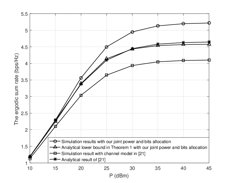
Fig. 2: Comparisons of the simulation and analytical results of the ESR v.s. PP for our proposed scheme and those in [21].

V Numerical Results

For the numerical results, we consider the systems with two different sets of distance parameters given as 𝐃1\mathbf{D}_{1} of Fig. 1 and 𝐃2=[103512371439]\mathbf{D}_{2}=\Big[\begin{smallmatrix}10&35\\ 12&37\\ 14&39\\ \end{smallmatrix}\Big] and the different number of BBs. The other major system parameters are the same as those of Fig. 1. Specifically, the systems associated with Fig. 2 - Fig. 4 and the systems associated with Fig. 5 - Fig. 6 are with 𝐃1\mathbf{D}_{1} and 𝐃2=[103512371439]\mathbf{D}_{2}=\Big[\begin{smallmatrix}10&35\\ 12&37\\ 14&39\\ \end{smallmatrix}\Big] respectively. The path-loss exponent α=4\alpha=4. Moreover, if the total transmit power PP can not support a given number of clusters (i.e., N=3N=3 at the beginning of system design), we will follow the way of (a) in the design as we have described after Remark 6. The ESR curves corresponding to the obtained analytical lower bound in Theorem 1 will be notified specifically. Otherwise, the ESR curves are obtained from simulations.

Fig. 2 shows the simulation results of the ESR v.s PP for our proposed joint bits and power allocation method and the corresponding analytical lower bound given by Theorem 1 with B=42B=42 bits. For comparisons, we also plot the simulation and analytical results with the quantized CSI model in [21]. We can see from the figure, the simulation results illustrate the fact we have explained in Remark 3, i.e., the channel model for limited feedback used in [21] actually underestimates the performance of the system with the well recognized practical channel model used in many previous works [23, 19, 20]. However, we can see in the figure that the analytical ergodic rate result derived in [21] is right over the corresponding results of the simulations. This illustrates the analysis method in [21] to ignore the statistical dependence between the useful signal and MU interference signals received at each user results in overestimation of the actual performance. The big gap between analytical and simulated results demonstrates the impact of the aforementioned dependent relationships can not be ignored in the analysis and design of the practical systems. Moreover, as transmit power varies, our obtained analytical lower bound can track the real values well.

Fig. 3 compares the ESR as a function of PP achieved by our proposed bits allocation method with those of the equal bits allocation and the bits allocation method proposed in [21] for the systems with different BBs. All schemes employ the quantized channel model in this paper and the equal power allocation among all users. We can see our bits allocation method performs the best of all. And the performance gaps between our method and the other two both increase when BB becomes large, which illustrates the advantage of our method.

Refer to caption
Fig. 3: Comparisons of the ESR v.s PP for different feedback bits allocation methods.
Refer to caption
Fig. 4: Comparisons of the number of feedback bits allocated to each user for different bits allocation methods.

Fig. 4 shows the number of feedback bits allocated to each user obtained from our method and that obtained from the method in [21] with the total feedback channel bandwidth of B=60B=60 bits. We can see that, as PP increases our method allocates more bits to the nearest users (to the BS) in each cluster, and allocates less bits to the farther users. In very high power region, our method does not allocate feedback bits for the farther user in each cluster. It is not difficult to check the results show in this figure are consistent with our analysis in Subsection IV-C. The results also can be explained by the qualitative analysis as follows. On the one hand, increasing the quantization accuracy can enhance the strength of each user’s transmit signal, and the increasing of the near users’s signal strength is more effective in enhancing the transmission rate than increasing the farther users’ signal strength. On the other hand, the system is interference-limited in high power region. Increasing the quantization accuracy of user (n,k)(n,k)’s CSI can reduce the inter-cluster interference to all users (m,k)(m,k) ∀m≠n\forall m\neq n and ∀k\forall k, but only reduces the intra-cluster interference to users (n,j)(n,j) for j>kj>k due to SIC. Thus, with equal power allocation within each cluster, increasing the quantization accuracy of user (n,k)(n,k)’s CSI is more effective in reducing the MU interference than increasing the quantization accuracy of user (n,j)(n,j)’s CSI for j>kj>k. In contrast, the bits allocation by the method of [21] does not change with the increase of PP.

Fig. 5 shows the ESR as a function of PP for different total bandwidths of feedback channels achieved respectively by our proposed joint optimization method, our bits allocation method with equal power allocation among all users, and the equal power and bits allocation method. As can be seen from the figure, our proposed power allocation converges to the equal power allocation as PP goes large, which is consistent with our analysis in Corollary 1. However, there is always a gap between the performance of equal power and bits allocation and those of the other two.

Fig. 6 compares the ESR as a function of BB achieved by our joint optimization method, our bits allocation method with equal power allocation and equal power and bits allocation method. As the baseline, we also plot the performance of the OMA transmission, where, for fair comparisons, the groups of the nearer users and the farther users share a fraction of 1/21/2 time resource using linear ZFBF with equal power allocation for transmission. As can be seen from the figure, the performance of our joint bits and power allocation method is the best of all. The performances of all NOMA transmission schemes are better than that of OMA scheme for the system setting considered. Moreover, we can observe that, the performance gap between our joint optimization scheme and the equal bits allocation scheme and also the performance gap between our joint optimization scheme and the OMA scheme both increase as the accuracy of channel quantization (BB) increases. However, the advantage of our power allocation method over the equal power allocation method decreases as the accuracy of channel quantization increases.

Refer to caption
Fig. 5: Comparison of the system ESRs as a function of PP with different power allocation methods.
Refer to caption
Fig. 6: Comparisons of the ESRs as a function of BB achieved by different power and feedback bits allocation methods.

VI Conclusions

In this paper, we have investigated the transmit-receive design, performance analysis, and optimization of downlink multi-antenna NOMA cellular networks with general limited feedback in FDD mode. A mathematically strict performance analysis of the ergodic rate for the considered system was conducted for the first time. A closed-form lower bound on the ergodic rate of each user was obtained in terms of transmit power, CSI quantization accuracy and channel conditions. Then, we optimized the two key parameters of the considered system, i.e., transmit power and the number of feedback bits allocated to each users. Finally, we conducted asymptotic performance analysis on the optimization results, and obtained insights on system design guidelines.

-A Proof of Theorem 1

According to [23, Lemma 2], we have |𝐞~n,k​𝐰i|2∼Beta​(1,M−2)\left|\tilde{\mathbf{e}}_{n,k}\mathbf{w}_{i}\right|^{2}\sim\text{Beta}(1,M-2) and 𝔼⁡[|𝐞~n,k​𝐰i|2]=(M−1)−1\mathbb{E}\left[|\tilde{\mathbf{e}}_{n,k}\mathbf{w}_{i}|^{2}\right]=(M-1)^{-1}. Then, by employing Jensen’s inequality we can lower-bound Rn,kR_{n,k} for k≥2k\geq 2 as (29) at the top of next page,

Rn,k\displaystyle R_{n,k} ≥\displaystyle\geq 𝔼⁡[log2⁡(1+dn,k−ασn,k2​|𝐡n,k​𝐰n|2​Pn,k1+Sn,k(2)​|𝐡n,k​𝐰n|2+Sn,k(3)​𝔼​[|𝐞~n,k​𝐰i|2]​‖𝐡n,k‖2​sin2⁡θn,k)]\displaystyle\mathbb{E}\left[\log_{2}\left(1+\frac{\frac{d_{n,k}^{-\alpha}}{\sigma_{n,k}^{2}}|\mathbf{h}_{n,k}\mathbf{w}_{n}|^{2}P_{n,k}}{1+S_{n,k}^{(2)}\left|\mathbf{h}_{n,k}\mathbf{w}_{n}\right|^{2}+S_{n,k}^{(3)}\mathbb{E}\left[\left|\tilde{\mathbf{e}}_{n,k}\mathbf{w}_{i}\right|^{2}\right]||\mathbf{h}_{n,k}||^{2}\sin^{2}\theta_{n,k}}\right)\right] (27)
=\displaystyle= 𝔼⁡[log2⁡(1+Sn,k(1)​|𝐡n,k​𝐰n|2+Sn,k(3)​(M−1)−1​‖𝐡n,k‖2​sin2⁡θn,k1+Sn,k(2)​|𝐡n,k​𝐰n|2+Sn,k(3)​(M−1)−1​‖𝐡n,k‖2​sin2⁡θn,k)]\displaystyle\mathbb{E}\left[\log_{2}\left(\frac{1+S_{n,k}^{(1)}\left|\mathbf{h}_{n,k}\mathbf{w}_{n}\right|^{2}+S_{n,k}^{(3)}(M-1)^{-1}||\mathbf{h}_{n,k}||^{2}\sin^{2}\theta_{n,k}}{1+S_{n,k}^{(2)}\left|\mathbf{h}_{n,k}\mathbf{w}_{n}\right|^{2}+S_{n,k}^{(3)}(M-1)^{-1}||\mathbf{h}_{n,k}||^{2}\sin^{2}\theta_{n,k}}\right)\right] (28)
=\displaystyle= 𝔼⁡[log2⁡(1+Sn,k(1)​Z​‖𝐡n,k‖2+Sn,k(3)​(M−1)−1​‖𝐡n,k‖2​sin2⁡θn,k)]\displaystyle\mathbb{E}\left[\log_{2}\left(1+S_{n,k}^{(1)}Z||\mathbf{h}_{n,k}||^{2}+S_{n,k}^{(3)}(M-1)^{-1}||\mathbf{h}_{n,k}||^{2}\sin^{2}\theta_{n,k}\right)\right]
−𝔼⁡[log2⁡(1+Sn,k(2)​Z​‖𝐡n,k‖2+Sn,k(3)​(M−1)−1​‖𝐡n,k‖2​sin2⁡θn,k)]≜Rn,kL​B​1,\displaystyle-\mathbb{E}\left[\log_{2}\left(1+S_{n,k}^{(2)}Z||\mathbf{h}_{n,k}||^{2}+S_{n,k}^{(3)}(M-1)^{-1}||\mathbf{h}_{n,k}||^{2}\sin^{2}\theta_{n,k}\right)\right]\triangleq R_{n,k}^{LB1},~~ (29)


where Z≜|𝐡~n,k​𝐰n|2∼Beta​(1,M−1)Z\triangleq|\tilde{\mathbf{h}}_{n,k}\mathbf{w}_{n}|^{2}\sim\text{Beta}(1,M-1) [23]. It has been shown in [24, Lemma 2] that, with cell approximation of vector quantization the joint distribution of the random variable (RV) pair (‖𝐡n,k‖2​sin2⁡θn,k,‖𝐡n,k‖2​cos2⁡θn,k)(||\mathbf{h}_{n,k}||^{2}\sin^{2}\theta_{n,k},||\mathbf{h}_{n,k}||^{2}\cos^{2}\theta_{n,k}) is the same as that of (I,S)(I,S), where I=δn,k​YI=\delta_{n,k}Y and S=X+(1−δn,k)​YS=X+(1-\delta_{n,k})Y with X∼Gamma​(1,1)X\sim\text{Gamma}(1,1) and Y∼Gamma​(M−1,1)Y\sim\text{Gamma}(M-1,1) being two independent RVs. Since XX, YY and ZZ are independent of each other[23], Rn,kL​B​1R_{n,k}^{LB1} in (29) can be obtained as

Rn,kL​B​1=𝔼{log2[1+Sn,k(1)Z(X+(1−δn,kY))\displaystyle R_{n,k}^{LB1}=\mathbb{E}\Big\{\log_{2}\Big[1+S_{n,k}^{(1)}Z(X+(1-\delta_{n,k}Y))
+(Sn,k(1)Z+Sn,k(3)(M−1)−1)δn,kY]}\displaystyle\hskip 85.35826pt+\Big(S_{n,k}^{(1)}Z+S_{n,k}^{(3)}(M-1)^{-1}\Big)\delta_{n,k}Y\Big]\Big\}
−𝔼{log2[1+Sn,k(2)Z(X+(1−δn,kY))\displaystyle\hskip 36.98857pt-\mathbb{E}\Big\{\log_{2}\Big[1+S_{n,k}^{(2)}Z(X+(1-\delta_{n,k}Y))
+(Sn,k(1)Z+Sn,k(3)(M−1)−1)δn,kY]}\displaystyle\hskip 85.35826pt+\Big(S_{n,k}^{(1)}Z+S_{n,k}^{(3)}(M-1)^{-1}\Big)\delta_{n,k}Y\Big]\Big\}
=𝔼Z​[Υn,k​(Sn,k(1)​Z,Sn,k(1)​Z+Sn,k(3)​(M−1)−1​δn,k)]\displaystyle=\mathbb{E}_{Z}\left[\Upsilon_{n,k}\left(S_{n,k}^{(1)}Z,~S_{n,k}^{(1)}Z+S_{n,k}^{(3)}(M-1)^{-1}\delta_{n,k}\right)\right]
−𝔼Z​[Υn,k​(Sn,k(2)​Z,Sn,k(2)​Z+Sn,k(3)​(M−1)−1​δn,k)],\displaystyle\hskip 5.69054pt-\mathbb{E}_{Z}\left[\Upsilon_{n,k}\left(S_{n,k}^{(2)}Z,~S_{n,k}^{(2)}Z+S_{n,k}^{(3)}(M-1)^{-1}\delta_{n,k}\right)\right]\hskip-2.84526pt, (30)

where Υn,k​(μ,ν)≜𝔼X,Y​[log2⁡(1+μ​X+ν​Y)]\Upsilon_{n,k}(\mu,\nu)\triangleq\mathbb{E}_{X,Y}\left[\log_{2}\left(1+\mu X+\nu Y\right)\right]. The result of 𝔼Z​[Υn,k​(a​Z,a​Z+b)]≜Θn,k​(a,b)\mathbb{E}_{Z}\left[\Upsilon_{n,k}(aZ,aZ+b)\right]\triangleq\Theta_{n,k}(a,b) is derived in Appendix -B, where Θn,k​(a,b)\Theta_{n,k}(a,b) is given in (8). Then, the result of Rn,kL​B​1R_{n,k}^{LB1} in (1) follows.

When k=1k=1, Sn,k(2)=0S_{n,k}^{(2)}=0. By replacing Sn,k(2)S_{n,k}^{(2)} in (30) with 0, we can similarly obtain

Rn,1L​B​1\displaystyle R_{n,1}^{LB1} =\displaystyle= 𝔼{log2[1+αn,1Pn,1ZX\displaystyle\mathbb{E}\Big\{\log_{2}\Big[1+\alpha_{n,1}P_{n,1}ZX (31)
+(αn,1Pn,1Z+Sn,1(3)(M−1)−1δn,1)Y]}\displaystyle\hskip 8.53581pt+\left(\alpha_{n,1}P_{n,1}Z+S_{n,1}^{(3)}(M-1)^{-1}\delta_{n,1}\right)Y\Big]\Big\}
−𝔼⁡{log2⁡[1+Sn,1(3)​(M−1)−1​δn,1​Y]}\displaystyle-\mathbb{E}\left\{\log_{2}\left[1+S_{n,1}^{(3)}(M-1)^{-1}\delta_{n,1}Y\right]\right\}
=\displaystyle= Θn,k​(αn,1​Pn,1,Sn,1(3)​(M−1)−1​δn,1)\displaystyle\Theta_{n,k}(\alpha_{n,1}P_{n,1},S_{n,1}^{(3)}(M-1)^{-1}\delta_{n,1})
−𝔼⁡[log2⁡(1+Sn,1(3)​(M−1)−1​δn,1​Y)].\displaystyle-\mathbb{E}\left[\log_{2}\left(1+S_{n,1}^{(3)}(M-1)^{-1}\delta_{n,1}Y\right)\right].~~~

The second term in (31) can be obtained as

𝔼⁡[log2⁡(1+Sn,1(3)​(M−1)−1​δn,1​Y)]\displaystyle\mathbb{E}\left[\log_{2}\left(1+S_{n,1}^{(3)}(M-1)^{-1}\delta_{n,1}Y\right)\right]
=∫0+∞log2⁡(1+Sn,1(3)​(M−1)−1​δn,1​y)​e−y​yM−2(M−2)!​𝑑y\displaystyle=\int_{0}^{+\infty}\log_{2}\left(1+S_{n,1}^{(3)}(M-1)^{-1}\delta_{n,1}y\right)\frac{e^{-y}y^{M-2}}{(M-2)!}~dy
=log2⁡(e)​exp⁡(M−1Sn,1(3)​δn,1)​∑q=1M−1Eq​(M−1Sn,1(3)​δn,1),\displaystyle=\log_{2}(e)\exp\left(\frac{M-1}{S_{n,1}^{(3)}\delta_{n,1}}\right)\sum_{q=1}^{M-1}E_{q}\left(\frac{M-1}{S_{n,1}^{(3)}\delta_{n,1}}\right), (32)

where (-A) follows by using (-B) in Appendix -B. Then, Rn,kL​B​1R_{n,k}^{LB1} in (1) for k=1k=1 follows by substituting (-A) into (31).

-B The derivation of 𝔼Z​[Υn,k​(a​Z,a​Z+b)]≜Θn,k​(a,b)\mathbb{E}_{Z}\left[\Upsilon_{n,k}(aZ,aZ+b)\right]\triangleq\Theta_{n,k}(a,b) for a>0a>0, b>0b>0

Using the result in [29], the probability density function (PDF) of Jμ,ν=μ​X+ν​YJ_{\mu,\nu}=\mu X+\nu Y for μ≠ν\mu\neq\nu is given by fJμ,ν​(x)=(−1)M−1​μM−2(ν−μ)M−1​e−xμ+∑p=1M−1(−μ)p−1(M−1−p)!​(ν−μ)p​νM−1−p​xM−1−p​e−xν​(x>0)f_{J_{\mu,\nu}}(x)=\frac{(-1)^{M-1}\mu^{M-2}}{(\nu-\mu)^{M-1}}e^{-\frac{x}{\mu}}+\sum_{p=1}^{M-1}\frac{(-\mu)^{p-1}}{(M-1-p)!(\nu-\mu)^{p}\nu^{M-1-p}}x^{M-1-p}e^{-\frac{x}{\nu}}~{(x>0)}. Thus,

Υn,k​(μ,ν)=𝔼X,Y​[log2⁡(1+μ​X+ν​Y)]\displaystyle\Upsilon_{n,k}(\mu,\nu)=\mathbb{E}_{X,Y}\left[\log_{2}\left(1+\mu X+\nu Y\right)\right]
=∫0+∞log2⁡(1+x)​fJμ,ν​(x)​𝑑x\displaystyle=\int_{0}^{+\infty}\log_{2}(1+x)f_{J_{\mu,\nu}}(x)~dx
=log2(e)[(−μ)M−1(ν−μ)M−1exp(1μ)E1(1μ)\displaystyle=\log_{2}(e)\Bigg[\frac{(-\mu)^{M-1}}{(\nu-\mu)^{M-1}}\exp\left(\frac{1}{\mu}\right)E_{1}\left(\frac{1}{\mu}\right)
+∑p=1M−1(−μ)p−1​ν(ν−μ)pexp(1ν)∑q=1M−pEq(1ν)],\displaystyle\hskip 11.38109pt+\sum_{p=1}^{M-1}\frac{(-\mu)^{p-1}\nu}{(\nu-\mu)^{p}}\exp\left(\frac{1}{\nu}\right)\sum_{q=1}^{M-p}E_{q}\left(\frac{1}{\nu}\right)\Bigg],~~~~~~ (33)

where (-B) follows from the result of [30, (78)]

∫0+∞ln⁡(1+a​x)​e−μ​x​xp−1​𝑑x\displaystyle\int_{0}^{+\infty}\ln(1+ax)e^{-\mu x}x^{p-1}dx
=(p−1)!​eμa​μ−p​∑q=1pEq​(μa).\displaystyle=(p-1)!e^{\frac{\mu}{a}}\mu^{-p}\sum_{q=1}^{p}E_{q}\left(\frac{\mu}{a}\right). (34)

Then, substituting μ=a​Z\mu=aZ and ν=a​Z+b\nu=aZ+b with a,b>0a,b>0 in to (-B), we can obtain

𝔼Z​[Υn,k​(a​Z,a​Z+b)]\displaystyle\mathbb{E}_{Z}\left[\Upsilon_{n,k}(aZ,aZ+b)\right]
=log2(e)𝔼Z[(−a​Z)M−1bM−1exp(1a​Z)E1(1a​Z)\displaystyle=\log_{2}(e)\mathbb{E}_{Z}\Bigg[\frac{(-aZ)^{M-1}}{b^{M-1}}\exp\bigg(\frac{1}{aZ}\bigg)E_{1}\bigg(\frac{1}{aZ}\bigg)
+∑p=1M−1(−a​Z)p−1​(a​Z+b)bpexp(1a​Z+b)\displaystyle\hskip 62.59605pt+\sum_{p=1}^{M-1}\frac{(-aZ)^{p-1}(aZ+b)}{b^{p}}\exp\bigg(\frac{1}{aZ+b}\bigg)
×∑q=1M−pEq(1a​Z+b)].\displaystyle\hskip 62.59605pt\times\sum_{q=1}^{M-p}E_{q}\bigg(\frac{1}{aZ+b}\bigg)\Bigg]. (35)

By using the relationship[27] Eq​(x)=1q−1​[e−x−x​Eq−1​(x)]E_{q}(x)=\frac{1}{q-1}\left[e^{-x}-xE_{q-1}(x)\right] and E1​(x)=−Ei​(−x)E_{1}(x)=-E_{i}(-x) with induction, Eq​(x)E_{q}(x) can be expressed with Ei​(−x)E_{i}(-x) as Eq​(x)=e−x​∑s=0q−2(q−s−2)!​(−x)s(q−1)!+(−1)q​(x)q−1(q−1)!​Ei​(−x)E_{q}(x)=e^{-x}\sum_{s=0}^{q-2}\frac{(q-s-2)!(-x)^{s}}{(q-1)!}+\frac{(-1)^{q}(x)^{q-1}}{(q-1)!}E_{i}(-x). Then, substituting this result into (-B) with the PDF of ZZ, we can obtain

𝔼Z​[Υn,k​(a​Z,a​Z+b)]\displaystyle\mathbb{E}_{Z}\left[\Upsilon_{n,k}(aZ,aZ+b)\right] (36)
=\displaystyle= log2(e)𝔼Z[(−1)M​(a​Z)M−1bM−1exp(1a​Z)Ei(−1a​Z)\displaystyle\log_{2}(e)\mathbb{E}_{Z}\Bigg[\frac{(-1)^{M}(aZ)^{M-1}}{b^{M-1}}\exp\left(\frac{1}{aZ}\right)E_{i}\left(-\frac{1}{aZ}\right)
+∑p=1M−1∑q=1M−p(−1)p+q+1​(a​Z)p−1(q−1)!​bp​(a​Z+b)q−2\displaystyle+\sum_{p=1}^{M-1}\sum_{q=1}^{M-p}\frac{(-1)^{p+q+1}(aZ)^{p-1}}{(q-1)!b^{p}(aZ+b)^{q-2}}
×exp⁡(1a​Z+b)​Ei​(−1a​Z+b)\displaystyle\hskip 56.9055pt\times\exp\left(\frac{1}{aZ+b}\right)E_{i}\left(-\frac{1}{aZ+b}\right)
+∑p=1M−1∑q=2M−p∑s=0q−2(−1)p+s−1​(q−s−2)!​(a​Z)p−1(q−1)!​bp​(a​Z+b)s−1],\displaystyle+\sum_{p=1}^{M-1}\sum_{q=2}^{M-p}\sum_{s=0}^{q-2}\frac{(-1)^{p+s-1}(q-s-2)!(aZ)^{p-1}}{(q-1)!b^{p}(aZ+b)^{s-1}}\Bigg],

which is given by (8) with

I1​(a)≜∫01(a​z)M−1​(1−z)M−2​exp⁡(1a​z)​Ei​(−1a​z)​𝑑z,\displaystyle I_{1}(a)\triangleq\int_{0}^{1}(az)^{M-1}(1-z)^{M-2}\exp\bigg(\frac{1}{az}\bigg)E_{i}\bigg(\hskip-4.2679pt-\frac{1}{az}\bigg)dz,
(37)
I2​(a,b,p,q)≜∫01(a​z)p−1​(1−z)M−2(a​z+b)q−2​exp⁡(1a​z+b)\displaystyle I_{2}(a,b,p,q)\triangleq\int_{0}^{1}\frac{(az)^{p-1}(1-z)^{M-2}}{(az+b)^{q-2}}\exp\left(\frac{1}{az+b}\right)
×Ei​(−1a​z+b)​d​z,\displaystyle\hskip 113.81102pt\times E_{i}\left(-\frac{1}{az+b}\right)dz, (38)
I3​(a,b,p,s)≜∫01(a​z)p−1​(1−z)M−2(a​z+b)s−1​𝑑z.\displaystyle I_{3}(a,b,p,s)\triangleq\int_{0}^{1}\frac{(az)^{p-1}(1-z)^{M-2}}{(az+b)^{s-1}}dz. (39)

Then, we derive the results of (37), (-B) and (39) as follows. For the convenience of presentation, we first define an integral Ψ⁡(n,u,v)=∫uvxn​ex​Ei​(−x)​𝑑x\Psi(n,u,v)=\int_{u}^{v}x^{n}e^{x}E_{i}(-x)dx, whose closed-form result is given by (1) for different cases. The derivation is provided in Appendix -C. Then, I1​(a)I_{1}(a) can be obtained as

I1​(a)=∑t=0M−2(M−2t)​(−1)tat​∫01(a​z)M−1+t\displaystyle I_{1}(a)=\sum_{t=0}^{M-2}{M-2\choose t}\frac{(-1)^{t}}{a^{t}}\int_{0}^{1}(az)^{M-1+t}
×exp⁡(1a​z)​Ei​(−1a​z)​d​z\displaystyle\hskip 113.81102pt\times\exp\left(\frac{1}{az}\right)E_{i}\left(-\frac{1}{az}\right)dz
=∑t=0M−2(M−2t)​(−1)tat​∫+∞1ax−M+1−t​ex​Ei​(−x)​d​(1a​x)\displaystyle=\sum_{t=0}^{M-2}{M-2\choose t}\frac{(-1)^{t}}{a^{t}}\int_{+\infty}^{\frac{1}{a}}x^{-M+1-t}e^{x}E_{i}(-x)~d\left(\frac{1}{ax}\right)
(40)
=∑t=0M−2(M−2t)​(−1)tat+1​Ψ​(−M−1−t,1a,v)|v→+∞,\displaystyle=\sum_{t=0}^{M-2}{M-2\choose t}\frac{(-1)^{t}}{a^{t+1}}\Psi\left(-M-1-t,\frac{1}{a},v\right)\bigg|_{v\to+\infty},

where (40) follows by the change of variables x=1a​zx=\frac{1}{az}. Similarly, I2​(a,b,p,q)I_{2}(a,b,p,q) can be obtained by using the change of variables x=1a​z+bx=\frac{1}{az+b} as

I2​(a,b,p,q)=∫1b1a+b(1x−b)p−1​[1−1a​(1x−b)]M−2\displaystyle I_{2}(a,b,p,q)=\int_{\frac{1}{b}}^{\frac{1}{a+b}}\left(\frac{1}{x}-b\right)^{p-1}\left[1-\frac{1}{a}\left(\frac{1}{x}-b\right)\right]^{M-2}
×xq−2​ex​Ei​(−x)​d​[1a​(1x−b)]\displaystyle\hskip 85.35826pt\times x^{q-2}e^{x}E_{i}(-x)~d\left[\frac{1}{a}\left(\frac{1}{x}-b\right)\right]
=∑r=0M−2∑t=0p−1+r(M−2r)​(p−1+rt)​(−1)p−1−t​bp−1+r−tar+1\displaystyle=\sum_{r=0}^{M-2}\sum_{t=0}^{p-1+r}{M-2\choose r}{p-1+r\choose t}\frac{(-1)^{p-1-t}b^{p-1+r-t}}{a^{r+1}}
×∫1a+b1bxq−4−t​ex​Ei​(−x)​𝑑x\displaystyle\hskip 113.81102pt\times\int_{\frac{1}{a+b}}^{\frac{1}{b}}x^{q-4-t}e^{x}E_{i}(-x)~dx
=∑r=0M−2∑t=0p−1+r(M−2r)​(p−1+rt)​(−1)p−1−t​bp−1+r−tar+1\displaystyle=\sum_{r=0}^{M-2}\sum_{t=0}^{p-1+r}{M-2\choose r}{p-1+r\choose t}\frac{(-1)^{p-1-t}b^{p-1+r-t}}{a^{r+1}}
×Ψ⁡(q−4−t,1a+b,1b).\displaystyle\hskip 113.81102pt\times\Psi\left(q-4-t,\frac{1}{a+b},\frac{1}{b}\right).

Finally, I3​(a,b,p,s)I_{3}(a,b,p,s) can be obtained as

I3​(a,b,p,s)\displaystyle I_{3}(a,b,p,s)
=∑t=0M−2(M−2t)​(−a)−t​∫01(a​z)p−1+t(a​z+b)s−1​𝑑z\displaystyle=\sum_{t=0}^{M-2}{M-2\choose t}(-a)^{-t}\int_{0}^{1}\frac{(az)^{p-1+t}}{(az+b)^{s-1}}dz
=∑t=0M−2(M−2t)​(−1)t​a−t−1​∫0axp−1+t(x+b)s−1​𝑑x\displaystyle=\sum_{t=0}^{M-2}{M-2\choose t}(-1)^{t}a^{-t-1}\int_{0}^{a}\frac{x^{p-1+t}}{(x+b)^{s-1}}dx
=∑t=0M−2(M−2t)​(−1)t​a−t−1bs−1​∫0axp−1+t(xb+1)s−1​𝑑x\displaystyle=\sum_{t=0}^{M-2}{M-2\choose t}\frac{(-1)^{t}a^{-t-1}}{b^{s-1}}\int_{0}^{a}\frac{x^{p-1+t}}{(\frac{x}{b}+1)^{s-1}}dx (41)
=∑t=0M−2(M−2t)​(−1)t​a−t−1bs−1⋅ap+t(p+t)\displaystyle=\sum_{t=0}^{M-2}{M-2\choose t}\frac{(-1)^{t}a^{-t-1}}{b^{s-1}}\cdot\frac{a^{p+t}}{(p+t)}
×F12​(s−1,p+t,p+t+1,−ab)\displaystyle\hskip 56.9055pt\times~{{}_{2}}F_{1}\left(s-1,p+t;p+t+1;-\frac{a}{b}\right)~~~~ (42)
=∑t=0M−2(M−2t)​(−1)t​ap−1bs−1​(p+t)\displaystyle=\sum_{t=0}^{M-2}{M-2\choose t}\frac{(-1)^{t}a^{p-1}}{b^{s-1}(p+t)}
×F12​(s−1,p+t,p+t+1,−ab),\displaystyle\hskip 56.9055pt\times~{{}_{2}}F_{1}\left(s-1,p+t;p+t+1;-\frac{a}{b}\right),

where (41) is obtained from the change of variables x=a​zx=az and (-B) follows from [27, 3.194.1] ∫0uxμ−1​d​x(1+β​x)ν=uμμ​F12​(ν,μ,1+μ,−β​u)\int_{0}^{u}\frac{x^{\mu-1}dx}{(1+\beta x)^{\nu}}=\frac{u^{\mu}}{\mu}{{}_{2}}F_{1}(\nu,\mu;1+\mu;-\beta u). Then, the final results can be obtained by substituting the results of I1​(a)I_{1}(a), I2​(a,b,p,q)I_{2}(a,b,p,q) and I3​(a,b,p,s)I_{3}(a,b,p,s) into (36).

-C Derivation of Ψ⁡(n,u,v)\Psi(n,u,v)

First, for n>0n>0, Ψ⁡(n,u,v)\Psi(n,u,v) can be obtained by integration by parts as

Ψ⁡(n,u,v)\displaystyle\hskip-14.22636pt\Psi(n,u,v) =\displaystyle= ∫uvEi​(−x)​d​[ex​∑k=0n(−1)k​n!(n−k)!​xn−k]\displaystyle\int_{u}^{v}E_{i}(-x)~d\left[e^{x}\sum_{k=0}^{n}\frac{(-1)^{k}n!}{(n-k)!}x^{n-k}\right] (44)
=\displaystyle= [Ei​(−x)​ex​∑k=0n(−1)k​n!(n−k)!​xn−k]uv\displaystyle\left[E_{i}(-x)e^{x}\sum_{k=0}^{n}\frac{(-1)^{k}n!}{(n-k)!}x^{n-k}\right]_{u}^{v}
−∫uvex∑k=0n(−1)k​n!(n−k)!xn−kd[Ei(−x)]\displaystyle-\int_{u}^{v}e^{x}\sum_{k=0}^{n}\frac{(-1)^{k}n!}{(n-k)!}x^{n-k}~d[E_{i}(-x)]
=\displaystyle= [Ei​(−x)​ex​∑k=0n(−1)k​n!(n−k)!​xn−k]uv\displaystyle\left[E_{i}(-x)e^{x}\sum_{k=0}^{n}\frac{(-1)^{k}n!}{(n-k)!}x^{n-k}\right]_{u}^{v}
−∑k=0n(−1)k​n!(n−k)!∫uvxn−k−1dx,\displaystyle-\sum_{k=0}^{n}\frac{(-1)^{k}n!}{(n-k)!}\int_{u}^{v}x^{n-k-1}~dx,

which is given in (1) with n>0n>0, where (44) follows from the result [27, 2.321.2] ∫xn​ea​x​𝑑x=ea​x​(∑k=0n(−1)k​n!ak+1​(n−k)!​xn−k)\int x^{n}e^{ax}dx=e^{ax}\Big(\sum_{k=0}^{n}\frac{(-1)^{k}n!}{a^{k+1}(n-k)!}x^{n-k}\Big) and (44) follows from (Ei​(−x))′=x−1​e−x\left(E_{i}(-x)\right)^{\prime}=x^{-1}e^{-x}.

For n=0n=0, we can similarly obtain

Ψ⁡(0,u,v)=∫uvEi​(−x)​d​ex=ex​Ei​(−x)|uv−∫uvx−1​𝑑x\displaystyle\Psi(0,u,v)=\int_{u}^{v}E_{i}(-x){\rm d}e^{x}=e^{x}E_{i}(-x)\Big|_{u}^{v}-\int_{u}^{v}x^{-1}{\rm d}x
=ev​Ei​(−v)−eu​Ei​(−u)−ln⁡(vu).\displaystyle\hskip 44.10176pt=e^{v}E_{i}(-v)-e^{u}E_{i}(-u)-\ln\left(\frac{v}{u}\right).

For n≤−2n\leq-2, Ψ⁡(n,u,v)\Psi(n,u,v) can be obtained as

Ψ(n,u,v)=∫uvEi(−x)d[−ex∑k=1−n−1(−n−k−1)!(−n−1)!xn+k\displaystyle\Psi(n,u,v)=\int_{u}^{v}E_{i}(-x)d\Bigg[\hskip-2.84526pt-e^{x}\sum_{k=1}^{-n-1}\frac{(-n-k-1)!}{(-n-1)!}x^{n+k}
+Ei​(x)(−n−1)!]\displaystyle\hskip 156.49014pt+\frac{E_{i}(x)}{(-n-1)!}\Bigg] (45)
=[Ei(−x)(−ex∑k=1−n−1(−n−k−1)!(−n−1)!xn+k\displaystyle=\Bigg[E_{i}(-x)\Bigg(-e^{x}\sum_{k=1}^{-n-1}\frac{(-n-k-1)!}{(-n-1)!}x^{n+k}
+Ei​(x)(−n−1)!)]uv\displaystyle\hskip 156.49014pt+\frac{E_{i}(x)}{(-n-1)!}\Bigg)\Bigg]_{u}^{v}
−∫uv(−ex∑k=1−n−1(−n−k−1)!(−n−1)!xn+k\displaystyle-\int_{u}^{v}\Bigg(-e^{x}\sum_{k=1}^{-n-1}\frac{(-n-k-1)!}{(-n-1)!}x^{n+k}
OPEN+Ei​(x)(−n−1)!)​d​[Ei​(−x)],\displaystyle\hskip 113.81102pt+\frac{E_{i}(x)}{(-n-1)!}\Bigg)~d[E_{i}(-x)], (46)

where (-C) follows from the result [27, 2.324.2] ∫ea​xxndx=−ea​x∑k=1n−1(n−k−1)!​ak−1(n−1)!​xn−k+an−1​Ei​(a​x)(n−1)!(n>0)\int\frac{e^{ax}}{x^{n}}dx=-e^{ax}\sum_{k=1}^{n-1}\frac{(n-k-1)!a^{k-1}}{(n-1)!x^{n-k}}+\frac{a^{n-1}E_{i}(ax)}{(n-1)!}(n>0) with a=1a=1. Moreover, ∫uvEi​(x)​d​[Ei​(−x)]\int_{u}^{v}E_{i}(x)~d[E_{i}(-x)] can be obtained as

∫uvEi​(x)​d​[Ei​(−x)]=∫uv(Ei​(−x)CLOSE\displaystyle\int_{u}^{v}E_{i}(x)~d[E_{i}(-x)]=\int_{u}^{v}\bigg(E_{i}(-x)
+∑m=0∞2​x2​m+1(2​m+1)​(2​m+1)!)d[Ei(−x)]\displaystyle\hskip 42.67912pt+\sum_{m=0}^{\infty}\frac{2x^{2m+1}}{(2m+1)(2m+1)!}\bigg)~d[E_{i}(-x)] (47)
=12​Ei2​(−x)|uv+∑m=0∞2(2​m+1)​(2​m+1)!\displaystyle=\frac{1}{2}E_{i}^{2}(-x)\Big|_{u}^{v}+\sum_{m=0}^{\infty}\frac{2}{(2m+1)(2m+1)!}
×(∫0vx2​m​e−x​𝑑x−∫0ux2​m​e−x​𝑑x)\displaystyle\hskip 42.67912pt\times\left(\int_{0}^{v}x^{2m}e^{-x}~dx-\int_{0}^{u}x^{2m}e^{-x}~dx\right)
=12​[Ei2​(−v)−Ei2​(−u)]+∑m=0∞∑l=02​m2​(ul​e−u−vl​e−v)(2​m+1)2​l!,\displaystyle=\frac{1}{2}\left[E_{i}^{2}(-v)-E_{i}^{2}(-u)\right]+\sum_{m=0}^{\infty}\sum_{l=0}^{2m}\frac{2(u^{l}e^{-u}-v^{l}e^{-v})}{(2m+1)^{2}\,l!},

where (-C) follows from[27, 8.214.3] Ei​(x)=Ei​(−x)+∑m=0∞2​x2​m+1(2​m+1)​(2​m+1)!E_{i}(x)=E_{i}(-x)+\sum_{m=0}^{\infty}\frac{2x^{2m+1}}{(2m+1)(2m+1)!} and (-C) follows from [27, 3.351.1]. Then, the expression of Ψ⁡(n,u,v)\Psi(n,u,v) for n≤−2n\leq-2 in (1) can be obtained by combing (-C) and (-C). Similarly, for n=−1n=-1, we can obtain

Ψ⁡(−1,u,v)=∫uvx−1​ex​Ei​(−x)​𝑑x=∫uvEi​(−x)​d​Ei​(x)\displaystyle\Psi(-1,u,v)=\int_{u}^{v}x^{-1}e^{x}E_{i}(-x)~dx=\int_{u}^{v}E_{i}(-x)~dE_{i}(x)
=[Ei​(−x)​Ei​(x)]uv−∫uvEi​(x)​d​[Ei​(−x)],\displaystyle\hskip 51.21504pt=\left[E_{i}(-x)E_{i}(x)\right]_{u}^{v}-\hskip-2.84526pt\int_{u}^{v}E_{i}(x)~d[E_{i}(-x)], (49)

which is given by (1) with n=−1n=-1. Here, we employ again [27, 3.351.1].

For n<−1n<-1 with v→+∞v\to+\infty, we can obtain

Ψ~​(n,u)=Ψ⁡(n,u,v)|v→+∞=∫u∞xn​ex​Ei​(−x)​𝑑x\displaystyle\tilde{\Psi}(n,u)=\Psi(n,u,v)\big|_{v\to+\infty}=\int_{u}^{\infty}x^{n}e^{x}E_{i}(-x)~dx
=[Ei(−x)(−ex∑k=1−n−1(−n−k−1)!(−n−1)!xn+k\displaystyle=\Bigg[E_{i}(-x)\Bigg(-e^{x}\sum_{k=1}^{-n-1}\frac{(-n-k-1)!}{(-n-1)!}x^{n+k}
+Ei​(x)(−n−1)!)]u∞+[∑k=1−n−1(−n−k−1)!​xn+k(−n−1)!​(n+k)]u∞\displaystyle\hskip 11.38109pt+\frac{E_{i}(x)}{(-n-1)!}\Bigg)\Bigg]_{u}^{\infty}+\left[\sum_{k=1}^{-n-1}\frac{(-n-k-1)!~x^{n+k}}{(-n-1)!(n+k)}\right]_{u}^{\infty}
−1(−n−1)!∫u∞Ei(x)d[Ei(−x)].\displaystyle\hskip 11.38109pt-\frac{1}{(-n-1)!}\int_{u}^{\infty}E_{i}(x)~d[E_{i}(-x)]. (50)

According to [31, 5.1.19], we have 1x+1<ex​E1​(x)≤1x​(x>0)\frac{1}{x+1}<e^{x}E_{1}(x)\leq\frac{1}{x}~(x>0). Since E1​(x)=−Ei​(−x)E_{1}(x)=-E_{i}(-x), we have −1x<ex​Ei​(−x)≤−1x+1​(x>0)-\frac{1}{x}<e^{x}E_{i}(-x)\leq-\frac{1}{x+1}~(x>0). Then, it is easy to see limx→+∞ex​Ei​(−x)=0\lim\limits_{x\to+\infty}e^{x}E_{i}(-x)=0. In addition, using L’Hospital rule it is easy to obtain limx→+∞Ei​(−x)​Ei​(x)=0\lim\limits_{x\to+\infty}E_{i}(-x)E_{i}(x)=0. Thus, for n+k<0n+k<0, the first term in (-C) can be obtained as [Ei(−x)(−ex∑k=1−n−1(−n−k−1)!(−n−1)!xn+k+Ei​(x)(−n−1)!)]u∞=Ei(−u)(eu∑k=1−n−1(−n−k−1)!(−n−1)!un+k−Ei​(u)(−n−1)!)\left[E_{i}(-x)\left(-e^{x}\sum_{k=1}^{-n-1}\frac{(-n-k-1)!}{(-n-1)!}x^{n+k}+\frac{E_{i}(x)}{(-n-1)!}\right)\right]_{u}^{\infty}=E_{i}(-u)\left(e^{u}\sum_{k=1}^{-n-1}\frac{(-n-k-1)!}{(-n-1)!}u^{n+k}-\frac{E_{i}(u)}{(-n-1)!}\right). The second term in (-C) is given by [∑k=1−n−1(−n−k−1)!​xn+k(−n−1)!​(n+k)]u∞=−∑k=1−n−1(−n−k−1)!​un+k(−n−1)!​(n+k)\bigg[\sum_{k=1}^{-n-1}\frac{(-n-k-1)!~x^{n+k}}{(-n-1)!(n+k)}\bigg]_{u}^{\infty}=-\sum_{k=1}^{-n-1}\frac{(-n-k-1)!~u^{n+k}}{(-n-1)!(n+k)}. Similar to (-C), the third term in (-C) can be obtained as ∫u+∞Ei​(x)​d​[Ei​(−x)]=−12​Ei2​(−u)+∑m=0∞∑l=02​m2​ul​e−u(2​m+1)2​l!\int_{u}^{+\infty}E_{i}(x)~d[E_{i}(-x)]=-\frac{1}{2}E_{i}^{2}(-u)+\sum_{m=0}^{\infty}\sum_{l=0}^{2m}\frac{2u^{l}e^{-u}}{(2m+1)^{2}\,l!}, where we have used [27, 3.351.2]. Then, the result of Ψ⁡(n,u,v)|v→+∞\Psi(n,u,v)\big|_{v\to+\infty} in (1) follows by substituting the above results into (-C).

-D Proof of Theorem 2

With the expressions of Rn,ki​d​e​a​lR_{n,k}^{ideal} and Rn,kR_{n,k} we have

Δ​Rn,k=𝔼⁡[log2⁡(1+Sn,k(1)​|𝐡n,k​𝐰n|2)]\displaystyle\Delta R_{n,k}=\mathbb{E}\left[\log_{2}\left(1+S_{n,k}^{(1)}\left|\mathbf{h}_{n,k}\mathbf{w}_{n}\right|^{2}\right)\right]\hskip-14.22636pt
−𝔼[log2(1+Sn,k(2)|𝐡n,k𝐰n|2)]−𝔼[log2(1+Sn,k(1)|𝐡n,k𝐰n|2\displaystyle-\mathbb{E}\left[\log_{2}\left(1+S_{n,k}^{(2)}\left|\mathbf{h}_{n,k}\mathbf{w}_{n}\right|^{2}\right)\right]\hskip-2.84526pt-\hskip-1.70717pt\mathbb{E}\Bigg[\log_{2}\bigg(1+S_{n,k}^{(1)}\left|\mathbf{h}_{n,k}\mathbf{w}_{n}\right|^{2}\hskip-14.22636pt
+dn,k−ασn,k2sin2θn,k||𝐡n,k||2∑i=1,i≠nN|𝐞~n,k𝐰i|2∑l=1KPi,l)]\displaystyle\hskip 28.45274pt+\frac{d_{n,k}^{-\alpha}}{\sigma_{n,k}^{2}}\sin^{2}\theta_{n,k}||\mathbf{h}_{n,k}||^{2}\sum_{i=1,i\neq n}^{N}\left|\tilde{\mathbf{e}}_{n,k}\mathbf{w}_{i}\right|^{2}\sum_{l=1}^{K}P_{i,l}\bigg)\Bigg]\hskip-14.22636pt
+𝔼[log2(1+Sn,k(2)|𝐡n,k𝐰n|2+dn,k−ασn,k2sin2θn,k||𝐡n,k||2\displaystyle\hskip 5.69054pt+~\mathbb{E}\Bigg[\log_{2}\Bigg(1+S_{n,k}^{(2)}\left|\mathbf{h}_{n,k}\mathbf{w}_{n}\right|^{2}+\frac{d_{n,k}^{-\alpha}}{\sigma_{n,k}^{2}}\sin^{2}\theta_{n,k}||\mathbf{h}_{n,k}||^{2}\hskip-14.22636pt
×∑i=1,i≠nN|𝐞~n,k𝐰i|2∑l=1KPi,l)]\displaystyle\hskip 71.13188pt\times\sum_{i=1,i\neq n}^{N}\left|\tilde{\mathbf{e}}_{n,k}\mathbf{w}_{i}\right|^{2}\sum_{l=1}^{K}P_{i,l}\Bigg)\Bigg]\hskip-14.22636pt (51)
≤𝔼[log2(1+Sn,k(2)|𝐡n,k𝐰n|2+dn,k−ασn,k2sin2θn,k||𝐡n,k||2\displaystyle\leq\mathbb{E}\Bigg[\log_{2}\Bigg(1+S_{n,k}^{(2)}\left|\mathbf{h}_{n,k}\mathbf{w}_{n}\right|^{2}+\frac{d_{n,k}^{-\alpha}}{\sigma_{n,k}^{2}}\sin^{2}\theta_{n,k}||\mathbf{h}_{n,k}||^{2}\hskip-14.22636pt (52)
×∑i=1,i≠nN|𝐞~n,k𝐰i|2∑l=1KPi,l)]−𝔼[log2(1+Sn,k(2)|𝐡n,k𝐰n|2])\displaystyle\hskip 2.84526pt\times\hskip-2.84526pt\sum_{i=1,i\neq n}^{N}\left|\tilde{\mathbf{e}}_{n,k}\mathbf{w}_{i}\right|^{2}\sum_{l=1}^{K}P_{i,l}\Bigg)\Bigg]\hskip-2.84526pt-\hskip-1.70717pt\mathbb{E}\left[\log_{2}\left(1+S_{n,k}^{(2)}\left|\mathbf{h}_{n,k}\mathbf{w}_{n}\right|^{2}\right]\right)\hskip-14.22636pt
≤log2⁡(1+Sn,k(2)+MM−1​2Bn,k​β​(2Bn,k,MM−1)​Sn,k(3))\displaystyle\leq\log_{2}\left(1+S_{n,k}^{(2)}+\frac{M}{M-1}2^{B_{n,k}}\beta\left(2^{B_{n,k}},\frac{M}{M-1}\right)S_{n,k}^{(3)}\right)\hskip-14.22636pt
−log2⁡(e)​e1Sn,k(2)​E1​(1Sn,k(2))\displaystyle\hskip 22.76219pt-\log_{2}(e)e^{\frac{1}{S_{n,k}^{(2)}}}E_{1}\left(\small{\frac{1}{S_{n,k}^{(2)}}}\right)\hskip-14.22636pt
=log2⁡(1+Sn,k(2)+Γ⁡(2​M−1M−1)​2−Bn,kM−1​Sn,k(3))\displaystyle=\log_{2}\left(1+S_{n,k}^{(2)}+\Gamma\left(\frac{2M-1}{M-1}\right)2^{-\frac{B_{n,k}}{M-1}}S_{n,k}^{(3)}\right)\hskip-14.22636pt
−log2⁡(e)​e1Sn,k(2)​E1​(1Sn,k(2)),\displaystyle\hskip 22.76219pt-\log_{2}(e)e^{\frac{1}{S_{n,k}^{(2)}}}E_{1}\left(\small{\frac{1}{S_{n,k}^{(2)}}}\right), (53)

where (52) follows by neglecting dn,k−ασn,k2​sin2⁡θn,k​‖𝐡n,k‖2​∑i=1,i≠nN|𝐞~n,k​𝐰i|2​∑l=1KPi,l\frac{d_{n,k}^{-\alpha}}{\sigma_{n,k}^{2}}\sin^{2}\theta_{n,k}||\mathbf{h}_{n,k}||^{2}\sum_{i=1,i\neq n}^{N}\left|\tilde{\mathbf{e}}_{n,k}\mathbf{w}_{i}\right|^{2}\sum_{l=1}^{K}P_{i,l} in the third log2\log_{2} of (51). (-D) is obtained by applying Jensen’s inequality to the first log2\log_{2} term of (52). (-D) follows by combing the results 𝔼⁡[|𝐡n,k​𝐰n|2]=1\mathbb{E}[|\mathbf{h}_{n,k}\mathbf{w}_{n}|^{2}]=1, 𝔼⁡[‖𝐡n,k‖2]=M\mathbb{E}[||\mathbf{h}_{n,k}||^{2}]=M and 𝔼⁡[sin2⁡θn,k]=2Bn,k​β​(2Bn,k,MM−1)\mathbb{E}[\sin^{2}\theta_{n,k}]=2^{B_{n,k}}\beta\Big(2^{B_{n,k}},\frac{M}{M-1}\Big) with 2Bn,k​β​(2Bn,k,MM−1)≈Γ⁡(MM−1)​2−Bn,kM−12^{B_{n,k}}\beta\left(2^{B_{n,k}},\frac{M}{M-1}\right)\approx\Gamma\left(\frac{M}{M-1}\right)2^{-\frac{B_{n,k}}{M-1}} and x​Γ​(x)=Γ⁡(x+1)x\Gamma(x)=\Gamma(x+1), which were shown in [23].

-E Proof of Theorem 3

It is easy to show that the objective function is logarithm convex function of variables Bn,kB_{n,k}s. Thus, the problem of (IV-A) is a convex optimization problem. The Lagrangian is given by

ℒ⁡(Bn,k,λ)=λ⁡(∑n=1N∑k=1KBn,k−B)\displaystyle\mathcal{L}(B_{n,k},\lambda)=\lambda\left(\sum_{n=1}^{N}\sum_{k=1}^{K}B_{n,k}-B\right)
+∏n=1N∏k=1K(1+Sn,k(2)+Γ(2​M−1M−1)2−Bn,kM−1Sn,k(3)),\displaystyle\hskip 22.76219pt+\prod_{n=1}^{N}\prod_{k=1}^{K}\left(1+S_{n,k}^{(2)}+\Gamma\left(\frac{2M-1}{M-1}\right)2^{-\frac{B_{n,k}}{M-1}}S_{n,k}^{(3)}\right),

where λ\lambda is the is the Lagrange multiplier associated with total feedback bits constraint. Applying the Karush-Kuhn-Tucker (KKT) condition, we can get the necessary and sufficient conditions as

∂ℒ∂Bn,k|Bn,k⋆,λ⋆=−ln⁡(2)​Γ​(2​M−1M−1)​Sn,k(3)​2−Bn,kM−1(M−1)\displaystyle\frac{\partial\mathcal{L}}{\partial B_{n,k}}\Bigg|_{B^{\star}_{n,k},~\lambda^{\star}}=-\frac{\ln(2)\Gamma\left(\frac{2M-1}{M-1}\right)S_{n,k}^{(3)}2^{-\frac{B_{n,k}}{M-1}}}{(M-1)}
×∏i=1N∏j=1K(1+Si,j(2)+Γ⁡(2​M−1M−1)​2−Bi,j⋆M−1​Si,j(3))\displaystyle\times\prod_{i=1}^{N}\prod_{j=1}^{K}\Bigg(1+S_{i,j}^{(2)}+\Gamma\left(\frac{2M-1}{M-1}\right)2^{-\frac{B_{i,j}^{\star}}{M-1}}S_{i,j}^{(3)}\Bigg)
×(1+Sn,k(2)+Γ⁡(2​M−1M−1)​2−Bn,k⋆M−1​Sn,k(3))−1+λ⋆=0,\displaystyle\times\left(1+S_{n,k}^{(2)}+\Gamma\left(\frac{2M-1}{M-1}\right)2^{-\frac{B_{n,k}^{\star}}{M-1}}S_{n,k}^{(3)}\right)^{-1}+\lambda^{\star}=0,
∀n,k,\displaystyle\hskip 184.9429pt\forall~n,k, (54)
∂ℒ⁡(Bn,k,λ)∂λ|Bn,k⋆,λ⋆=∑n=1N∑k=1KBn,k⋆−B=0,\displaystyle\frac{\partial\mathcal{L}(B_{n,k},\lambda)}{\partial\lambda}\Bigg|_{B^{\star}_{n,k},~\lambda^{\star}}=\sum_{n=1}^{N}\sum_{k=1}^{K}B_{n,k}^{\star}-B=0,
if​λ⋆≥0.\displaystyle\text{if}~~\lambda^{\star}\geq 0. (55)

From (-E) we can obtain the relationship Bp,q⋆=Bn,k⋆−(M−1)​log2​[Sn,k(3)​(1+Sp,q(2))Sp,q(3)​(1+Sn,k(2))]B_{p,q}^{\star}=B_{n,k}^{\star}-(M-1)\log_{2}\left[\frac{S_{n,k}^{(3)}(1+S_{p,q}^{(2)})}{S_{p,q}^{(3)}(1+S_{n,k}^{(2)})}\right] for ∀p≠n\forall p\neq n and ∀q≠k\forall q\neq k. Then, the solution of Bn,k⋆B^{\star}_{n,k} in (14) follows by substituting this relationship into (-E).

-F Derivation of the Lower Bound Rn,kL​B​2R_{n,k}^{LB2}

Based on (28), we have (56) and (57) at the top of this page,

Rn,k\displaystyle R_{n,k} ≥\displaystyle\geq 𝔼⁡[log2⁡(1+S¯n,k(1)​|𝐡n,k​𝐰n|2)]+𝔼⁡[log2⁡(1+S¯n,k(3)​(M−1)−1​‖𝐡n,k‖2​sin2⁡θn,k1+S¯n,k(1)​|𝐡~n,k​𝐰n|2​‖𝐡n,k‖2)]\displaystyle\mathbb{E}\left[\log_{2}\left(1+\bar{S}_{n,k}^{(1)}\left|\mathbf{h}_{n,k}\mathbf{w}_{n}\right|^{2}\right)\right]+\mathbb{E}\left[\log_{2}\left(1+\frac{\bar{S}_{n,k}^{(3)}(M-1)^{-1}||\mathbf{h}_{n,k}||^{2}\sin^{2}\theta_{n,k}}{1+\bar{S}_{n,k}^{(1)}\left|\tilde{\mathbf{h}}_{n,k}\mathbf{w}_{n}\right|^{2}||\mathbf{h}_{n,k}||^{2}}\right)\right] (56)
−𝔼⁡[log2⁡(1+S¯n,k(2)​|𝐡~n,k​𝐰n|2​‖𝐡n,k‖2+S¯n,k(3)​(M−1)−1​‖𝐡n,k‖2​sin2⁡θn,k)]\displaystyle-\mathbb{E}\left[\log_{2}\left(1+\bar{S}_{n,k}^{(2)}\left|\tilde{\mathbf{h}}_{n,k}\mathbf{w}_{n}\right|^{2}||\mathbf{h}_{n,k}||^{2}+\bar{S}_{n,k}^{(3)}(M-1)^{-1}||\mathbf{h}_{n,k}||^{2}\sin^{2}\theta_{n,k}\right)\right]
≥\displaystyle{\geq} 𝔼⁡[log2⁡(1+S¯n,k(1)​|𝐡n,k​𝐰n|2)]+𝔼⁡[log2⁡(1+S¯n,k(3)​(M−1)−1​‖𝐡n,k‖2​sin2⁡θn,k1+S¯n,k(1)​M−1​‖𝐡n,k‖2)]\displaystyle\mathbb{E}\left[\log_{2}\left(1+\bar{S}_{n,k}^{(1)}\left|\mathbf{h}_{n,k}\mathbf{w}_{n}\right|^{2}\right)\right]+\mathbb{E}\left[\log_{2}\left(1+\frac{\bar{S}_{n,k}^{(3)}(M-1)^{-1}||\mathbf{h}_{n,k}||^{2}\sin^{2}\theta_{n,k}}{1+\bar{S}_{n,k}^{(1)}M^{-1}||\mathbf{h}_{n,k}||^{2}}\right)\right]
−𝔼⁡[log2⁡(1+S¯n,k(2)​M−1​‖𝐡n,k‖2+S¯n,k(3)​(M−1)−1​‖𝐡n,k‖2​sin2⁡θn,k)]\displaystyle-\mathbb{E}\left[\log_{2}\left(1+\bar{S}_{n,k}^{(2)}M^{-1}||\mathbf{h}_{n,k}||^{2}+\bar{S}_{n,k}^{(3)}(M-1)^{-1}||\mathbf{h}_{n,k}||^{2}\sin^{2}\theta_{n,k}\right)\right]
=\displaystyle= 𝔼⁡[log2⁡(1+S¯n,k(1)​|𝐡n,k​𝐰n|2)]−𝔼⁡[log2⁡(1+S¯n,k(1)​M−1​‖𝐡n,k‖2)]\displaystyle\mathbb{E}\left[\log_{2}\left(1+\bar{S}_{n,k}^{(1)}\left|\mathbf{h}_{n,k}\mathbf{w}_{n}\right|^{2}\right)\right]-\mathbb{E}\left[\log_{2}\left(1+\bar{S}_{n,k}^{(1)}M^{-1}||\mathbf{h}_{n,k}||^{2}\right)\right]
+𝔼⁡[log2⁡(1+dn,k−α​Pn​‖𝐡n,k‖2σn,k2​K​M1+S¯n,k(2)​M−1​‖𝐡n,k‖2+S¯n,k(3)​(M−1)−1​‖𝐡n,k‖2​sin2⁡θn,k)].\displaystyle+\mathbb{E}\left[\log_{2}\left(1+\frac{\frac{d_{n,k}^{-\alpha}P_{n}||\mathbf{h}_{n,k}||^{2}}{\sigma_{n,k}^{2}KM}}{1+\bar{S}_{n,k}^{(2)}M^{-1}||\mathbf{h}_{n,k}||^{2}+\bar{S}_{n,k}^{(3)}(M-1)^{-1}||\mathbf{h}_{n,k}||^{2}\sin^{2}\theta_{n,k}}\right)\right]. (57)


where (56) follows from applying Jensen’s inequality to |𝐡~n,k​𝐰n|2|\tilde{\mathbf{h}}_{n,k}\mathbf{w}_{n}|^{2} and the result 𝔼⁡[|𝐡~n,k​𝐰n|2]=M−1\mathbb{E}[|\tilde{\mathbf{h}}_{n,k}\mathbf{w}_{n}|^{2}]=M^{-1}[23]. Then, by applying 𝔼⁡[log2⁡(1+X)]≥log2⁡(1+1𝔼⁡[1/X])\mathbb{E}[\log_{2}(1+X)]\geq\log_{2}(1+\frac{1}{\mathbb{E}[1/X]}) to (57), we have

Rn,k≥𝔼⁡[log2⁡(1+S¯n,k(1)​|𝐡n,k​𝐰n|2)]\displaystyle R_{n,k}\geq\mathbb{E}\left[\log_{2}\left(1+\bar{S}_{n,k}^{(1)}\left|\mathbf{h}_{n,k}\mathbf{w}_{n}\right|^{2}\right)\right]
−𝔼[log2(1+S¯n,k(1)M−1||𝐡n,k||2)]+log2(1+dn,k−α​Pnσn,k2​K/\displaystyle-\mathbb{E}\left[\log_{2}\left(1+\bar{S}_{n,k}^{(1)}M^{-1}||\mathbf{h}_{n,k}||^{2}\right)\right]+\log_{2}\bigg(1+{\frac{d_{n,k}^{-\alpha}P_{n}}{\sigma_{n,k}^{2}K}}\bigg/
OPEN𝔼⁡[1+S¯n,k(2)​M−1​‖𝐡n,k‖2+S¯n,k(3)​(M−1)−1​sin2⁡θn,k​‖𝐡n,k‖2M−1​‖𝐡n,k‖2]),\displaystyle{\mathbb{E}\bigg[\frac{1+\bar{S}_{n,k}^{(2)}M^{-1}||\mathbf{h}_{n,k}||^{2}+\bar{S}_{n,k}^{(3)}(M-1)^{-1}\sin^{2}\theta_{n,k}||\mathbf{h}_{n,k}||^{2}}{M^{-1}||\mathbf{h}_{n,k}||^{2}}\bigg]}\bigg),

which is given by (17) and the final result follows from the approximation of 𝔼⁡[sin2⁡θn,k]\mathbb{E}[\sin^{2}\theta_{n,k}] in [23]. For Δ​Rn,kL​B​2\Delta R_{n,k}^{LB2} in (17), we have

Δ​Rn,kL​B​2−𝔼⁡[log2⁡(M​|𝐡~n,k​𝐰n|2)]\displaystyle\Delta R_{n,k}^{LB2}-\mathbb{E}\left[\log_{2}\left(M|\tilde{\mathbf{h}}_{n,k}\mathbf{w}_{n}|^{2}\right)\right]
=\displaystyle= 𝔼⁡[log2⁡(1+S¯n,k(1)​‖𝐡n,k‖2​|𝐡~n,k​𝐰n|2(M+S¯n,k(1)​‖𝐡n,k‖2)​|𝐡~n,k​𝐰n|2)]\displaystyle\mathbb{E}\left[\log_{2}\left(\frac{1+\bar{S}_{n,k}^{(1)}||\mathbf{h}_{n,k}||^{2}|\tilde{\mathbf{h}}_{n,k}\mathbf{w}_{n}|^{2}}{\left(M+\bar{S}_{n,k}^{(1)}||\mathbf{h}_{n,k}||^{2}\right)|\tilde{\mathbf{h}}_{n,k}\mathbf{w}_{n}|^{2}}\right)\right]
≥\displaystyle\geq 𝔼⁡[log2⁡(1+S¯n,k(1)​‖𝐡n,k‖2​M−1(M+S¯n,k(1)​‖𝐡n,k‖2)​M−1)]=0,\displaystyle\mathbb{E}\left[\log_{2}\left(\frac{1+\bar{S}_{n,k}^{(1)}||\mathbf{h}_{n,k}||^{2}M^{-1}}{\left(M+\bar{S}_{n,k}^{(1)}||\mathbf{h}_{n,k}||^{2}\right)M^{-1}}\right)\right]=0,

which follows from Jensen’s inequality, since log2⁡(1+ζ​x(M+ζ)​x)\log_{2}\left(\frac{1+\zeta x}{(M+\zeta)x}\right) is a convex function of xx.

Define g⁡(Pn)≜𝔼⁡[log2⁡(1+S¯n,k(1)​|𝐡n,k​𝐰n|2)]−𝔼⁡[log2⁡(1+S¯n,k(1)​M−1​‖𝐡n,k‖2)]g(P_{n})\triangleq\mathbb{E}\Big[\log_{2}\Big(1+\bar{S}_{n,k}^{(1)}\left|\mathbf{h}_{n,k}\mathbf{w}_{n}\right|^{2}\Big)\Big]-\mathbb{E}\Big[\log_{2}\Big(1+\bar{S}_{n,k}^{(1)}M^{-1}||\mathbf{h}_{n,k}||^{2}\Big)\Big]. It is easy to obtain g′(Pn)≜d​g​(Pn)d​Pn=𝔼[(1+dn,k−α​k​Pnσn,k2​K​M||𝐡n,k||2)−1]−𝔼[(1+dn,k−α​k​Pnσn,k2​K||𝐡n,k||2|𝐡n,k𝐰n|2)−1]g^{{}^{\prime}}(P_{n})\triangleq\frac{{\rm d}g(P_{n})}{{\rm d}P_{n}}=\mathbb{E}\bigg[\Big(1+\frac{d_{n,k}^{-\alpha}kP_{n}}{\sigma_{n,k}^{2}KM}||\mathbf{h}_{n,k}||^{2}\Big)^{-1}\bigg]-\mathbb{E}\bigg[\Big(1+\frac{d_{n,k}^{-\alpha}kP_{n}}{\sigma_{n,k}^{2}K}||\mathbf{h}_{n,k}||^{2}\left|\mathbf{h}_{n,k}\mathbf{w}_{n}\right|^{2}\Big)^{-1}\bigg]. Applying Jensen’s inequality on the second term, it is easy to show g′(Pn)≤0g^{{}^{\prime}}(P_{n})\leq 0. Thus, g⁡(Pn)g(P_{n}) is a decreasing function of PnP_{n} with g⁡(0)=0g(0)=0. Thus, g⁡(Pn)<0g(P_{n})<0 when Pn>0P_{n}>0. Moreover, since g′(0)=0g^{{}^{\prime}}(0)=0 and limPn→∞g′(Pn)=0\lim\limits_{P_{n}\to\infty}g^{{}^{\prime}}(P_{n})=0, |g⁡(Pn)||g(P_{n})| is relatively small when PnP_{n} is small and becomes less sensitive to PnP_{n} as PnP_{n} goes large. In addition, since |𝐡~n,k​𝐰n|2∼Beta​(1,M−1)|\tilde{\mathbf{h}}_{n,k}\mathbf{w}_{n}|^{2}\sim\text{Beta}(1,M-1), we have 𝔼⁡[log2⁡(M​|𝐡~n,k​𝐰n|2)]=log2⁡(M)+(M−1)​∫01log2⁡(x)​(1−x)M−2​𝑑x=log2⁡(M)−log2⁡(e)​∑k=1M−1k−1\mathbb{E}\Big[\log_{2}\left(M|\tilde{\mathbf{h}}_{n,k}\mathbf{w}_{n}|^{2}\right)\Big]=\log_{2}(M)+(M-1)\int_{0}^{1}\log_{2}(x)(1-x)^{M-2}dx=\log_{2}(M)-\log_{2}(e)\sum_{k=1}^{M-1}k^{-1}[27, 4.253.1, 8.365.3] . It is easy to show h⁡(M)=log2⁡(M)−log2⁡(e)​∑k=1M−1k−1h(M)=\log_{2}(M)-\log_{2}(e)\sum_{k=1}^{M-1}k^{-1} is a increasing function of MM and limM→∞h⁡(M)=−log2⁡(e)​𝐂≈−0.8327\lim_{M\rightarrow\infty}h(M)=-\log_{2}(e)\mathbf{C}\approx-0.8327[27, 8.367.2].

-G Proof of Theorem 4

First, denote C≜P1K​(∏p=1N(1−ϕp)1N)×(∏p=1N∏q=2K(1P+dp,q−α​(q−1)​ϕpσp,q2​K)−1N​K)C\triangleq P^{\frac{1}{K}}\left(\prod_{p=1}^{N}\left(1-\phi_{p}\right)^{\frac{1}{N}}\right)\\ \times\left(\prod_{p=1}^{N}\prod_{q=2}^{K}\left(\frac{1}{P}+\frac{d_{p,q}^{-\alpha}(q-1)\phi_{p}}{\sigma_{p,q}^{2}K}\right)^{-\frac{1}{NK}}\right). Then, by substituting CC into (19) we can re-express R~n,kL​B​2​({ϕn})\tilde{R}^{LB2}_{n,k}(\left\{\phi_{n}\right\}) as (58) shown at the top of the next page.

R~s​u​mL​B​(1)\displaystyle\tilde{R}_{sum}^{LB}\;(1) =\displaystyle= ∑n=1Nlog2⁡(1+dn,1−α​ϕn​Pσn,12​KM(M−1)+Γ⁡(2​M−1M−1)​2−BN​K​(M−1)​(∏p=1N∏q=1K(dp,q−ασp,q2)1N​K)​C).\displaystyle\sum_{n=1}^{N}\log_{2}\left(1+\frac{\frac{d_{n,1}^{-\alpha}\phi_{n}P}{\sigma_{n,1}^{2}K}}{\frac{M}{(M-1)}+\Gamma\left(\frac{2M-1}{M-1}\right)2^{-\frac{B}{NK(M-1)}}\left(\prod_{p=1}^{N}\prod_{q=1}^{K}\left(\frac{d_{p,q}^{-\alpha}}{\sigma_{p,q}^{2}}\right)^{\frac{1}{NK}}\right)C}\right). (58)


In the following, we identify CC as a constant. Then, the problem in (20) becomes a convex optimization problem. The Lagrangian associated with the problem in (20) is defined as (59) ∀n,k\forall n,k at the top of this page,

ℒϕ(ϕn,k,λϕ)=−∏n=1N(1+dn,1−α​ϕn​Pσn,12​KM(M−1)+Γ⁡(2​M−1M−1)​2−BN​K​(M−1)​(∏p=1N∏q=1K(dp,q−ασp,q2)1N​K)​C)+λϕ(∑n=1Nϕn−1).\mathcal{L}_{\phi}(\phi_{n,k},\lambda_{\phi})=-\prod_{n=1}^{N}\left(1+\frac{\frac{d_{n,1}^{-\alpha}\phi_{n}P}{\sigma_{n,1}^{2}K}}{\frac{M}{(M-1)}+\Gamma\left(\frac{2M-1}{M-1}\right)2^{-\frac{B}{NK(M-1)}}\left(\prod_{p=1}^{N}\prod_{q=1}^{K}\left(\frac{d_{p,q}^{-\alpha}}{\sigma_{p,q}^{2}}\right)^{\frac{1}{NK}}\right)C}\right)+\lambda_{\phi}\left(\sum_{n=1}^{N}\phi_{n}-1\right). (59)


where λϕ\lambda_{\phi} is the Lagrangian multiplier associated with the sum power constraint. According to the KKT conditions for optimality, we can obtain (60) and (61) at the top of this page.

∂ℒϕ​(ϕn,λϕ)∂ϕn|{ϕn⋆},λϕ⋆\displaystyle\frac{\partial\mathcal{L}_{\phi}(\phi_{n},\lambda_{\phi})}{\partial\phi_{n}}\Bigg|_{\left\{\phi_{n}^{\star}\right\},\lambda_{\phi}^{\star}} =\displaystyle= −dn,1−α​Pσn,12​KM(M−1)+Γ⁡(2​M−1M−1)​(∏p=1N∏q=1K(dp,q−ασp,q2)1N​K)​2−BN​K​(M−1)​C\displaystyle-\frac{\frac{d_{n,1}^{-\alpha}P}{\sigma_{n,1}^{2}K}}{\frac{M}{(M-1)}+\Gamma\left(\frac{2M-1}{M-1}\right)\left(\prod_{p=1}^{N}\prod_{q=1}^{K}\left(\frac{d_{p,q}^{-\alpha}}{\sigma_{p,q}^{2}}\right)^{\frac{1}{NK}}\right)2^{-\frac{B}{NK(M-1)}}C} (60)
×∏i=1,i≠nN(1+di,1−α​Pσi,12​K​ϕi⋆M(M−1)+Γ⁡(2​M−1M−1)​(∏p=1N∏q=1K(dp,q−ασp,q2)1N​K)​2−BN​K​(M−1)​C)+λϕ⋆=0,\displaystyle\hskip-14.22636pt\times\prod_{i=1,i\neq n}^{N}\left(1+\frac{\frac{d_{i,1}^{-\alpha}P}{\sigma_{i,1}^{2}K}\phi_{i}^{\star}}{\frac{M}{(M-1)}+\Gamma\left(\frac{2M-1}{M-1}\right)\left(\prod_{p=1}^{N}\prod_{q=1}^{K}\left(\frac{d_{p,q}^{-\alpha}}{\sigma_{p,q}^{2}}\right)^{\frac{1}{NK}}\right)2^{-\frac{B}{NK(M-1)}}C}\right)+\lambda_{\phi}^{\star}=0,~~~~~
∂ℒϕ​(ϕn,λϕ)∂λϕ|{ϕn⋆}\displaystyle\frac{\partial\mathcal{L}_{\phi}(\phi_{n},\lambda_{\phi})}{\partial\lambda_{\phi}}\Bigg|_{\left\{\phi_{n}^{\star}\right\}} =\displaystyle= ∑n=1Nϕn⋆−1=0.\displaystyle\sum_{n=1}^{N}\phi_{n}^{\star}-1=0. (61)


According to (60), we can obtain the following relationship for ∀i≠n\forall i\neq n that,

ϕi⋆=ϕn⋆+K⁡(M(M−1)​P+Γ⁡(2​M−1M−1)CLOSE\displaystyle\phi_{i}^{\star}=\phi_{n}^{\star}+K\Bigg(\frac{M}{(M-1)P}+\Gamma\left(\frac{2M-1}{M-1}\right)
×(∏p=1N∏q=1K(dp,q−ασp,q2)1N​K)2−BN​K​(M−1)PC)(σn,12dn,1−α−σi,12di,1−α).\displaystyle\hskip 2.84526pt\times\left(\prod_{p=1}^{N}\prod_{q=1}^{K}\Big(\frac{d_{p,q}^{-\alpha}}{\sigma_{p,q}^{2}}\Big)^{\frac{1}{NK}}\right)\frac{2^{-\frac{B}{NK(M-1)}}}{P}C\Bigg)\bigg(\frac{\sigma_{n,1}^{2}}{d_{n,1}^{-\alpha}}-\frac{\sigma_{i,1}^{2}}{d_{i,1}^{-\alpha}}\bigg).

Substituting the above relationship into (61), we can obtain (4). Substituting ϕn⋆\phi_{n}^{\star} as a function of CC given by (4) into the definition of CC above, we can obtain the equation about the optimal C⋆C^{\star} given by (22). Moreover, according to (2) and (3), it is easy to prove ∑i=1,i≠mN(σm,12dm,1−α−σi,12di,1−α)≤∑i=1,i≠nN(σn,12dn,1−α−σi,12di,1−α)\sum_{i=1,i\neq m}^{N}\left(\frac{\sigma_{m,1}^{2}}{d_{m,1}^{-\alpha}}-\frac{\sigma_{i,1}^{2}}{d_{i,1}^{-\alpha}}\right)\leq\sum_{i=1,i\neq n}^{N}\left(\frac{\sigma_{n,1}^{2}}{d_{n,1}^{-\alpha}}-\frac{\sigma_{i,1}^{2}}{d_{i,1}^{-\alpha}}\right), ∀1<m<n<N\forall 1<m<n<N. Then, the order of the coefficients ϕi\phi_{i}s follows.

References

  • [1] Y. Saito, Y. Kishiyama, A. Benjebbour, T. Nakamura, A. Li, and K. Higuchi, “Non-orthogonal multiple access (NOMA) for cellular future radio access,” in Proc. IEEE Veh. Technol. Conf. (VTC Spring), Dresden, Germany, Jun. 2013.
  • [2] B. Kim, S. Lim, H. Kim, S. Suh, J. Kwun, S. Choi, C. Lee, S. Lee, and D. Hong, “Non-orthogonal multiple access in a downlink multiuser beamforming system,” in IEEE Military Communications Conference, San Diego, CA, Nov. 2013.
  • [3] Z. Ding, Z. Yang, P. Fan, and H. V. Poor, “On the performance of non-orthogonal multiple access in 5G systems with randomly deployed users,” IEEE Commun. Lett., vol. 21, no. 12, pp. 1501–1505, Dec. 2014.
  • [4] S. Timotheou and I. Krikidis, “Fairness for non-orthogonal multiple access in 5G systems,” IEEE Commun. Lett., vol. 22, no. 10, pp. 1647–1651, Oct. 2015.
  • [5] J. Choi, “On the power allocation for a practical multiuser superposition scheme in NOMA systems,” IEEE Commun. Lett., vol. 20, no. 3, pp. 532–535, Mar. 2016.
  • [6] C.-L. Wang, J.-Y. Chen, and Y.-J. Chen, “Power allocation for a downlink non-orthogonal multiple access system,” IEEE Wireless Commun. Lett., vol. 5, no. 5, pp. 438–441, Oct. 2016.
  • [7] Z. Ding, P. Fan, and H. V. Poor, “Impact of user pairing on 5G nonorthogonal multiple-access downlink transmissions,” IEEE Trans. Veh. Technol., vol. 65, no. 8, pp. 6010–6023, Aug. 2016.
  • [8] Y. Zhang, H.-M. Wang, T.-X. Zheng, and Q. Yang, “Energy-efficient transmission design in non-orthogonal multiple access,” IEEE Trans. Veh. Technol., vol. 66, no. 3, pp. 2852–2857, Mar. 2017.
  • [9] J. Cui, Z. Ding, and P. Fan, “Outage probability constrained MIMO-NOMA designs under imperfect CSI,” IEEE Trans. Wireless Commun., vol. 17, no. 12, pp. 8239–8255, Dec. 2018.
  • [10] J. Choi, “On the power allocation for MIMO-NOMA systems with layered transmissions,” IEEE Trans. Wireless Commun., vol. 5, no. 15, pp. 3226–3237, May 2016.
  • [11] Z. Ding, F. Adachi, and H. V. Poor, “The application of MIMO to non-orthogonal multiple access,” IEEE Trans. Wireless Commun., vol. 15, no. 1, pp. 537–552, Jan. 2016.
  • [12] Y. I. Choi, J. W. Lee, M. Rim, and C. G. Kang, “On the performance of beam division nonorthogonal multiple access for FDD-based large-scale multi-user MIMO systems,” IEEE Trans. Wireless Commun., vol. 16, no. 8, pp. 5077–5089, Aug. 2017.
  • [13] Z. Chen, Z. Ding, P. Xu, and X. Dai, “Optimal precoding for a QoS optimization problem in two-user MISO-NOMA downlink,” IEEE Commun. Lett., vol. 20, no. 6, pp. 1263–1266, Jun. 2016.
  • [14] Z. Chen, Z. Ding, X. Dai, and G. K. Karagiannidis, “On the application of quasi-degradation to MISO-NOMA downlink,” IEEE Trans. Signal Process., vol. 64, no. 23, pp. 6174–6189, Dec. 2016.
  • [15] V.-D. Nguyen, H. D. Tuan, T. Q. Duong, H. V. Poor, and O.-S. Shin, “Precoder design for signal superposition in MIMO-NOMA multicell networks,” IEEE J. Sel. Areas Commun., vol. 35, no. 12, pp. 2681–2695, Dec. 2017.
  • [16] C. Chen, W. Cai, X. Cheng, L. Yang, and Y. Jin, “Low complexity beamforming and user selection schemes for 5G MIMO-NOMA systems,” IEEE J. Sel. Areas Commun., vol. 65, no. 12, pp. 2708–2722, Dec. 2017.
  • [17] Q. Zhang, Q. Li, and J. Qin, “Robust beamforming for nonorthogonal multiple-access systems in MISO channels,” IEEE Trans. Veh. Technol., vol. 65, no. 12, pp. 10 231–10 236, Dec. 2017.
  • [18] Z. Ding and H. V. Poor, “Design of massive-MIMO-NOMA with limited feedback,” IEEE Signal Process. Lett., vol. 23, no. 5, pp. 629–633, May 2016.
  • [19] S. Liu and C. Zhang, “Non-orthogonal multiple access in a downlink multiuser beamforming system with limited CSI feedback,” EURASIP Journal on Wireless Communications and Networking, vol. 2016, no. 239, Oct. 2016.
  • [20] Q. Yang, H.-M. Wang, D. W. K. Ng, and M. H. Lee, “NOMA in downlink SDMA with limited feedback: Performance analysis and optimization,” IEEE J. Sel. Areas Commun., vol. 35, no. 10, pp. 2281–2294, Oct. 2017.
  • [21] X. Chen, Z. Zhang, C. Zhong, and D. W. K. Ng, “Exploiting multiple-antenna techniques for non-orthogonal multiple access,” IEEE J. Sel. Areas Commun., vol. 35, no. 10, pp. 2207–2220, Oct. 2017.
  • [22] L. Zhang, J. Liu, M. Xiao, G. Wu, M. Alam, Y. C. Liang, and S. Li, “Performance analysis and optimization in downlink NOMA systems with cooperative full-duplex relaying,” IEEE J. Sel. Areas Commun., vol. 35, no. 10, pp. 2398–2412, Oct. 2017.
  • [23] N. Jindal, “MIMO broadcast channels with finite-rate feedback,” IEEE Trans. Inform. Theory, vol. 52, pp. 5045–5060, Nov. 2006.
  • [24] T. Yoo, N. Jindal, and A. Goldsmith, “Multi-antenna downlink channels with limited feedback and user selection,” IEEE J. Sel. Areas Commun., vol. 25, no. 7, pp. 1478–1491, Sep. 2007.
  • [25] 3GPP, TS 36.211 Ver. 15.5.0, “Evolved Universal Terrestrial Radio Access (E-UTRA); Physical channels and modulation,” 2018.
  • [26] G. H. Golub and C. F. V. Loan, Matrix Computations, 3rd ed. Baltimore: Johns Hopkins Univ. Press, 1996.
  • [27] I. S. Gradshteyn and I. M. Ryzhik, Table of Integrals, Series, and Products, 7th ed. New York: Academic Press, 2007.
  • [28] A. Lew and H. Mauch, Dynamic programming: A computational tool. Springer, 2006.
  • [29] S. Amari and R. Misra, “Closed-from expressions for distribution of sum of exponential random variables,” IEEE Trans. on Reliability, vol. 46, pp. 519–522, 1997.
  • [30] M. S. Alouini and A. Goldsmith, “Capacity of Rayleigh-fading channels under different adaptive transmission and diversity techniques,” IEEE Trans. Veh. Technol., vol. 48, pp. 1165–1181, Jul. 1999.
  • [31] M. Abramowitz and I. A. Stegun, Handbook of mathematical functions: with formulas, graphs, and mathematical tables. Courier Corporation, 1965, vol. 55.