Discriminative Joint Probability Maximum Mean Discrepancy (DJP-MMD) for Domain Adaptation
Thanks: This research was supported by the Hubei Technology Innovation Platform under Grant 2019AEA171 and the National Natural Science Foundation of China under Grant 61873321.

Long et al. [10] proposed joint MMD to measure the discrepancy between two domains in a reproducing kernel Hilbert space (RKHS), using both the marginal and the conditional MMDs:

where $\mathcal{D}_{s}$ and $\mathcal{D}_{t}$ denote the source and the target domain distribution, respectively, and $d$ is an MMD metric. JDA ignores the relationship between different conditional distributions, and also the dependency between the marginal and the conditional distributions.

The balanced MMD, originally introduced in [20], uses grid search to find the weights of the marginal and conditional MMDs. However, this cannot be performed in DA applications that do not have validation sets. Wang et al. [16] then proposed to use the $\mathcal{A}$-distance [23] to estimate the weights.

This paper considers only the $\mathcal{A}$-distance based BDA, which matches the marginal and the conditional distribution between two domains with a trade-off parameter $\mu\in[0,1]$:

For $C$-class classification, the weight $\mu$ is estimated by:

where $d_{m}$ (or $d_{c}$) equals $2(1-2\epsilon(f))$, in which $f$ is the error of training a linear classier $f$ discriminating all samples from the two domains $\mathcal{D}_{s}$ and $\mathcal{D}_{t}$ (or samples in Class $c$ of the two domains).

Unfortunately, as shown later in our experiments, BDA cannot guarantee performance improvements over JDA. Additionally, BDA needs to train $C+1$ classifiers to calculate $\mu$, which may be computationally expensive for big data.

In traditional feature-based DA, MMD is frequently adopted to measure the distribution discrepancy between the source and the target domains.

A distribution is completely described by its joint probability $P(X,Y)$, which can be equivalently computed by $P(Y|X)P(X)$ or $P(X|Y)P(Y)$. The traditional MMD, e.g., (1) and (2), can be summarized as

which is a two-step approximation of the joint probability distribution discrepancy [10]. First, it uses $P(Y|X)+P(X)$ to estimate $P(Y|X)P(X)$. This ignores the dependency between $P(Y|X)$ and $P(X)$. Second, it uses the class-conditional distribution $P(X|Y)$ to estimate the posterior probability distribution $P(Y|X)$, since the latter is difficult to compute.

Let $h$ be the feature mapping function of $\mathbf{x}$. Then, we adopt the projected MMD [24] and compute the marginal distribution discrepancy as $d(P(X_{s}),P(X_{t}))=\|\mathbb{E}[h(\mathbf{x}_{s})]-\mathbb{E}[h(\mathbf{x}_{t})]\|^{2}$, and the conditional distribution discrepancy as $d(P(X_{s}|Y_{s}),P(X_{t}|Y_{t}))=\sum_{c=1}^{C}\|\mathbb{E}[h(\mathbf{x}_{s})|y_{s}^{c}]-\mathbb{E}[h(\mathbf{x}_{t})|y_{t}^{c}]\|^{2}$, where $\mathbb{E}[\cdot]$ denotes the expectation of the subspace samples.

More specifically, consider a linear mapping $h(\mathbf{x})=A^{\top}\mathbf{x}$ for the source and the target domains, where $A\in\mathbb{R}^{d\times p}$. (5) can then be re-expressed as

where $\mathbf{x}_{s,i}^{c}$ and $\mathbf{x}_{t,j}^{c}$ are the feature vectors in the $c$-th class of the source domain and the target domain, respectively, and $n_{s}^{c}$ and $n_{t}^{c}$ are the number of examples in the $c$-th class of the source domain and the target domain, respectively.

When $\mu_{1}=1$ and $\mu_{2}=0$, (6) becomes transfer component analysis (TCA) [2]. When $\mu_{1}=1$ and $\mu_{2}=1$, (6) becomes JDA. When $\mu_{1}=1-\mu_{2}$, (6) becomes BDA. Thus, these traditional DA approaches based on the marginal and conditional MMDs with equal or different weights only approximate the joint probability distribution shift.

As shown in the previous subsection, the traditional DA approximates the domain discrepancy by a weighted or unweighted sum of the marginal and conditional MMDs. This subsection proposes DJP-MMD, which computes the joint probability discrepancy directly, and maximizes both the domain transferability and the class discriminability.

$\mathcal{M}_{T}$ (or $\mathcal{M}_{D}$) measures the joint probability discrepancy on the same class (or between different classes) in the two domains.

The difference between the first line of (5) and that of (7) is that the former is based on the product of the marginal probability and the posterior probability, whereas the latter is based on the product of the class-conditional probability and the class prior probability. Though theoretically they are equivalent, (7) can be computed directly from the data without approximation, and it enables us to incorporate class discriminability into the discrepancy, as shown later in this subsection.

Directly minimizing (7) can improve the transferability between the source and the target domains, but it completely ignores the discriminability between different classes, which may not be good for classification. So, we define the discriminative joint probability discrepancy as

where $\mu>0$ is a trade-off parameter. $\mathcal{M}_{T}$ measures the transferability of the same class between different domains, and $\mathcal{M}_{D}$ measures the discriminability between different classes of different domains.

Next, we introduce specifically how to compute $\mathcal{M}_{T}$ and $\mathcal{M}_{D}$ by MMD.

MMD for Transferability: From (7) we have

where empirically

Then,

Similarly, we have

where $y_{t}$ is target-domain pseudo-label estimated from a classifier trained in the source domain.

Substituting (12) and (13) into (9), we have

Note that, the joint probability MMD in (14) is different from the conditional MMD in (6), since $n_{s}^{c}$ and $n_{t}^{c}$ are used in (6), whereas $n_{s}$ and $n_{t}$ are used in (14). $n_{t}^{c}$ in (6) is estimated, whereas $n_{t}$ in (14) is known precisely and hence more accurate than $n_{t}^{c}$.

MMD for Discriminability: From (7) we have

Using the same derivation as before, it follows that

The DJP-MMD: Let the source domain one-hot coding label matrix be $Y_{s}=[\mathbf{y}_{s,1};\cdots;\mathbf{y}_{s,n_{s}}]$, and the predicted target domain one-hot coding label matrix be $\hat{Y}_{t}=[\hat{\mathbf{y}}_{t,1};\cdots;\hat{\mathbf{y}}_{t,n_{t}}]$, where $\mathbf{y}_{s,i}\in\mathbb{R}^{1\times C}$ and $\hat{\mathbf{y}}_{t,i}\in\mathbb{R}^{1\times C}$. Then, (14) can be re-expressed as

where $N_{s}$ and $N_{t}$ are defined as

The $c$-th column of $A^{\top}X_{s}N_{s}\in\mathbb{R}^{p\times C}$ (or $A^{\top}X_{t}N_{t}$) is the mean mapped feature of Class $c$ in the source (or target) domain.

Define

where $Y_{s}(:,c)$ denotes the $c$-th column of $Y_{s}$, $Y_{s}(:,c)*(C-1)$ repeats $Y_{s}(:,c)$ $C-1$ times to form a matrix in $\mathbb{R}^{n_{s}\times(C-1)}$, and $\hat{Y}_{t}(:,1:C)_{\hat{c}\neq 1}$ is formed by the 1st to the $C$-th (except the 1st) columns of $\hat{Y}_{t}$. Clearly, $F_{s}\in\mathbb{R}^{n_{s}\times(C(C-1))}$ and $\hat{F}_{t}\in\mathbb{R}^{n_{t}\times(C(C-1))}$. $F_{s}$ is fixed, and $\hat{F}_{t}$ is constructed from the pseudo labels, which are updated iteratively.

Then, (16) can be re-expressed as

where

To facilitate DA, we need to minimize $d(\mathcal{D}_{s},\mathcal{D}_{t})$ in (8), i.e., we solve the optimal linear mapping $A$ by

DJP-MMD in (22) has two appealing properties: 1) it considers the joint probability MMD directly, which in theory is more accurate than considering the marginal MMD and conditional MMD separately; and, 2) it improves the domain transferability and the class discriminability simultaneously.

To verify the superiority of the proposed DJP-MMD over the traditional MMDs, we embed it into an unsupervised joint probability DA (JPDA) framework with a regularization term and a principal component preservation constraint, which have also been used in the classical TCA and JDA. More specifically,

where $H=I-\mathbf{1}_{n}$ is the centering matrix, in which $n=n_{s}+n_{t}$ and $\mathbf{1}_{n}\in\mathbb{R}^{n\times n}$ is a matrix with all elements being $\frac{1}{n}$.

Define $X=[X_{s},X_{t}]$. We can write the Lagrange function [25] of (23) as

where

$R_{\max}$ has dimensionality $n\times n$, which does not change with the number of classes.

By setting the derivative $\nabla_{A}\mathcal{J}=\mathbf{0}$, (24) becomes a generalized eigen-decomposition problem:

$A$ is then formed by the $p$ trailing eigen-vectors. A classifier can then be trained on $A^{\top}X_{s}$ and applied to $A^{\top}X_{t}$.

The pseudocode of JPDA for classification is summarised in Algorithm 1.

To consider nonlinear DA, kernel function $\phi:\mathbf{x}\mapsto\phi(\mathbf{x})$ in an RKHS can be adopted. We then have $K_{s}=\Phi(X)^{\top}\Phi(X_{s})$, $K_{t}=\Phi(X)^{\top}\Phi(X_{t})$, and $K=[K_{s},K_{t}]$, where $\Phi(X)=[\phi(\mathbf{x}_{1}),..,\phi(\mathbf{x}_{n})]$, and $n=n_{s}+n_{t}$.

Then, the objective function becomes

(28) can be optimized in a similar way to (24).

The most computationally expensive operations in Algorithm 1 are generalized eigen-decomposition and the MMD matrices construction.

For most practical applications, both $T$ (the number of iterations) and $p$ (the subspace dimensionality) are much smaller than $\min(d,n)$. The computational cost of solving the generalized eigen-decomposition problem for dense matrices is $\mathbf{O}(Tpd^{2})$, of constructing the MMD matrices is $\mathbf{O}(Tn^{2})$, and of all other steps is $\mathbf{O}(Tdn)$. Thus, the total theoretical computational complexity is $\mathbf{O}(Tpd^{2}+Tn^{2}+Tdn)$. The empirical computational complexity will be given in Section IV.

Office, Caltech, COIL, Multi-PIE, MNIST and USPS are six benchmark datasets widely used to evaluate visual DA algorithms. They were also used in our experiments. Some examples from these datasets are shown in Fig. 2.

Object Recognition: Office+Caltech [26] is a popular benchmark for visual DA. It contains four real-world object domains: Caltech (C), Amazon (A), Webcam (W), and DSLR (D). Our experiments used the public Office+Caltech dataset with SURF features released in [3]. By randomly selecting one domain as the source domain and a different domain as the target domain, we had $4\times 3=12$ different cross-domain transfer tasks.

COIL contains 20 objects with 1,440 images. The images of each object were taken 5 degrees apart as the object was rotated on a turntable, and each object has 72 images of $32\times 32$ pixels. The dataset was partitioned into two equal subsets (COIL1 and COIL2) with different distributions.

Face Recognition: Multi-PIE is a benchmark for face recognition. The database has 68 individuals with 41,368 $32\times 32$ face images. It has five subsets: C05 (left pose), C07 (upward pose), C09 (downward pose), C27 (frontal pose), and C29 (right pose). In each subset (pose), all face images were taken under different lighting, illumination, and expression conditions. By randomly selecting one subset (pose) as the source domain and a different one as the target domain, we had $5\times 4=20$ different cross-domain transfer tasks.

Digit Recognition: USPS and MNIST are two public digit recognition datasets with different resolutions. Our experiments used the public USPS and MNIST datasets released by Long et al. [10], which randomly sampled 1,800 images in USPS and 2,000 images in MNIST. They both have 10 classes of digits, with different distributions.

To validate the effectiveness of the proposed DJP-MMD, we compared JPDA with three unsupervised DA approaches, TCA [2], JDA [10] and BDA (which used the $\mathcal{A}$-distance [16] to compute the weight, instead of grid search in [20]). Because they have different MMD metrics but the same regularization term, we can attribute the performance differences solely to the MMD metrics.

A 1-nearest neighbor classifier was applied after TCA, JDA, BDA and JPDA. The parameter settings in [10] were used for TCA, JDA and BDA. We fixed $p=100$ and $T=10$ in all experiments, and the regularization parameter $\lambda=1$ with linear kernel for Office+Caltech dataset, $\lambda=0.1$ with primal kernel for other datasets. $\mu=0.1$ was used in JPDA.

The target domain classification accuracy was used as the performance measure.

The classification accuracies of the four algorithms are given in Table I. JPDA outperformed the three baselines in most tasks, and its average performance was also the best, suggesting that JPDA can obtain a more transferrable and also more discriminative feature mapping for cross-domain visual adaptation. Although the $\mathcal{A}$-distance based BDA was proposed to improve JDA by adding a balance factor between the marginal MMD and the conditional MMD, it did not demonstrate better performance in our experiments.

We also verified whether JPDA can increase both the transferability and the discriminability. We used $t$-SNE [27] to reduce the dimensionality of the feature to two, and visualize the data distributions. Fig. 3 shows the results of the first three classes’ data distributions when transferring Caltech (source) to Amazon (target), before and after different distribution adaptation approaches, where Raw denotes the raw data distribution. For the raw distribution, the samples from Class 1 and Class 3 (also some from Class 2) of the source and the target domains are mixed together. After DA, JPDA brings data distributions of the source and the target domains together, and also keeps samples from different classes well-separated. JDA and BDA do not have such good discriminability, especially for samples from Classes 2 and 3.

We then empirically checked the convergence of different DA approaches. Fig. 4 shows the average MMD distances (the method to compute the distance can be found in [10]) and classification accuracies in the 20 transfer tasks on Multi-PIE, as the number of iterations increased from 1 to 20. JPDA converged quickly and achieved a much smaller MMD distance, as well as a higher accuracy.

The computational costs of the four algorithms are shown in Table II. JPDA was always faster than JDA and BDA. Especially, when the dataset is large (Multi-PIE), JPDA can save over 50% computing time. TCA was the fastest, since it is not iterative. BDA was the most time-consuming approach, because it needed to train $C+1$ classifiers to compute the balance factor.

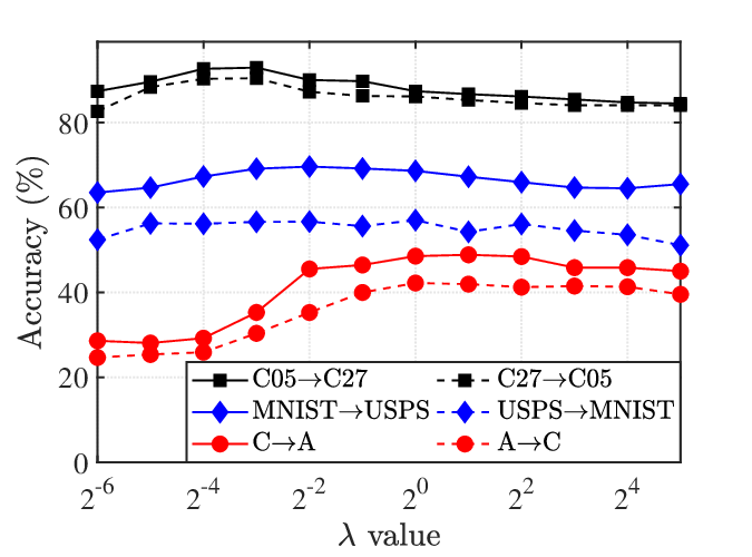
We also analyzed the parameter sensitivity of JPDA on different datasets to validate that a wide range of parameter values can be used to obtain satisfactory performance. Two main adjustable parameters, the trade-off parameter $\mu$ and the regularization parameter $\lambda$, were studied. The results are shown in Fig. 5. JPDA is robust to $\mu$ in $[0.001,0.2]$ and $\lambda$ in $[0.01,10]$.

Next, we conducted ablation study to check if the discriminative MMD $\mathcal{M}_{D}$ can indeed improve the discriminability in the target domain, i.e., with $\mathcal{M}_{D}$ (DJP-MMD) and without $\mathcal{M}_{D}$ (JP-MMD, which only considers the transferability). The joint MMD was also used as a baseline. When embedded in DA, the average classification accuracies of the three MMDs are shown in Fig. 6. On average, JP-MMD outperformed the joint MMD, and DJP-MMD, which further considers the discriminability, achieved the best classification performance.

References

- [1] S. J. Pan and Q. Yang, “A survey on transfer learning,” IEEE Trans. on Knowledge and Data Engineering, vol. 22, no. 10, pp. 1345–1359, Oct. 2009.
- [2] S. J. Pan, I. W. Tsang, J. T. Kwok, and Q. Yang, “Domain adaptation via transfer component analysis,” IEEE Trans. on Neural Networks, vol. 22, no. 2, pp. 199–210, Feb. 2011.
- [3] B. Gong, Y. Shi, F. Sha, and K. Grauman, “Geodesic flow kernel for unsupervised domain adaptation,” in Proc. IEEE Conf. on Computer Vision and Pattern Recognition, Providence, Rhode Island, Jun. 2012, pp. 2066–2073.
- [4] C.-A. Hou, Y.-H. H. Tsai, Y.-R. Yeh, and Y.-C. F. Wang, “Unsupervised domain adaptation with label and structural consistency,” IEEE Trans. on Image Processing, vol. 25, no. 12, pp. 5552–5562, Sep. 2016.
- [5] M. Long, H. Zhu, J. Wang, and M. I. Jordan, “Deep transfer learning with joint adaptation networks,” in Proc. 34th Int’l Conf. on Machine Learning, Sydney, NSW, Australia, Aug. 2017, pp. 2208–2217.
- [6] J. Zhang, W. Li, and P. Ogunbona, “Joint geometrical and statistical alignment for visual domain adaptation,” in Proc. IEEE Conf. on Computer Vision and Pattern Recognition, Hawaii, Jul. 2017, pp. 1859–1867.
- [7] H. Lu, C. Shen, Z. Cao, Y. Xiao, and A. van den Hengel, “An embarrassingly simple approach to visual domain adaptation,” IEEE Trans. on Image Processing, vol. 27, no. 7, pp. 3403–3417, Jul. 2018.
- [8] H. He and D. Wu, “Transfer learning for brain-computer interfaces: A Euclidean space data alignment approach,” IEEE Trans. on Biomedical Engineering, 2020, in press.
- [9] R. Gopalan, R. Li, and R. Chellappa, “Domain adaptation for object recognition: An unsupervised approach,” in Proc. Int’l Conf. on Computer Vision, Barcelona, Spain, Nov. 2011, pp. 999–1006.
- [10] M. Long, J. Wang, G. Ding, J. Sun, and P. S. Yu, “Transfer feature learning with joint distribution adaptation,” in Proc. IEEE Int’l Conf. on Computer Vision, Sydney, Australia, Dec. 2013, pp. 2200–2207.
- [11] H. W. Ng, D. Nguyen, V. Vonikakis, and S. Winkler, “Deep learning for emotion recognition on small datasets using transfer learning,” in Proc. ACM Int’l Conf. on Multimodal Interaction, Seattle, Washington, Nov. 2015, pp. 443–449.
- [12] D. Wu, “Online and offline domain adaptation for reducing BCI calibration effort,” IEEE Trans. on Human-Machine Systems, vol. 47, no. 4, pp. 550–563, Sep. 2017.
- [13] D. Wu, V. J. Lawhern, W. D. Hairston, and B. J. Lance, “Switching EEG headsets made easy: Reducing offline calibration effort using active wighted adaptation regularization,” IEEE Trans. on Neural Systems and Rehabilitation Engineering, vol. 24, no. 11, pp. 1125–1137, 2016.
- [14] A. Gretton, K. M. Borgwardt, M. J. Rasch, B. Schölkopf, and A. Smola, “A kernel two-sample test,” Journal of Machine Learning Research, vol. 13, no. 3, pp. 723–773, Mar. 2012.
- [15] Z. Ding, S. Li, M. Shao, and Y. Fu, “Graph adaptive knowledge transfer for unsupervised domain adaptation,” in Proc. 15th European Conf. on Computer Vision, Munich, Germany, Sep. 2018, pp. 37–52.
- [16] J. Wang, W. Feng, Y. Chen, H. Yu, M. Huang, and P. S. Yu, “Visual domain adaptation with manifold embedded distribution alignment,” in Proc. 2018 ACM Multimedia Conf. on Multimedia Conf., Seoul, Republic of Korea, Oct. 2018, pp. 402–410.
- [17] M. Ghifary, W. B. Kleijn, and M. Zhang, “Domain adaptive neural networks for object recognition,” in Proc. Pacific Rim Int’l Conf. on Artificial Intelligence, Queensland, Australia, Dec. 2014, pp. 898–904.
- [18] H. Yan, Y. Ding, P. Li, Q. Wang, Y. Xu, and W. Zuo, “Mind the class weight bias: Weighted maximum mean discrepancy for unsupervised domain adaptation,” in Proc. IEEE Conf. on Computer Vision and Pattern Recognition, Honolulu, Hawaii, Jul. 2017, pp. 2272–2281.
- [19] Y. Ganin, E. Ustinova, H. Ajakan, P. Germain, H. Larochelle, F. Laviolette, M. Marchand, and V. Lempitsky, “Domain-adversarial training of neural networks,” Journal of Machine Learning Research, vol. 17, no. 1, pp. 2096–2030, May 2016.
- [20] J. Wang, Y. Chen, S. Hao, W. Feng, and Z. Shen, “Balanced distribution adaptation for transfer learning,” in Proc. Int’l Conf. on Data Mining, New Orleans, LA, Nov. 2017, pp. 1129–1134.
- [21] X. Chen, S. Wang, M. Long, and J. Wang, “Transferability vs. discriminability: Batch spectral penalization for adversarial domain adaptation,” in Proc. 36th Int’l Conf. on Machine Learning, Long Beach, CA, Jun. 2019, pp. 1081–1090.
- [22] Y. Cao, M. Long, and J. Wang, “Unsupervised domain adaptation with distribution matching machines,” in Proc. 32nd AAAI Conf. on Artificial Intelligence, New Orleans, Louisiana, Feb. 2018, pp. 2795–2802.
- [23] S. Ben-David, J. Blitzer, K. Crammer, and F. Pereira, “Analysis of representations for domain adaptation,” in Proc. Advances in Neural Information Processing Systems, Vancouver, B.C., Canada, Dec. 2007, pp. 137–144.
- [24] B. Quanz and J. Huan, “Large margin transductive transfer learning,” in Proc. 18th ACM Conf. on Information and Knowledge Management, Hong Kong, Nov. 2009, pp. 1327–1336.
- [25] C. M. Bishop, Pattern Recognition and Machine Learning. New York, NY: Springer, 2006.
- [26] G. Griffin, A. Holub, and P. Perona, Caltech-256 object category dataset. Caltech: Technical report, 2007.
- [27] L. v. d. Maaten and G. Hinton, “Visualizing data using t-SNE,” Journal of Machine Learning Research, vol. 9, pp. 2579–2605, Nov. 2008.