A Machine Learning Approach to Adaptive Robust Utility Maximization and Hedging
Abstract
We investigate the adaptive robust control framework for portfolio optimization and loss-based hedging under drift and volatility uncertainty. Adaptive robust problems offer many advantages but require handling a double optimization problem (infimum over market measures, supremum over the control) at each instance. Moreover, the underlying Bellman equations are intrinsically multi-dimensional. We propose a novel machine learning approach that solves for the local saddle-point at a chosen set of inputs and then uses a nonparametric (Gaussian process) regression to obtain a functional representation of the value function. Our algorithm resembles control randomization and regression Monte Carlo techniques but also brings multiple innovations, including adaptive experimental design, separate surrogates for optimal control and the local worst-case measure, and computational speed-ups for the sup-inf optimization. Thanks to the new scheme we are able to consider settings that have been previously computationally intractable and provide several new financial insights about learning and optimal trading under unknown market parameters. In particular, we demonstrate the financial advantages of adaptive robust framework compared to adaptive and static robust alternatives.
Keywords: adaptive robust control, Gaussian process surrogates, portfolio optimization
1 Introduction
Stochastic control formulations have been a core tool in financial mathematics for over 40 years. One fundamental challenge in applying stochastic models to practice is the issue of model risk, i.e. calibrating system dynamics to real life. In this article by “model risk” we mean uncertainty about the underlying probability measure representing the mis-specification between the assumed dynamics and the true probabilistic structure. More precisely, the uncertainty concerns some parameters , so that we have the parameterization . Parameter uncertainty arises in any application, since the required model calibration necessarily leaves some residual inference error about the true parameter values. For example, in problems involving risky assets such as stocks, asset return and volatility are the two main parameters driving the investment decisions, but are notoriously difficult to calibrate.
As one remedy, there have been recently multiple proposals on robust extensions for the underlying stochastic control formulation. The basic strategy is to take a worst-case view among a collection of potential ’s. In the financial context, this conservative perspective stemming from unknown parameters is tempered by the idea of learning the dynamics. Historical data about the risky asset evolution can often be used to improve estimates about its drift and/or volatility. Combining these two concepts of robustness and learning, we adopt the adaptive robust framework recently proposed in Bielecki et al. [9]. This paradigm elegantly connects static robust approaches that do not allow belief updating with adaptive control that fully incorporates the latest estimate within a fixed-parameter setup. Because adaptive control ignores dynamic updating, it is time-inconsistent. However, adaptive robust control also presents formidable numerical challenges as it features an expanded, multi-dimensional state space and non-trivial nonlinear optimization to find the optimal feedback control and the value function . As a result, closed form solutions are ruled out, and standard PDE methods are not feasible beyond the most simple settings.
In this paper we propose and develop a novel algorithm for adaptive robust control. Our approach belongs to the class of Regression Monte Carlo (RMC) and Control Randomization (CR) strategies [10, 5, 12, 14, 26]. The key idea is to recursively construct a functional approximation which is then evaluated over a stochastic (non-gridded) mesh. However, in the context of robust control, existing techniques run into the double challenge of: (i) strong path-dependence of optimal on the control, preventing direct application of Regression Monte Carlo (see Section 4); (ii) the nested optimization due to considering multiple ’s is computationally intensive and requires proper approximation architecture to extract . We employ machine learning techniques to overcome the above challenges, by constructing a non-parametric value function approximation [21, 7]. Specifically, we leverage tools from statistical emulation in Stochastic Simulation [11, 6] (and more broadly the Design and Analysis of Computer Experiments field [25]) by recasting the task of solving the Bellman equation as a statistical learning problem of fitting a surrogate (i.e. a statistical model) for [23, 18]. Our framework resembles recent results for Monte Carlo based solvers of Hamilton-Jacobi-Bellman equations [16, 2, 13]. However, unlike the above references that propose to apply Deep Neural Networks (DNN) for the function approximation step, we rather rely on Gaussian Progress (GP) surrogates. GPs is a core machine learning technique which is well-suited for cases where simulation is expensive and therefore efficient surrogate training is needed (in contrast, DNNs are best suited for high-dimensional problems where maximum flexibility is needed and a lot of training data is available). Related use of GPs is in [3, 18].
Utilizing our numerical algorithm, we provide an extensive investigation into the adaptive robust approach to optimal investment and nonlinear hedging. These are two fundamental problems in financial modeling, yet few fully numerical algorithms have ever been available. Our analysis provides new insights into the interplay between robustifying beliefs, learning and investing/hedging. In particular, we investigate the dependence of the conrols and the terminal wealth on risk- and robustness-level parameters.
The rest of the paper is organized as follows. The rest of Section 1 sets up the adaptive robust formulation and lays out the associated discrete-time Bellman recursions. Section 2 develops our numerical methodology and the Gaussian Process surrogate-based algorithm. The second half of the paper illustrates the algorithm on an Optimal Investment (Section 3) and Hedging (Section 4) case studies. Finally, Section 5 provides discussion on the numerical aspects and concludes with a list of additional enhancements.
1.1 The Adaptive Robust Bellman Equation
Let be a measurable space and a fixed time horizon. Let be the discrete time set and be a non-empty set, which plays the role of the global parameter space, so that for each there is a probability measure on . We write to denote the expectation operator corresponding to . We consider a controlled stochastic Markov state process taking values in the state space . We postulate that this process is observed, and we denote by its natural filtration. The optimization problem involves the family of admissible feedback control processes, which are –adapted processes defined on with taking values in a measurable space and being the feedback control applied at time .
Consider the objective of maximizing a reward functional
with running rewards and terminal reward . In the two financial motivations we have , but since our algorithm is of independent interest, we continue with this slightly more general setup. In the classical setup, the dynamics of are described through a probability measure and dynamic optimization of is reduced to the classical dynamic programming Bellman equation
| (1) |
with and .
The pervasive challenge of prescribing -dynamics implies model mis-specification for determining . Robust control injects consideration of multiple models directly into the optimization step (1) via a generic min-max formulation. Therefore, the single is replaced with many ’s. In the parametric setup we consider, model uncertainty is indexed via whose effect is through the dynamics
| (2) |
The mapping captures the joint effect of the initial condition , the control applied at epoch , the parameterized measure , the stochastic shock and the time-dependence . Note that (2) postulates that we may re-write the evolution of in terms of external, model-independent stochastic shocks; in the common setting we consider, are independent and identically distributed random variables (without loss of generality taken to be standard Gaussian in some ).
The robust control setup then includes an intermediate worst-case optimization over a collection , of measures:
| (3) | ||||
| (4) |
where is the density of the random variable . The expression (3) can be seen as a min-max game between nature that picks and the controller who counteracts with her control . In information-theoretic language, (3) is a game against the adversary who selects a probability measure among the Knightian uncertainty set [15]. Note that the adversarial parameter set is understood to be dynamic, i.e. is adapted to the information available by period and in particular can depend on .
The adaptive robust control as developed by Bielecki et al. [9], couples the Bayesian updating procedure to the set of measures in (3). Specifically, we take
re-interpreted as the robustified belief set defined by the latest estimate . As a canonical example, is the posterior credible interval at some level (say the 95% CI) centered around the unbiased point estimate . This interpolates dynamic adaptive control, where (no uncertainty but learning), with the robust versions that do not allow for learning, independent of . (We should also mention the myopic adaptive formulation where one plugs-in into the static model that treats as a parameter. This is in fact the most common applied usage which myopically separates learning from control.)
The learning algorithm is meant to reduce the uncertainty about the true probabilistic structure driving . If one assumes that there exists such that for all and the learning and estimation are asymptotically perfect, as then it is also reasonable to expect and the adaptive robust method brings a consistently conservative extension of Bayesian adaptive control. However, the framework can also handle more general situations, such as when never converges to a singleton, or when no exists. Thus, the adaptive robust can handle non-stationary models where the dynamics change over time (as might be imagined happens in real markets, leading to a process ); in such settings represents the best current guess about . So the size of need not go to zero.
Returning to the control objective, since now affects the inner optimization in (4), it is augmented to the system state
The dynamics of consist of the autonomous dynamics of , as well as the filtering equations that govern the evolution of . We summarize them by the mapping
which aggregates the previous dynamics of the state process with the filtering equations for . Note that those joint dynamics are degenerate since a single noise term simultaneously drives both and . As a result, there is a strong dependence between and , and more generally , which is to be contrasted with the static robust framework where and are independent. The resulting adaptive robust Bellman equation which is the main object of analysis in this article is then
| (5) |
Note that now simply denotes expectation over which is the sole stochastic, model-independent component above; the parameter dependence and model risk are encoded in . The solution entails applying backward induction over to compute .
1.2 Solving the Bellman Equation
To implement the adaptive robust framework, we must solve (5) which practically reduces to (4) with the state-dependent uncertainty set as in (13). If we define the operators via
then the discrete time Bellman recursion is . is the propagation operator that computes the continuation value based on taking conditional expectations of step-ahead value function. is the optimization operator that computes the optimal control at , recording the optimizers . is the worst-case parameters (i.e. beliefs) for the model dynamics given and is the robustified feedback control in state . The difference vs is precisely the precaution taken by the controller against model mis-specification.
Three challenges must be handled to solve (5):
- •
Continuous state space: because the state space of is continuous and multi-dimensional, some discretization is required to handle it computationally. This discretization however implies that (i.e. ) will not be computed for all potential , but only for some finite subset. Therefore, space discretization must be accompanied by interpolation in order to be able to evaluate for arbitrary in subsequent steps.
- •
Integration: the integral over in (4) requires approximation given that the integrand is not analytically available. This implies that the true conditional operator is to be replaced with an approximation , i.e. is replaced with .
- •
Optimization: finding the optimizers and is generally not possible analytically, so another approximation is required to carry out these optimizations numerically. This implies that we replace with an approximation .
In low dimensions, the standard technique for Bellman equations are PDE-based solvers that discretize . However, the augmentation of beliefs to the -state necessarily leads to multi-dimensional setups, essentially ruling out PDE-based strategies that are practical only in dimension . At the same time, simulation-based strategies from conventional regression Monte Carlo are also difficult to apply to (5):
- •
The control intrinsically affects the evolution of the state and hence prevents direct simulation of the overall as is done in the standard RMC paradigm.
- •
Parametric representation of (e.g. in terms of polynomials in ) is challenging in dimension and brings the concern of overfitting/underfitting;
- •
Because we face the additional step of inner optimization over , the representation of is critical to yield financially reasonable/accurate estimates of , which is another limitation of classical parametric approximations;
- •
One usually learns by constructing a grid of -values (akin to finite-difference approaches for PDEs); however such gridding is extremely inefficient for and essentially impossible for .
As a result, fully numerical approaches to robust stochastic control have been traditionally viewed as intractable and there remains a large gap in actual use of robust models for financial modeling. In this article we resolve these challenges, making contributions along two directions. On the algorithmic side, we propose a new, machine-learning-inspired algorithm for (4). The key concept is to employ a non-parametric value function approximation strategy [21, 7], namely a Gaussian process surrogate. In addition, we borrow concepts from the Design and Analysis of Computer Experiments field [25]) to construct the underlying stochastic meshes. This methodology is quite general, and could also be easily modified to tackle other robust control formulations (e.g strong robust), and other contexts (e.g robust optimal stopping). Moreover, it mitigates the issue of scalability to higher dimensions. Related extensions would be treated in separate sequels, and we see a lot of further potential for such blending of RMC and machine learning. On the finance side, we present two detailed case studies of using adaptive robust paradigm in optimal investment and loss-based hedging. In particular, the latter problem (33) was essentially out of reach until now. Employing our algorithm, we are able to give a comprehensive investigation of the resulting strategy and its sensitivity to different model parameters. We also demonstrate that the adaptive robust framework outperforms the common (simpler) alternatives of static robust and adaptive control.
1.3 Motivation: Adaptive Robust Optimal Investment
The problem of optimal investment in risky financial instruments dates back to Markowitz and Merton and has been extensively studied over the past 50 years. Asset return and volatility are the two main parameters driving the investment decisions, but are notoriously difficult to calibrate. Therefore, there is strong interest in methods that explicitly take into account parameter uncertainty, while allowing one to partially learn asset dynamics.
Let be the constant risk-free interest rate. We assume a fixed time grid . The excess log-return of a risky asset between and is Gaussian with mean and variance . Both and are treated as unknown, yielding the framework of (3) with . Thus, the dynamics of the controlled wealth process under are given by
| (6) |
where is the proportion of portfolio wealth invested in the risky asset. Above we restrict the investor from shorting or leveraging her risky position. The objective is to maximize expected utility of terminal wealth
for a utility function . The augmented state is three-dimensional: and the Bellman equation for is
| (7) | ||||
| (8) |
where the expectation is over the standard Gaussian increment .
To specify the transition map , we recall the learning of the asset dynamics. Given past observations of , the respective MLE estimators are denoted by and under satisfy for the recursions [8]
| (9) | ||||
| (10) |
Note that the above are time-dependent, capturing the idea that learning slows over time as the information set grows. As increases, the weight of the prior rises and the role of the latest shock declines.
In sum, the dynamics of under are prescribed by (6)-(9)-(10), all driven by the 1-D exogenous factor . They are summarized by the map
| (11) |
where are treated as external parameters.
Assuming there is a true , the uncertainty set is described through the (1-)-confidence region for for some confidence level . In the case where only the drift is uncertain and is given, is an interval centered on ,
| (12) |
where denotes the -quantile of a standard normal distribution. In the 2-D case where both and are uncertain, it is shown in [8] that the -confidence region for at time is an ellipsoid given by
| (13) |
where is the -quantile of the distribution with two degrees of freedom.
2 Methodology
Our algorithm is based on value function approximation. This is achieved by evaluating the right hand side of (5) at a collection of inputs and then constructing a statistical surrogate for . Thus, we use a machine learning tool, namely Gaussian Process surrogate [22], to learn based on training data , where , see below. To compute the expectation in (14) is approximated with a quantized sum, and the inner saddle-point is computed locally using a nonlinear optimization algorithm. More precisely we use a numerical quadrature representation of the integral over and a nested fminbnd call to get which is interpreted as the estimated optimal control at . Picking the collection is known as experimental design.
The overall solver consists of a fit–predict–optimize loop over time based on the recursion
| (15) |
where predict is needed to evaluate and fit is to construct . For the latter, we evaluate the right hand side of (15) at which yields the pointwise . Because the latter is based on multiple approximations, including approximating the true , approximating the true saddle-point, approximating the true , we treat them as noisy versions of and thus the surrogate fitting step includes smoothing, rather than solely interpolation. Similarly, we view as pointwise samples from the feedback control map that is also obtained via (an independent) surrogate fitting.
Our algorithm returns the fitted surrogates and for each time step. The interpretation of is as the value function of the underlying adaptive robust control problem. However, for practical purposes we typically wish to know the strategy and resulting utility based on a fixed measure , while (3) assumes that the parameters are dynamically and adversarially drawn from at each time-step. To this end, we concentrate on the outputted feedback control surrogate . To evaluate the resulting utility, we rely on forward Monte Carlo, i.e. we generate out-of-sample forward paths by drawing -realizations based on that induces the controlled trajectories and then evaluate the Monte Carlo estimate
Observe that can also be written as an expectation, but under the path-dependent, “pasted” measure which is defined in terms of the worst-case beliefs at each time step and does not admit a simple interpretation. Indeed, the expectation of is carried out with respect to which depends on . For this reason, the representation is generally not practically relevant.
Remark 2.1.
For an arbitrary , we distinguish between the actual minimizer that is obtained by calling predict to evaluate and then optimizing, and the surrogate-based that is obtained from a statistical prediction. Because optimization is expensive, it is much faster to utilize . We also stress that both and are defined based on and hence will necessarily differ from the true optimal feedback due to error back-propagation.
Remark 2.2.
When the optimization over is over a compact space such as , an alternative to generic fminbnd or optim gradient-free solvers is to employ direct search over a discrete candidate set such as . This is faster but of course introduces a fixed discretization error relative to the true optimum. Conversely, the surrogate can output the gradient that could be combined with the chain rule to enable gradient-based optimization.
Before proceeding to discuss the details of operationalizing the above method, we summarize the original proposal of Bielecki et al. [9] that relied on a Control Randomization (CR) + Regression approach. Bielecki et al. started with a Monte Carlo-based paradigm that works with trajectories of and exploited the fact that the underlying state is an autonomous process. In their approach, one begins by generating trajectories of . In addition, one fixes a measure and uses the above trajectories to construct the corresponding filtered posterior estimates as in (9)-(10). Note that is picked arbitrarily and serves as a “baseline” probability measure like in the CR method [1, 17]. Next, the Bellman equation (3) is solved pathwise along the above as follows. Given , one solves for by replacing the integral with a weighted sum
| (16) |
where the Gaussian quadrature recipe specifies the appropriate knots and corresponding quadrature weights . The latter are optimized to minimize a certain global criterion [4, 20]. Since the noise distribution is fixed throughout, the optimal quadrature recipe is pre-computed and stored offline. In the second sub-step, the one-step-ahead values are approximated—since they will not fall on the mesh —through linear interpolation of the training collection .
The above recipe has several limitations that our new proposal overcomes. First, the use of a pre-specified leads to a non-adaptive experimental design, which puts potentially very far from the likely values of (depending on whether is “good” or not). By breaking up the path-based construction, we are able to adaptively build better designs, which in particular leverage the structure of . Second, linear interpolation of ’s brings three restrictions: (i) it poorly scales in dimension , because the interpolation requires sorting of all the sites to identify nearest neighbors; (ii) it implies that is piecewise linear which a restrictive approximation architecture (in particular non-smooth which may cause problems when solving for ); (iii) it takes the estimated values of are taken as exact, providing no ability to smooth previous approximations. Third, the procedure only outputs the pointwise estimates ; there is no simple way to obtain for arbitrary , essentially ruling out out-of-sample estimation under any other measure than . Fourth, the approach has no way to avoid extrapolation when using (16); linear extrapolation is prone to significant errors that are likely to back-propagate. Fifth, pre-simulation under requires to use the same mesh size across all time steps.
2.1 Gaussian Process Surrogates
Gaussian process models is a popular choice for flexible statistical models. They allow a consistent treatment of interpolation and regression with very few tunable hyperparameters. The idea of GPs is to view the function to be approximated as a realization of a Gaussian random field with covariance kernel . Training the model then reduces to applying the Gaussian conditional equations, i.e. evaluating the distribution of the random field given the data. The Gaussian structure implies that the conditional process is still Gaussian, so its distribution is summarized through the posterior mean and posterior (co-)variance , interpreted as the model-predicted approximation and the corresponding posterior uncertainty or “standard error”.
Intuitively, the GP offers a methodology to put a smooth surface through the data labelled generically as . For numerical stability, we introduce the “nugget” , so that rather than exactly interpolating the given ’s, the surrogate also smoothes. Namely, the nugget is equivalent to assuming
In our context, adding ’s is justified via the errors coming from quantization and numerical optimization and we use . The predicted at any input is given by
| (17) | ||||
| with corresponding posterior covariance | ||||
| (18) | ||||
with the vector and matrix defined by
| (19) |
Above is a identity matrix and is the noise matrix.
To construct a GP surrogate requires selecting a kernel family and the corresponding hyper-parameters. The latter step is typically done through Maximum Likelihood Estimation, i.e. a nonlinear optimization problem involving the respective likelihood of observations. A common kernel family we use is the Matern-5/2,
| (20) |
where the lengthscales and the process variance are estimated via maximum likelihood. Specifically, we use the GPML Matlab package to obtain the MLE for the hyperparameters . Another kernel is the squared-exponential
| (21) |
The GP predictive surface is akin to kernel regression in the sense that the prediction (17) at is always a weighted average of the ’s, with the weights driven by the spatial covariance structure encoded in . In particular, if the spatial correlation decays quickly, the surface will tend to be more “bumpy”, while for very strong spatial correlation the surface will be nearly flat/linear. The differentiability of the predictive surface is driven by the properties of . Under the Matern-5/2 choice (20), the resulting is twice-differentiable, while for (21) it is . In both families, the lengthscales determine the spatial “wiggliness” of the fitted surface in the respective coordinate. Note that different lengthscales (anisotropy) in different coordinates allow for to be, say, more flat in , but more flexible in .
For the propagation operator showing in the Bellman equation we proceed as in (16), approximating the integral over a standard normal distribution by a -points optimal quantizer , i.e. a discrete sum over quadrature points .
Remark 2.3.
In CR-RMC [1, 17], solving the Bellman equation
is handled by defining the q-value across , building a surrogate and then finding as the analytic maximizer of . In contrast, in our approach, we first fix and maximize at to obtain , then fit a surrogate , effectively reversing the order of optimization and emulation.
2.2 Experimental Design
The quality of the regression estimates is critically linked to the choice of the simulation design . Specifically, accuracy of the GP-based at some given input is directly related to the density of the design around . This is the localization property of the GP and matches the intuition of constructing an interpolant for the training data : the interpolated prediction would be good in the neighborhoods of ’s, and progressively worse far away. In particular, as gets far from the training inputs , the GP prediction is driven by the chosen asymptotes of reflecting extreme extrapolation. Specifically, for GPs we have that reverts to its prior mean.
Based on the above discussion, the design should concentrate on the region of interest. In our context, the latter is driven by the pairs that are likely to be encountered by the controller at step . In addition, since the key output we seek is the investment strategy , the hardest learning task is to identify the optimal control when the constraints are not binding. Consequently, the region of interest is .
Another problem that requires attention is extrapolation in estimating the surrogate . Extrapolation tends to lead to large estimation errors in approximating the true conditional expectation operator . With this in mind, we need to select the design so that extrapolation is minimized. In order to compute , we must consider at any within . This, in turn, means that we need good estimation of , , where recall that comes from Gaussian quantization. Figure 1 displays the relationship between and the set of all next-step locations . These are the locations where we must evaluate and hence highlights to what extent the method requires extrapolation. On the right panel we compare all needed predictive sites against the used for training .
Given a region of interest , there are two main concepts to generate a training set that targets . The first idea is a “density-based” approach that aims to make mimic the distribution of under . Recall that includes the exogenous and the path-dependent . One method to handle this path-dependency is based on Control Randomization [1, 17] which was also the motivation for generating the path-simulations in Bielecki et al. [9]. We first pick some and generate paths under . In other words, we pick some “true” model parameters (e.g. using the prior mean estimates ) that are used to generate . A collection of such independent “pilot” paths can be then used to set .
The second concept is to apply space-filling schemes which aim to yield a “uniform” sample from the region of interest. This approach is similar to classical maximin/max-entropy experimental designs in statistics. Space filling is achieved by specifying an input domain (usually some polyhedral or rectangular bounding box) and then a space-filling sequence. A popular choice are Quasi Monte Carlo (QMC) sequences that are used as a variance reduction tool to ensure that does not contain any “holes” that might degrade estimation in their neighborhoods. A QMC sequence offers a deterministic way to sequentially fill the unit hypercube and can be straightforwardly scaled and clipped to fill any polyhedral domain. For example, Sobol QMC sequences offer a discrete of any size .
In Figure 1, we show an adaptive “mixture” design that we utilize for the portfolio optimization problem with unknown . It is obtained in three steps. In the first step, we simulate forward paths under a pre-specified that yield . We then utilize these “pilot” paths to obtain a convex hull . In the second step, we utilize the Sobol QMC sequence to fill the respective with sites. Finally, in the third step, we augment with another sites based on , i.e. add new sites where the control was non-trivial in the previous time-step.
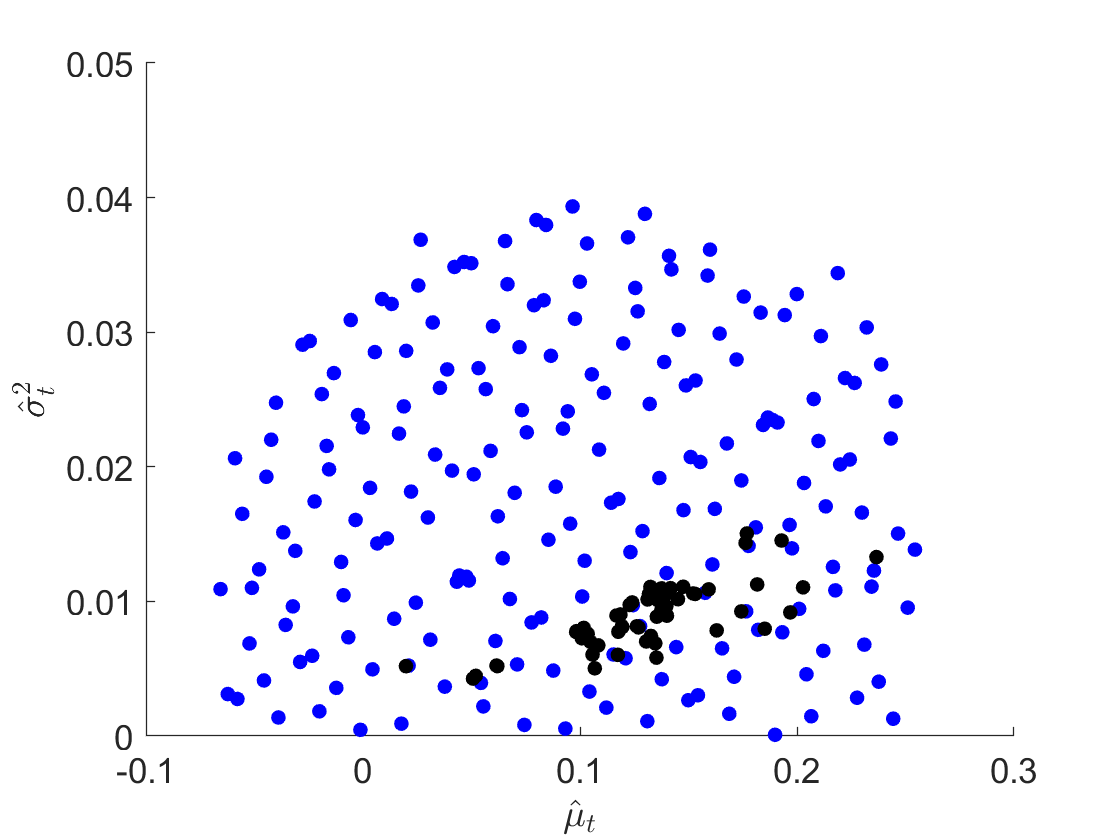
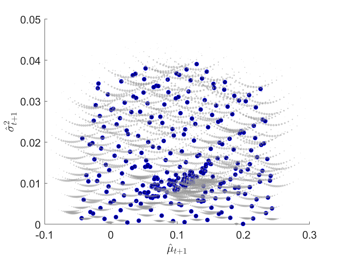
Remark: Given the complexity of (5) which requires solving a min-max problem at each design site , it is not computationally feasible to have thousands of ’s. Already for a rather small design like in Figure 1, we are looking at more than a million of predict calls to the GP surrogate each time step ( for each integral, multiplied by about 60 optimization steps to converge to the min-max optimal value, multiplied by design sites). This is a principal reason why we advocate Gaussian Process surrogates which excel in learning from small-to-moderate designs. Note that GPs are still computationally intensive and their speed is very sensitive to , which is the reason for all the above care in building a good experimental design. While a linear surrogate that utilizes ordinary least squares regression with a pre-specified set of basis functions is much faster, its rigid structure performs terribly for learning ; in our experience success of the algorithm hinges on having enough degrees of freedom. Other alternatives for value function approximation besides GPs are left for future research.
2.3 Algorithm
Algorithm 1 summarizes our procedure. It further makes a slight extension to allow for time-dependent design size . The second Algorithm 2 evaluates the performance and strategy of the controller under some test measure utilizing a forward Monte Carlo average over fresh paths. The actual simulations are under where can vary across paths or even across time. For example, if we take uniformly, then we mimic the static robust setup. The resulting out-of-sample estimator is guaranteed to be a lower bound for since it is directly based on the suboptimal strategy and its only error is the Monte Carlo averaging due to the finiteness of .
| (22) |
| (23) |
To summarize, the proposed framework organically integrates the construction of and with the paradigm of Design and Analysis of Computer Experiments that views the intermediate step as inference of an expensive black-box function. The adaptive ’s target the learning of the optimal control, while the GP setup captures the spatial borrowing of information to predict without directly optimizing. Their combination improves efficiency, scalability, and interpretability, and should be contrasted to the conventional implementation where is a grid and the approximation architecture is a linear interpolant (piecewise linear ). Our algorithm is also highly modular, allowing additional ways of approaching the aforementioned sub-problems of numerical integration and numerical optimization. Intuitively, the computation revolves around repeated optimization, and our framework achieves substantial gains by leveraging already obtained solutions of similar optimization problems, in analogy to parametric optimization. To our knowledge, we are the first article to propose this strategy for robust stochastic control.
Remark 2.4.
In the case studies below we have and the GP surrogate tends to over-smooth in regions where or as it does not like flat responses. We regularize the constraint by carrying out optimization of over a larger domain . The relaxed maximizer is then fed into the GP representation of the optimal control, and the resulting prediction is projected as . This regularization makes sure that the data used to build the surrogate are smooth and do not have the non-smooth cut-offs at 0 and 1. In the first example below we take .
2.4 Algorithm Stability
The overall algorithm complexity can be broken down into the overhead of fitting the surrogates and the cost of calling predict during the Bellman recursions. With a GP surrogate, the complexity of model fitting is at each time step, so total. Each GP prediction requires effort and is employed times during each evaluation of the conditional expectation and in turn is called times (which is state-dependent) by the nested optimizer that is solving for . Overall, we obtain complexity for Algorithm 1. Similarly we have complexity for generating forward paths to obtain the out-of-sample evaluation of in Algorithm 2.
An important aspect is that the proposed algorithm is non-deterministic since the outputted and depend on the underlying random samples of . Recall that affects the that is used for the surrogate fitting. In the GP context, this will modify both the GP hyperparameters, as well as the actual prediction since shows up on the RHS of (17). Therefore, running the algorithm twice will generate slightly different fits. The respective variance would be amplified if the simulation designs are also random (e.g. dependent on the pilot paths as in our setup) since then also the ’s would vary from run to algorithm run. Yet another increase in algorithm variance would occur if also the conditional expectation is approximated via Monte Carlo rather than Gaussian quadrature.
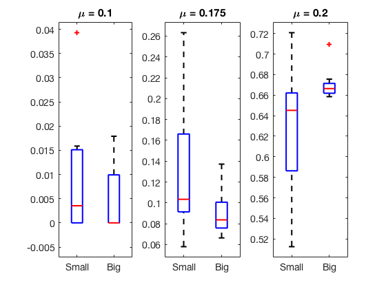
In this vein, the design size plays a double role of (i) decreasing the above macro-replication variance through Law of Large Numbers with respect to ; (ii) increasing accuracy (i.e. reducing bias) by raising the fidelity of and (i.e. reducing functional approximation error between the surrogate and the true minimizers/value function). Figure 2 displays a boxplot of across algorithm macro-replications when using vs . As expected, a larger design reduces overall variance, as well as the bias. To illustrate the role of another tuning parameter, we show the impact of the quantization level on the accuracy of the results.

3 Adaptive Robust Utility Maximization
In this section we illustrate our algorithm from Section 2.3 for the task of portfolio optimization under uncertain drift and volatility. The full list of parameters is listed in Table 1. We present two different case studies.
In this setting, we can simplify the computation of in (22) by dimension reduction. Namely, by monotonicity we take the 1-dimensional infimum in the unknown parameters just over the boundary of the parameter space. Let denote the parameters achieving the infimum of . Switching to polar coordinates it suffices to find and record the corresponding angle using the map
| (24) | ||||
| (25) |
The minimization defining (and hence ) is then done over using the default fminbnd algorithm in Matlab with a tolerance threshold of . Similarly, we use fminbnd to minimize over the scalar control domain .
3.1 Static Investment and Hedging
It is instructive to consider the one-period, aka static version of the optimal investment problem. In this simplified setting, the terminal controlled wealth under is given by
| (26) |
where is the date that trade happens. Above is standard Gaussian in and due to the scaling of the power utility function, we may take without loss of generality . The static optimal investment problem is
| (27) |
with the uncertainty set
| (28) |
Observe that due to the one-period feature, the role of is purely to determine the set of ’s that are being considered. Moreover, without loss of generality we may take the horizon to be fixed, whereby the size of is controlled by the ratio which is interpreted as the measure of robustness. As , , and is the “radius” of adversity.
To solve (27) it suffices to evaluate the map and then find its saddle point (i.e. the location) over the constrained domain and . Due to the concavity of the utility preferences, this map is increasing in and decreasing in . Consequently, the infimum over the robustified beliefs will always be achieved in the NW quadrant, so that and . Therefore we can again switch to polar coordinates reducing to a 2-dimensional function of the control and the angle . For example, means taking the minimum possible drift.


The left panel in Figure 3 shows for a representative pair of initial beliefs in the range . For a fixed investment level , is a convex function with a minimizer . However note that when , is independent of the -dynamics, i.e. is constant in . The respective infimum is then undefined and there is no . The saddle-point is the maximum and is indicated by the red dot on the left panel, where is visualized by the red line. In this particular case, and .
The right panel of Figure 3 displays as a function of the initial beliefs for two different robustness levels. As decreases, gets larger and therefore the worst-case (inner infimum) becomes worse. Consequently, the controller acts more conservatively, i.e. increases in . Otherwise, has the familiar shape of increasing in (asset returns being more favorable) and decreasing in (asset risk rising). Note that when returns are not sufficiently high and/or volatility is too large, the optimal action is , i.e. to invest only in the risk-free bond. This happens in particular when intersects with the negative half-plane, i.e. the investor believes that negative returns are possible.
The left panel of Figure 4 visualizes the structure of the robustified beliefs as a function of . Recall that (quivers pointing to the West) corresponds to the worst-case making as negative as feasible. This is the robustified belief in the middle and top of the state space. In the bottom-right (very high and very low ), the worst-case trades off reduced returns against increased risk. Finally, in the left half of the plot we have , so that there is no (no quivers displayed) since is constant. In that case the consistent interpretation is to keep unchanged.


Finally, the right panel of Figure 4 addresses the question of trading constraints. Typically we find that is convex, i.e. has a unique global maximum. In that case we may find the unconstrained global maximum and then constraints of the form translate into . The plot reveals several useful insights. First, we observe the “shrinkage to zero” effect: robust control implies that a risky position will be assumed only if there is a clear understanding regarding . Therefore, if is small, the robust solution is to take . In that sense, shrinks the non-robust control to zero. Because the size of is influenced by the amount of this shrinkage grows in as observed in the plot. Second, we observe that for a fixed is essentially piecewise linear in , capturing the original Merton intuition that is linear in asset returns. Third, we note that leverage and short-selling remain feasible with adaptive robust control provided that the adversarial set is far enough to one side of the half-plane. Thus, we observe in the bottom-left corner (strongly negative Sharpe ratio) and in the bottom-right corner (very high Sharpe ratio). Fourth, we stress that the plot is (roughly) symmetric about which is the risk-free alternative.
3.2 Multi-period Optimal Investment
We now return to the original multi-period setting with time-steps, i.e. and . This setup is very similar to the previous section, except that is now time-dependent. Figure 5 illustrates this dependence by showing a contour-plot of for two different time steps . Recall that at early epochs is larger so ceteris paribus the investor is more conservative and tends to increase in . This is indeed observed in the figure, matching the intuition of “learning-as-you-go”. We note that there are competing effects, in particular due to the time-dependence in the dynamics of (learning slows over time) and the time-dependent effective risk-aversion (the value function becomes less concave as increases).
Structure of Optimal Control: The left panel of Figure 5 shows the optimal feedback control surface . We observe that when is low and monotonically increases as the posterior mean asset return rises. Eventually for high enough , . This structure suggests that we can concentrate the statistical modeling efforts in the intermediate region where since otherwise the corresponding feedback control surface is completely flat and therefore easy to interpolate. The latter fact also implies that even extrapolation is feasible since we just need to ensure that the surrogate is set such that the respective asymptotes in are to the left and to the right.


Structure of Robustified Beliefs: We recall that is only well-defined when , since otherwise the investor is not exposed to returns uncertainty. Therefore, only exists for high enough and low enough (the SE corner of the state space). In the latter region, we find that the principal effect is to decrease the drift rather than to increase volatility, so that . In the multi-period context, low would also hurt the investor, so will also occur at the early time steps.
3.3 Distribution of Terminal Wealth
To obtain an out-of-sample performance metric of the computed investment strategy we apply Algorithm 2 in Section 2.3. For the test measure we use , i.e. static Knightian uncertainty where is drawn from a known prior at and then kept constant through time. To be consistent, we utilize the initial adversarial set . Specifically, for the forward simulations we sample independently and uniformly for . For the discussion below, we took and so the investor starts out under-estimating both the mean returns and the return volatility.
We recall that the classical Merton solution with fixed is time stationary and given by
Using the above we can compare our adaptive robust solution to the following alternative strategies:
- •
Merton strategy based on which is the static robust formulation;
- •
Merton strategy based on which is the adaptive formulation;
- •
Strategy equivalent to our adaptive robust algorithm with () which dispenses with robustness.
For the static robust approach, the worst case of asset dynamics corresponds to a low Sharpe ratio. In particular, for our parameter values, since negative return rate cannot be ruled out , the robust for all , and no investment would be ever undertaken. This point clearly illustrates why learning is desirable, as it allows the investor to overcome initial pessimism (or worry about model risk) through gradual collection of information. If enough favorable information is learned then she will eventually become optimistic enough to invest. At the other extreme, the adaptive case leads to over-confidence and hence over-investment. In particular, the adaptive method generates much larger variance, i.e. risk, in compared to adaptive robust, as the investor trusts her myopic beliefs too much.
Figure 6 shows the distribution of terminal wealth as we vary the risk aversion parameter and the robustness parameter . As expected, less risk averse investors will have higher and therefore larger accompanied by much larger . Similarly, agents that are less conservative (and therefore have smaller ) will tend to again invest more. However, being too “trusting” and not guarding against model mis-specification will eventually hurt wealth accumulation (compare to , so that has a hump shape as a function of ).


4 Adaptive Robust Optimal Hedging
It is of financial and theoretical importance to study optimal hedging problem in an incomplete market setup under model uncertainty. The uncertainty issue was addressed, for example, in the paper [19] where the author used Bayesian estimators in place of the corresponding parameters. We will compare our approach to a similar method that uses maximum likelihood estimators instead. Another standard method widely used among banks when dealing with model risk is the so-called conservative or worst-case approach, and it is in principle the same as the static robust approach.
We denote by the market price process of the stock and we postulate that the increments of are log-normal with parameters :
| (29) |
Dynamic trading strategies are based on a discount bond and the stock , and are represented by a predictable discrete-time process identified with the number of shares invested in the stock from until . The bond investment is then determined from the self-financing constraint. For an admissible we define the corresponding wealth process as
| (30) |
where is the initial endowment, assumed to be fixed and deterministic.
We are interested in dynamic hedging, using an admissible trading strategy, of a European style option written on the stock , maturing at time and with the payoff , where is a measurable function. To address nonlinear hedging, we define the objective as optimization of the hedging error through [24]
| (31) |
where is a positive measurable loss function such that . This setup offers a loss-based criterion that is applicable both in complete and incomplete markets. The main loss function we will consider is of the form
| (32) |
where the constant reflects the relative importance of super- and sub-hedging. When the investor is penalized only for not having enough to cover her liability, while leads to and is the -equivalent of the classical quadratic hedging criterion.
We consider adaptive robust hedging in the context of uncertain asset drift and volatility, leading to a four-dimensional state: which under has the dynamics prescribed by (29)-(30)-(9)-(10). The Bellman equation becomes
| (33) |
We may interpret as the robust expected loss, so that and lower implies better ability to -hedge. For example, in the one-sided example with , will be monotone decreasing in both and .
This setup is conceptually similar to the previous section but presents a harder computational challenge due to its higher dimensionality and the non-smooth relationships between and the state variables. Moreover, it features the fully endogenous wealth process which cannot be reasonably “forward-simulated” without assuming . To overcome this issue we adopt the Control Randomization approach of selecting a measure to build the designs .
For illustration, we henceforth consider a European style Call option written on the risky asset with strike , . The investor is short (sold) the Call and aims to minimize her hedging error starting with initial endowment .
4.1 Implementation Details
For the hedging problem, is four-dimensional, and there is a high correlation between and , so that the design has a certain 3-d structure. Moreover, necessarily there will be a dependence between and wealth . To construct we use a three-step procedure. First, we generate “pilot” forward paths of under . The pilot paths are based on randomized , , as well as initial stock prices , where . Specifically, given we sample initial beliefs , uniformly from and , respectively, as well as around the strike price . Second, we construct a set of augmented pilot sites by adding a few more ’s based on the edges of adversarial beliefs . This step helps us reduce extrapolation when evaluating during Gaussian quadrature. Third, we use a space-filling strategy to fill in “holes”, employing a QMC sequence-based design over the convex hull of the augmented pilot sites at each . This is done by “pulling forward” the design to the next time-step using the map with the empirically sampled ’s and then randomly replacing 100 pilot sites by sites from the respective QMC (Sobol) sequence in . This yields the experimental design , .
Finally, to specify we compute the Black Scholes prices and independently sample . This leads to a “tube” in the plane that contains the Black Scholes prices, with the idea that these are the likely wealth levels (assuming that ) to be visited.
The algorithm described in Section 2.3 is tailored for applying the adaptive robust framework to the optimal hedging problem. For the hedging problem monotonicity of in terms of or no longer holds true. Hence, the supremum is not necessarily attained on the boundary . Nevertheless, we continue to take advantage of the elliptical nature of working in the respective polar coordinates representing the angle and distance from . We then discretize uniformly in terms of and and fixing carry out a direct maximization over the discrete set of adversarial beliefs. This finally yields the robustified parameters :
Minimization of the resulting function
| (34) |
with respect to is done by using fminbnd in Matlab with a tolerance threshold of , where we double-check whether the minimum is achieved at the boundaries . For the super-hedging loss function , we note that when , the expected loss is numerically zero, so that is numerically constant and the maximizer of (34) is ill-defined. This is the scenario where the option can be super-hedged with very high probability so it does not matter what the current hedge is. We found that it helps to detect such cases a priori, setting for them.
 |
 |
 |
Figure 7 shows the estimated angle and distance via a quiver plot at three different time instances . A first observation is that is not trivial as the adversarial beliefs are not necessarily on the boundary. Secondly, in this problem depends both on the current stock price and the current wealth . In the plot we consider at-the-money case and at-the-wealth case . We observe that for early , the worst-case adversarial corresponds to maximizing the stock return , , so as to maximize the Call value. Asset volatility begins to play a more important role as expiration approaches and the Vega/Gamma of the Call increase. As a result, rotates counterclockwise and the worst-case now involves making both and larger. Third, the Figure indicates the impact of on : the distribution of follows the rotation of . Time-dependency of is also illustrated in Figure 8. The optimal strategy is increasing in when is relatively small, and is decreasing when is large for . On the other hand, the hedging strategy in general increases with respect to at . These show the competition between the two factors and at different time steps. At early stages plays a more important part: small causes under-hedge and large leads to over-hedge. When we approach terminal time, is the main driver of the hedging error: higher stock price implies higher projected option payoff, hence one would invest a larger proportion of the wealth into the stock to reduce the hedging error. In addition, change in the region of the contour reflects different experimental designs for different time steps.

4.2 Comparison to Other Approaches
As comparators to adaptive robust control, we consider again the myopic adaptive (MA) and static robust (SR) formulations, as well as a naive adaptive Delta (AD) hedging. The latter buys shares at each step , plugging-in the latest parameter estimates into the classical Delta-hedging strategy of the Black-Scholes model. MA control corresponds to first solving the optimization problem treating as a parameter, which yields . The adopted strategy is then which, like the adaptive Delta, leads to a purely learning-based approach. The SR formulation takes and then solves the Bellman equations (33).


To make the comparison, we compute the distribution of the respective terminal hedging errors on out-of-sample forward paths, using . Figure 9 shows the empirical histogram of from the forward simulations. Better hedging corresponds to lower average loss and in particular should concentrate errors closer to zero, so that and small are preferred. We see in Figure 9 that the hedging error of Adaptive Robust strategy is more concentrated around . In the out-of-the-money and in-the-money cases, Adaptive Delta leads to significantly larger tail on the positive side. Hence, AR produces a comparatively better strategy which “super-hedges” (consistently more negative ) AD. This is not very surprising as the AD recipe is ad hoc and is not targeting the loss function.


| AR | SR | MA | AR | SR | MA | AR | SR | MA | |
|---|---|---|---|---|---|---|---|---|---|
| mean() | -6.09 | -8.82 | -2.79 | -7.11 | -3.34 | -0.60 | -6.81 | -1.01 | -1.26 |
| std() | 16.06 | 5.07 | 21.62 | 5.24 | 19.62 | 25.05 | 5.26 | 24.09 | 22.95 |
| 21.76 | -1.04 | 37.57 | 1.72 | 33.19 | 49.81 | 1.86 | 52.07 | 43.06 | |
| 3.52 | 0.08 | 6.50 | 4.07 | 8.44 | 13.83 | 5.70 | 13.59 | 14.31 | |
Figure 10 shows that the AR approach frequently performs better than SR and MA strategies. When taking a two-sided loss function (), the hedging error of AR concentrates more around zero and has apparent thinner tails on both sides compared to the other two. Due to lack of learning, SR strategies are more “conservative” and over-invest in the underlying asset (see Figure 11 below) which increases the variance of . Myopic adaptive control is over-optimistic and tends to lead to very high variance, already noted in [9]. Table 3 shows the impact of on the performances of these three approaches. SR does better than the other two when . Note that this corresponds to the super-hedging objetive, hence it is not surprising that the conservative approach wins as it over-invests in the risky asset. For where positive hedging error is also penalised, adaptive robust formulation outperforms the other two. Choosing the optimal strategy in these cases are more delicate, and a method which combines learning and robustness handles the situation better.
4.3 Comparison of Optimal Hedges
Compared to hedging strategies generated by other approaches, the adaptive robust strategy follows the movement of the underlying more closely. Such behavior can be understood as a better learning of the model than other methods. Figure 11 displays a sample trajectory of and corresponding across the above three approaches. When stock price is volatile during the time period, robust strategies and are much more stable than the pure learning-based strategies and . It is also worth mentioning that for the static robust approach the assumed drift corresponding to the worst case model is very high. Namely the SR worst case is that the Call ends in-the-money and a large positive hedging error results. To compensate against this scenario, the static robust strategy over-invests in the risky asset to ensure that conditional on , which conversely generates larger risk in other, less adversarial scenarios. This explains why in Figure 11.


5 Discussion
5.1 Enhancements
A central feature of our machine learning approach is the rich set of opportunities to enhance the computations. These concern the ultimate aim of (i) faster running time; (ii) more stable and accurate estimates of and . Practically, we would like to be able to specify a small simulation budget and then obtain good results quickly. We do note that there is a third dimension of actual running time—if the statistical surrogate model is too complicated then its overhead can be high even when is low. For example, we can propose heuristics for sequential, adaptive designs that would maximize the learning ability of as a function of , but actually slow down the algorithm (hence we deem them low-priority extensions).
Faster optimization: Generating a single training pair in (23) requires solving a nested optimization problem (maximizing over , minimizing over ), which is the most expensive part of the algorithm. Since this is done inside all the loops (over and over ), making this step efficient is central to fast performance. In our existing implementation we utilize off-the-shelf gradient-free optimizers (fminbnd and fminsearch in Matlab) which are agnostic to the structure of and and operate completely generically. One way to speed up isthrough warm-starting the optimizers at the location , i.e. assuming that the new optimizer is the same as the one from the previous (later) time-step. For in (22)-(34) we may warm-start the optimizer at . A further enhancement is to rely on gradient-descent optimizers which would require to estimate . Within the GP setup we may analytically differentiate the GP kernel to learn which in turn could be converted into .
GP Hyperparameters: A significant portion of the algorithm running time is spent on fitting the GP surrogates, i.e. inferring (typically by maximum likelihood maximization) the respective hyperparameters . This is a hard nonlinear optimization problem with total time complexity , with the dependence on due to the need to fit a surrogate at each time-step . Generally, the hyperparameters are stable over time, so one could use this for another warm-start in the MLE optimizer, or even directly set , freezing hyperparameters across (some) time-steps. Because the GP surrogate is data-driven, the final prediction depends mostly on the training data and less on the precise value of .
In terms of accuracy, an important piece of building the surrogate are its extrapolation properties. Recall that for extrapolation the GP prediction reverts to its prior outside of the input domain. For fitting the control surrogate in both case studies we take , but other choices would be appropriate depending on the problem/surrogate and in our experience can play a nontrivial role in ultimate solution quality. (However, note that is only relevant for extrapolation—within the prediction is driven by the training data.)
5.2 True Monte Carlo
The use of numerical quadrature to integrate out is probabilistically biased in the sense that so that a consistent, deterministic error is introduced during this sub-step. A well-known alternative is to employ Monte Carlo integration, namely replacing the integral with a random sum
| (35) |
where are now i.i.d. Gaussian samples, furthermore independent across different ’s. Relative to quadrature, the MC approximation is unbiased, but noisy. We find that the latter noise makes a Monte Carlo-based scheme much less accurate.
Specifically, for the optimal hedging problem, we computed and using several different quantization/inner-simulation levels and relying on identical design . We find that to achieve comparable accuracy one needs 3-5 times more MC points compared to quadrature points. Given that the computational complexity of both approaches is the same, it seems much preferable to employ quantization.
5.3 Related Control Formulations
As already demonstrated in the one-period example of Section 3.1, our numerical tools can be straightforwardly applied to parametric control problems. In the latter formulation, rather than seeking to optimize/robustify against a collection of potential ’s, we simply wish to understand the dependence of the value function or feedback control on . The proposed Gaussian process surrogates is a natural tool for that purpose, allowing the modeler to solve the underlying control problem at several instances , and then interpolate to obtain and at arbitrary . In particular, such parametric control is relevant for the myopic adaptive problem where one pre-computes and then plugs-in the latest belief .
Secondly, our scheme also immediately nests the dynamic adaptive problem where the adversarial set is a singleton, so the inner optimization disappears. Indeed, one can simply take to collapse the radius of to zero, and then run exactly the same code as for the adaptive robust setting. Third, the scheme can be adapted to handle Bayesian formulations that replace with an integral against a distribution . Learning becomes encoded as updating the posterior of over time. In the practically tractable case, there are finite-dimensional sufficient statistics (such as the posterior mean) for so the integral over can be reduced to a numerical quadrature over the parametrized posterior distribution. For example, under drift uncertainty and assuming the setting of trying to learn an unknown fixed , is Gaussian with a certain formula for mean and posterior variance and integrating against becomes a one-dimensional Gaussian integral.
Remark 5.1.
Our algorithm can also be interpreted as a type of Control Randomization. In CR, the solution pipeline is of the form depicted below, where is possibly randomized.
With this interpretation, any experimental design can be viewed as an implicit recipe for , namely specifying the respective marginal distribution of . This perspective emphasizes the fact that the quality of the design is linked to the quality of the ansatz for . It also implies that the training procedure can be embedded into top-level iterations, whereby better and better estimates of are fed back as new guesses to generate more and more targeted simulation designs .
5.4 Conclusion
We have developed a machine learning-based algorithm for adaptive robust control. Our motivation comes from the multiple desirable features of adaptive control and aims to mitigate the associated computational challenges, making the adaptive robust framework numerically feasible. The resulting case studies provide new insights on the interplay between learning, controlling for model uncertainty and risk aversion in the context of the classical Merton problem and the loss-based hedging problem.
The key innovation in our methodology is to build multiple surrogates for different pieces of the Bellman recursion, in particular not just for the value function but also for the feedback control map and worst-case parameters. To do so we propose utilization of Gaussian Process surrogates which check off multiple important computational considerations. The developed algorithm is certainly of independent interest. Further investigations of non-financial contexts and of other related control formulations are deferred to future research.
References
- [1] R. Aid, L. Campi, N. Langrené, and H. Pham, A probabilistic numerical method for optimal multiple switching problem and application to investments in electricity generation, SIAM Journal of Financial Mathematics, 5 (2014), pp. 191–231.
- [2] A. Bachouch, C. Huré, N. Langrené, and H. Pham, Deep neural networks algorithms for stochastic control problems on finite horizon, part 2: numerical applications, arXiv preprint arXiv:1812.05916, (2018).
- [3] A. Balata, M. Ludkovski, A. Maheshwari, and J. Palczewski, Statistical learning for probability-constrained stochastic optimal control, arXiv preprint arXiv:1905.00107, (2019).
- [4] V. Bally, G. Pagès, and J. Printems, A quantization tree method for pricing and hedging multidimensional American options, Mathematical Finance, 15 (2005), pp. 119–168.
- [5] C. Bao, Z. Zhu, N. Langrené, and G. Lee, Multi-period dynamic portfolio optimization through least squares learning, in IAENG Transactions On Engineering Sciences: Special Issue for the International Association of Engineers Conferences 2014, 2015, pp. 29–42.
- [6] D. Belomestny, A. Kolodko, and J. Schoenmakers, Regression methods for stochastic control problems and their convergence analysis, SIAM Journal on Control and Optimization, 48 (2010), pp. 3562–3588.
- [7] D. P. Bertsekas, Approximate policy iteration: A survey and some new methods, Journal of Control Theory and Applications, 9 (2011), pp. 310–335.
- [8] T. Bielecki, T. Chen, and I. Cialenco, Recursive construction of confidence regions, Electronic Journal of Statistics, 11 (2017), pp. 4674–4700.
- [9] T. R. Bielecki, T. Chen, I. Cialenco, A. Cousin, and M. Jeanblanc, Adaptive robust control under model uncertainty, SIAM Journal on Control and Optimization, 57 (2019), pp. 925–946.
- [10] M. W. Brandt, A. Goyal, P. Santa-Clara, and J. R. Stroud, A simulation approach to dynamic portfolio choice with an application to learning about return predictability, The Review of Financial Studies, 18 (2005), pp. 831–873.
- [11] V. Chen, D. Ruppert, and C. Shoemaker, Applying experimental design and regression splines to high-dimensional continuous-state stochastic dynamic programming, Operations Research, 47 (1999), pp. 38–53.
- [12] F. Cong and C. Oosterlee, Multi-period mean-variance portfolio optimization based on Monte Carlo simulation, Journal of Economic Dynamics and Control, 64 (2016), pp. 23 – 38.
- [13] I. Guo, N. Langrené, G. Loeper, and W. Ning, Robust utility maximization under model uncertainty via a penalization approach, arXiv preprint arXiv:1907.13345, (2019).
- [14] J. Han and W. E, Deep Learning Approximation for Stochastic Control Problems, tech. rep., arXiv 1611.07422, 2016.
- [15] L. P. Hansen, T. J. Sargent, G. Turmuhambetova, and N. Williams, Robust control and model misspecification, Journal of Economic Theory, 128 (2006), pp. 45–90.
- [16] C. Huré, H. Pham, A. Bachouch, and N. Langrené, Deep neural networks algorithms for stochastic control problems on finite horizon, part i: convergence analysis, arXiv preprint arXiv:1812.04300, (2018).
- [17] I. Kharroubi, N. Langrené, and H. Pham, A numerical algorithm for fully nonlinear HJB equations: an approach by control randomization, Monte Carlo Methods and Applications, 20 (2014), pp. 145–165.
- [18] M. Ludkovski and A. Maheshwari, Simulation methods for stochastic storage problems: A statistical learning perspective, Energy Systems, (2019), pp. 1–39.
- [19] M. Monoyios, Optimal hedging and parameter uncertainty, IMA Journal of Management Mathematics, 18 (2007), pp. 331–351.
- [20] G. Pagès, H. Pham, and J. Printems, An optimal Markovian quantization algorithm for multi-dimensional stochastic control problems, Stoch. Dyn., 4 (2004), pp. 501–545.
- [21] W. Powell, Approximate Dynamic Programming: Solving the curses of dimensionality, Wiley-Blackwell, 2007.
- [22] C. E. Rasmussen and C. K. I. Williams, Gaussian Processes for Machine Learning, The MIT Press, 2006.
- [23] J. Risk and M. Ludkovski, Statistical emulators for pricing and hedging longevity risk products, Insurance: Mathematics and Economics, 68 (2016), pp. 45–60.
- [24] W. Runggaldier, B. Trivellato, and T. Vargiolu, A Bayesian adaptive control approach to risk management in a binomial model, Dalang R.C., Dozzi M., Russo F. (eds) Seminar on Stochastic Analysis, Random Fields and Applications, III Progress in Probability, 52 (2002).
- [25] T. J. Santner, B. J. Williams, and W. I. Notz, The design and analysis of computer experiments, Springer Science & Business Media, 2013.
- [26] R. Zhang, N. Langrené, Y. Tian, Z. Zhu, F. Klebaner, and K. Hamza, Efficient simulation method for dynamic portfolio selection with transaction cost, liquidity cost and market impact, arXiv preprint arXiv:1610.07694, (2016).