Heuristic derivation of Casimir effect in minimal length theories

We consider the simplest three-dimensional geometry of two parallel plates separated by a distance $d$ along the $x$-axis. Let $L$ be the side of the plates (with $L\gg d$) and $S=L^{2}$ their surface area. The Casimir effect arises from the vacuum fluctuations of any quantum field in the presence of such boundary conditions on field modes. Consider, for example, the electromagnetic field $\hat{\mathbf{A}}\hskip 0.56905pt(t,\mathbf{x})$ in the Coulomb gauge $\mathbf{\nabla}\cdot\mathbf{A}=0$,

where $\epsilon_{\mathbf{p},\lambda}$ are the polarization vectors satisfying the relation $\epsilon_{\mathbf{p},\lambda}\,\epsilon^{*}_{\mathbf{p},\lambda^{\prime}}=\delta_{\lambda\lambda^{\prime}}$ and $\psi_{\mathbf{p}}(t,\mathbf{x})$ are the plane waves (i.e. the standard position representation of momentum eigenstates) of frequency $\omega_{p}=cp/\hslash$. The ladder operators $\hat{a}_{\mathbf{p},\lambda}$ in Eq. (4) obey the canonical commutation relations.

Now, the vacuum energy responsible for the attractive force between the plates can be obtained by subtracting the infinite vacuum energy of the electromagnetic field in free space from the corresponding infinite energy between the perfectly conducting boundaries. Mathematically speaking, we have

where the Hamiltonian is $\hat{H}=\frac{1}{8\pi}\int d^{3}x\,\big[{\big(\partial_{0}\hat{\mathbf{A}}\big)}^{2}-\hat{\mathbf{A}}\cdot\mathbf{\nabla}^{2}\hat{\mathbf{A}}\big]$. By using this relation, one can show that Panella

where $\mathbf{p}_{\perp}=(p_{y},p_{z})$ is the transverse momentum and we have exploited the fact that the conditions of vanishing field on the plates only allow for a discrete set of values of the momentum along the $x$-axis, i.e. $p_{x}=\frac{n\pi\hslash}{d},$ with $n$ integer. Note that, in the above calculations, we have neglected surface corrections. The integral in Eq. (6) is divergent for large values of the momentum. A possible trick to remove this infinity is to introduce an ultraviolet momentum cutoff $p_{\mathrm{max}}\sim\hslash/d$ and remove the regularization only at the end of calculations¹¹ 1 Note that other common regularization techniques are the zeta function regularization and the point splitting Bordag.. By following this procedure and applying the asymptotic Euler–MacLaurin summation formula, we obtain the well-known expression for the energy shift

For later convenience, we also write down the formula for the Casimir energy in one spatial dimension

Let us now investigate the Casimir effect in the presence of the generalized commutator (3). Note that, in this case, a minimization of the generalized uncertainty relation with respect to $\Delta p_{i}$ gives the following nonzero minimal length $(\Delta x_{i})_{\mathrm{min}}=\sqrt{\beta}\hskip 0.56905pt\ell_{p}$, where $\ell_{p}=\hslash c/E_{p}$ denotes the Planck length.

A quantum theoretical framework which implements the appearance of a nonzero minimal uncertainty in position has been described in Ref. MM1bis. Unlike the standard quantum mechanics, in this context we do not have localized functions in the $\mathbf{x}$-space, so we have to introduce the so-called quasi-position representation. This consists in projecting the state of the system onto the set of maximally localized states, which, by definition, are characterized by the minimal position uncertainty $(\Delta x)_{\mathrm{min}}$. In the momentum representation, the general (i.e. time-dependent) maximally localized state around the average position x takes the form

where

Note that, for $\beta\rightarrow 0$, the quasi-position representation reduces to the standard plane-wave formalism, since $\widetilde{\omega}_{p}\rightarrow\omega_{p}$, $\widetilde{\mathbf{p}}_{i}\rightarrow\mathbf{p}_{i}$ and $(\Delta x_{i})_{\mathrm{min}}=0$.

In terms of the maximally localized states, the electromagnetic field reads

where the factor $\left(1+c^{2}p^{2}\beta/E_{p}^{2}\right)^{-1}$ arises from the modified completeness relation for the momentum eigenstates $|\mathbf{p}\rangle$.

In order to derive GUP-corrections to the Casimir effect, let us replace the field expansion (11) in the Hamiltonian. The calculation of the energy shift (6) proceeds as usual Panella2. The remarkable difference, however, is that in this case we do not need to introduce any restriction on the momentum scale. Indeed, from Eq. (10), it follows the natural cutoff $\widetilde{p}_{\mathrm{max}}=\pi E_{p}/(2c\sqrt{\beta})$, leading to $n_{\mathrm{max}}=E_{p}d/(2\hslash c\sqrt{\beta})$. Accordingly, the Casimir energy takes the form Panella2

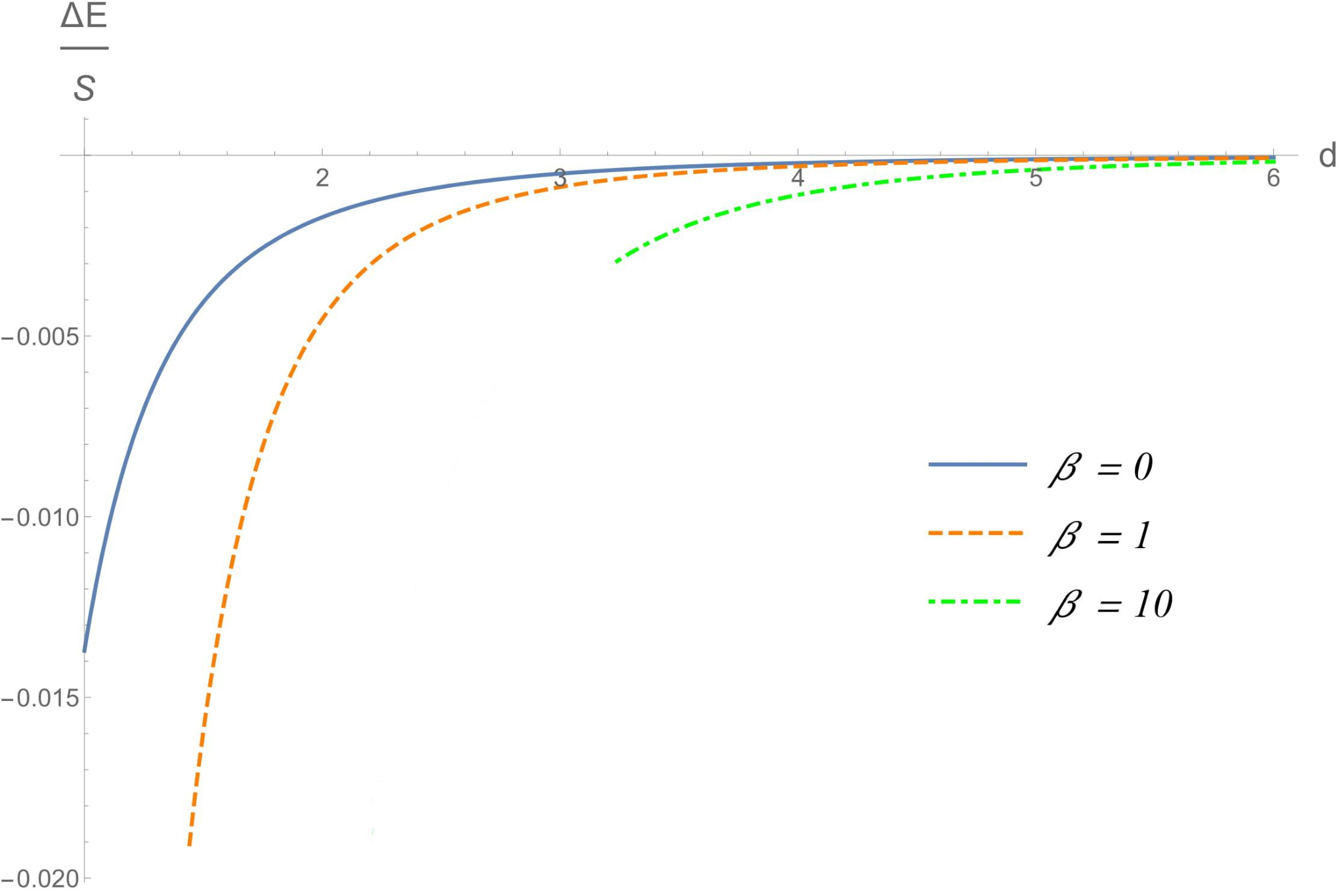
to be compared with the standard QED expression (7). Note that the GUP term is attractive, since it contributes to increase the modulus of the energy.

In Fig. 1, the Casimir energy per unit surface area has been plotted as a function of the distance between the plates for three values of the deformation parameter $\beta$. For distances large enough, the different curves overlap, being the effects of the minimal length negligible.

In Ref. Gine, the Casimir effect is derived from the idea that the contribution to the vacuum energy at a point $P_{0}$ of a plate is affected by the presence of the other boundary. Specifically, the author considers virtual photons produced by vacuum fluctuations somewhere in the space and arriving at $P_{0}$. In order to compute the total Casimir energy $\Delta E$, one has to take into account all the points on the surface $S$ of the plate. Therefore, from the HUP

($p=E/c$ for photons), the total contribution to the energy fluctuation $\Delta E$ is given by those photons in a volume $S\Delta x$ around the plate, where $\Delta x$ is the position uncertainty of the single particle. Note that, if we had only one plate, $\Delta x$ would be infinite, since photons may be created in any point of the space. However, this is no longer true in the presence of both the boundaries. In that case, indeed, virtual particles originating from behind the second plate cannot reach $P_{0}$. Thus, the additional plate acts as a sort of shield.

The above situation can be depicted as follows: consider a sphere of radius $R$ centered at the point $P_{0}$ and enclosing both the plates (see Fig. 2). In the single-plate configuration, the effective volume $S\Delta x$ corresponding to the entire space can be thought of as the total volume of the sphere $V_{T}=4/3\pi R^{3}$, with $R\rightarrow\infty$. Clearly, such a volume will be reduced by including the second plate, which will prevent particle that pop out in $P$ from impacting on $P_{0}$ (with reference to Fig. 2, the effective volume is represented by the shadowed region). As a result, we can write $S\Delta x=V_{T}-V_{C}$, where $V_{C}$ is the volume shielded by the second plate. In the case of infinite boundaries, or even better when $L/(2d)\rightarrow\infty$, one can show that $V_{C}=2/3\pi R^{3}$, yielding Gine

In the above treatment, no length scale has been considered, hence the volume $S\Delta x$ diverges as the radius $R$ increases. To cure such a pathological behavior, in Ref. Gine the author introduces a cutoff $r_{e}$ representing the effective distance beyond which photons have a negligible probability to reach the plate. In this way, Eq. (14) can be rewritten as

which has indeed a finite value. Combining this relation with the HUP, we then obtain

which implies

from comparison with the exact expression (7) for the Casimir energy. Strictly speaking, we would have

Although the above derivation is straightforward and very intuitive, the discussion on the physical origin of the length cutoff $r_{e}$ appears to be rather obscure in some points. Therefore, in order to clarify the meaning of Eq. (17), let us focus on the computation of the Casimir effect in a simplified one-dimensional system: similar reasonings can be readily extended to three dimensions.

From the Heisenberg uncertainty relation, it is well-known that large energy fluctuations live for very short time and, thus, hard virtual photons of energy $\Delta E$ can only travel short distances of order $\hslash c/\Delta E$. As a consequence, the further these particles are created from a plate, the more negligible their contribution to the energy around that plate will be. Let us apply these considerations to the apparatus in Fig. 3. It is easy to see that virtual photons popping out in the strip of width $d$ on the right side of the right plate do not contribute to the Casimir effect, since their pressure is balanced by those photons originating between the plates. By contrast, photons coming from a distance greater than $d$ in the right region do not experience any compensation, because their symmetric “partners” on the left side are screened by the first plate. The overall result is a net force acting on the right plate from right to left. Of course, this argument can be symmetrically applied to the left boundary and provides a qualitative explanation for the origin of the attractive Casimir force.

Now, consider a point at a distance $x_{0}>d$ from one of the plates, as in Fig. 3. Virtual photons originate from quantum fluctuations in a small region around that point. Such a region, however, cannot be smaller than the (reduced) Compton length of the electron, $\lambda_{C}=\hslash/(m_{e}c)$, otherwise the energy amplitude of the fluctuation would exceed the threshold $E\simeq m_{e}c^{2}$ for the production of electron-positron pairs. Besides, photons produced at $x_{0}$ can impact on the plate (and therefore contribute to the Casimir force) only if their energy $E$ is such that $0<E<E_{0}$, where $E_{0}=\hslash c/x_{0}$. Particles of higher energy $E>E_{0}$, indeed, would recombine before reaching the plate, since the distance they travel is $x=\hslash c/E<\hslash c/E_{0}=x_{0}$.

We can now assume that photons coming from $x_{0}$ originate from fluctuations of energy $E$ with a probability given by a Boltzmann-like factor $f(E)=e^{-E/(m_{e}c^{2})}$. Thus, the total linear energy density (i.e. the energy per unit length) arriving on the plate will be

where, since we are dealing with the electromagnetic field, we have introduced the natural threshold of the electron mass/energy $m_{e}c^{2}$. In terms of the distance $x_{0}$, the above integral becomes

Finally, in order to get the contribution to the Casimir energy from all the photons which impact on the plate, we integrate over all the points $x_{0}$ such that $d<x_{0}<\infty$, obtaining

The integrals in Eqs. (20) and (21) can be easily evaluated by observing that, for $x$ large enough, the Boltzmann factor $e^{-\hslash/(m_{e}cx)}$ becomes approximately of order unity. This yields

and, hence

which is in good agreement with the QFT prediction (8). Similarly, one can show that the generalization to three dimensions leads to a result consistent with Eq. (7).

The physical relevance of the above discussion becomes clearer if we observe that probability distributions like those in Eq. (19) or (20) allow us to naturally interpret the effective radius $r_{e}$ in Eq. (15) as the distance from the plate below which the vast majority of photons contribute to the large part of the Casimir energy. More rigorously, we can define $r_{e}>d$ as the distance within which photons carrying the fraction $\gamma$ $(0<\gamma<1)$ of the total Casimir energy are created. In other terms, we can write

from which

Thus, setting $r_{e}\simeq 2.6\hskip 1.42262ptd$ (as in Eq. (18)) amounts to consider a fraction $\gamma\simeq 0.62$ of the total energy responsible for the Casimir effect.

The above picture is quite rough, since it relies on the adoption of a Boltzmann-like distribution for the energy of quantum vacuum fluctuations. As a result, it underestimates the fraction of photons produced within the distance $r_{e}$ from the plate. Considerable improvements can be achieved by employing more realistic functions $f(E)$ in Eq. (19). For further details on this topic, see Refs. Few and therein.

Let us now extend the above arguments to the context of the GUP. As in the previous Subsection, we shall focus for simplicity on the one-dimensional case. The generalization to three dimensions proceeds in a very similar fashion.

We start from the modified uncertainty relation (1), here recast in the form

By solving with respect to $\Delta E$, we obtain

where the only solution to be considered is the one with negative sign, as it reduces to the standard result for vanishing $\beta$ (conversely, the solution with positive sign has no evident physical meaning). After expanding to the first order in $\beta$, it follows that

If we now neglect those photons coming from distances greater than the effective radius $r_{e}$, it is natural to assume the uncertainty position $\Delta x$ of the single photon to be of the order of $r_{e}$ and, thus, of $d$, according to Eq. (18). Then, by replacing $\Delta x\simeq 2.6\hskip 1.42262ptd$ into Eq. (28), the contribution to the Casimir energy at a given point reads

which indeed agrees with Eq. (8) in the limit $\beta\rightarrow 0$.

The above considerations can be now generalized to three-dimensions by taking into account the contribution to the zero-point energy at any point of the plates of area $S$. In doing so, straightforward calculations lead to

which is to be compared with Eq. (12). In spite of our skinny assumptions, one can see that the obtained expression agrees with the field theoretical result as concerns the dependence of the GUP correction on the inverse fifth power of the distance between the plates. We also notice that the exact numerical coefficient can be recovered by including a proper factor which accounts for the extension of the GUP (26) to a higher-dimensional system.

By following the same reasoning as for parallel plates, let us consider a spherical shell of (finite) radius $a$ enclosed in a larger sphere of (infinite) radius $R$ representing the whole space (see Fig. 4). By taking a point $P_{0}$ on the surface of the shell, one can easily understand that the only photons which are allowed to impact on $P_{0}$ are those originating from vacuum fluctuations in the shadowed volume. In light of this, we can write the effective volume $S\Delta x$ as the sum of the volume of the upper (external) hemisphere and the one of the shell, i.e.

where $S=4\pi a^{2}$ is the surface area of the shell. For the internal consistency of our formalism, we require $0<a\leq R/\sqrt[3]{2}$. By drawing a comparison with the parallel-plate system, the $a\rightarrow 0$ limit corresponds to the case in which the two plates are stuck together. In this case, the spherical shell degenerates into a single point, since $P_{0}$ merges with its antipode. Consequently, the effective volume $S\Delta x$ will be twice the volume of the hemisphere of radius $R\rightarrow\infty$, i.e. it will cover all the space²² 2 In order to compute the effective volume relative to $P_{0}$ for $a\rightarrow 0$, we must also take into account the symmetric contribution of those photons which impact on the antipode of $P_{0}$.. On the other hand, for $a=R/\sqrt[3]{2}\rightarrow\infty$, the point $P_{0}$ is not affected by the presence of the walls of the shell. This amounts to the case where the two parallel plates are infinitely far apart from each other. Again, the effective volume will be equal to the whole space, i.e. $S\Delta x=4\pi R^{3}/3\rightarrow\infty$ from Eq. (31).

Now, by using Eq. (31), the position uncertainty $\Delta x$ reads

that still diverges as $R$ increases. As for the parallel plates, however, we can reasonably neglect photons coming from distances greater than the effective radius $R\sim r_{e}$. By combining Eq. (32) with the HUP, it follows that

If we now assume $r_{e}$ to be of the order of the size of the system as in Eq. (18), i.e. $r_{e}\simeq 2.6\,(2\hskip 0.56905pta)$, we finally obtain

that matches with the QFT result of Refs. Boyer; Milton, up to a factor $1/2$ (as discussed after Eq. (25), one may improve the agreement by refining the considerations on the photon energy distribution as in Eq. (19)). Note that we cannot infer any kind of information on the sign of $\Delta E$, and, thus, on the nature of the Casimir force (whether it is attractive or repulsive), since our heuristic calculations only allow to derive the absolute value of the energy shift. In this regard, we emphasize that the issue of the sign of the zero-point force for a spherical shell is quite controversial. In Refs. Boyer; Milton, for instance, it is argued that a conducting sphere would tend to be expanded due to effects of vacuum fluctuations. On the other hand, if one roughly approximates the sphere as two parallel plates of area $S=\pi a^{2}$ and separation $d\simeq a$ and considers the standard expression (7) for the energy, the opposite sign for the Casimir force would be obtained³³ 3 Note that the idea to describe a sphere as two (circular) parallel plates was originally proposed by Casimir to calculate the fine-structure constant $\alpha$. Casimirsphere. A similar result is claimed to be valid for two slightly separated hemispheres (that is, a spherical shell sliced with a very subtle knife) and, more generally, for any symmetric configuration (see Kenneth-Klick’s no-go theorem KK).

Let us now investigate to what extent the zero-point Casimir energy (34) gets modified by the Generalized Uncertainty Principle (26). To this aim, by replacing Eq. (32) into (28), we get

where we have implicitly made use of the length cutoff $R\sim r_{e}$. By setting $r_{e}\simeq 2.6\hskip 1.42262pt(2\hskip 0.56905pta)$ as before, we find

Hence, on the basis of purely heuristic arguments, we obtain a GUP term scaling as the inverse cube of the radius of the spherical shell. As expected, the greater the sphere, the smaller the correction to the standard (HUP) result. Unlike the parallel-plate configuration, however, a full-fledged field theoretical calculation has not yet been carried out, thus preventing us from making any comparison.

We now compute the zero-point energy for a cylindrical shell of radius $a$ and height $H$. As depicted in Fig. 5, we assume $H>a$; however, similar considerations hold true for any size of the system.

Let us consider a point $P_{0}$ on the lateral surface of the cylinder. In this case, we can write the effective volume as

where now $S=2\pi\hskip 0.56905pta\hskip 0.56905ptH$ is the lateral surface of the cylinder and we have already implemented the cutoff $R\sim r_{e}$ on the radius of the surrounding sphere. Again, as $a$ and $H$ increase, the cylindrical shell tends to cover the whole space, while for vanishing $a$ and $H$, it collapses in a single point. In both cases, the effective volume will be equal to the entire space (see the discussion after Eq. (31)).

By inverting Eq. (37) with respect to the uncertainty position of photons, we get

which leads to the following expression of the standard (HUP) energy uncertainty:

Let us now observe that, since we are neglecting vacuum fluctuations from distances greater than $r_{e}$, it is reasonable to assume $H\simeq 2\hskip 0.85358ptr_{e}$ (in other terms, the only photons which can impact on $P_{0}$ moving from the inside to the outside of the cylinder are those in the volume $V\simeq\pi a^{2}\hskip 0.56905pt(2\hskip 0.56905ptr_{e})$). By setting $r_{e}\simeq 2.6\,(2\hskip 0.56905pta)$ as before, we then obtain

where we have computed the energy per unit length in order to compare our expression with the QFT result of Ref. DeRaad:1981hb. Note that the two outcomes are in good agreement with each other.

As usual, corrections induced by the GUP can be estimated by inserting Eq. (38) into Eq. (28). Straightforward calculations yield

which, for $r_{e}\simeq 2.6\hskip 1.42262pt(2\hskip 0.56905pta)$, becomes

As for the sphere, a QFT treatment of Casimir effect for a cylindrical shell is missing so far.

References

- (1) H. B. G. Casimir, Indag. Math. 10 (1948) 261 [Kon. Ned. Akad. Wetensch. Proc. 51 (1948) 793] [Front. Phys. 65 (1987) 342] [Kon. Ned. Akad. Wetensch. Proc. 100N3-4 (1997) 61].
- (2) K. A. Milton, The Casimir effect: Physical manifestations of zero-point energy, River Edge, USA: World Scientific (2001).
- (3) G. Benenti, A. D’Arrigo, S. Siccardi and G. Strini, Phys. Rev. A 90 (2014) 052313.
- (4) O. S. Andersen, R. E. A. Koeppe, Ann. Rev. Biophys. Biomol. Struct. 36 (2007) 107.
- (5) R. L. Jaffe, Phys. Rev. D 72 (2005) 021301.
- (6) M. Blasone, G. G. Luciano, L. Petruzziello and L. Smaldone, Phys. Lett. B 786 (2018) 278; A. Capolupo, I. De Martino, G. Lambiase and A. Stabile, Phys. Lett. B 790 (2019) 427.
- (7) K. Kikkawa and M. Yamasaki, Phys. Lett. 149B (1984) 357; S. D. Odintsov, Mod. Phys. Lett. A 3 (1988) 1391; F. Sorge, Class. Quant. Grav. 22 (2005) 5109; S. A. Fulling, K. A. Milton, P. Parashar, A. Romeo, K. V. Shajesh and J. Wagner, Phys. Rev. D 76 (2007) 025004.
- (8) M. Blasone, G. Lambiase, L. Petruzziello and A. Stabile, Eur. Phys. J. C 78 (2018) 976.
- (9) G. Lambiase, A. Stabile and A. Stabile, Phys. Rev. D 95 (2017) 084019; L. Buoninfante, G. Lambiase, L. Petruzziello and A. Stabile, Eur. Phys. J. C 79 (2019) 41.
- (10) K. Nouicer, J. Phys. A 38 (2005) 10027.
- (11) U. Harbach and S. Hossenfelder, Phys. Lett. B 632 (2006) 379.
- (12) O. Panella, Phys. Rev. D 76 (2007) 045012.
- (13) A. M. Frassino and O. Panella, Phys. Rev. D 85 (2012) 045030.
- (14) G. Carvalho Dorsch and J. A. Nogueira, Int. J. Mod. Phys. A 27 (2012) 1250113.
- (15) D. Amati, M. Ciafaloni and G. Veneziano, Phys. Lett. B 197 (1987) 81; D. J. Gross and P. F. Mende, Phys. Lett. B 197 (1987) 129; D. Amati, M. Ciafaloni and G. Veneziano, Phys. Lett. B 216 (1989) 41; K. Konishi, G. Paffuti and P. Provero, Phys. Lett. B 234 (1990) 276.
- (16) M. Maggiore, Phys. Lett. B 319 (1993) 83.
- (17) A. Kempf, G. Mangano and R. B. Mann, Phys. Rev. D 52 (1995) 1108.
- (18) F. Scardigli, Phys. Lett. B 452 (1999) 39.
- (19) R. J. Adler and D. I. Santiago, Mod. Phys. Lett. A 14 (1999) 1371; S. Capozziello, G. Lambiase and G. Scarpetta, Int. J. Theor. Phys. 39 (2000) 15.
- (20) A. Kempf and G. Mangano, Phys. Rev. D 55 (1997) 7909; F. Scardigli and R. Casadio, Class. Quant. Grav. 20 (2003) 3915.
- (21) R. Casadio, R. Garattini and F. Scardigli, Phys. Lett. B 679 (2009) 156.
- (22) R. Casadio and F. Scardigli, Eur. Phys. J. C 74 (2014) 2685.
- (23) F. Brau, J. Phys. A 32 (1999) 7691; D. Gao and M. Zhan, Phys. Rev. A 94 (2016) 013607; D. Gao, J. Wang and M. Zhan, Phys. Rev. A 95 (2017) 042106; Z. W. Feng, S. Z. Yang, H. L. Li and X. T. Zu, Phys. Lett. B 768 (2017) 81; P. Bosso, S. Das and R. B. Mann, Phys. Lett. B 785 (2018) 498.
- (24) F. Scardigli, G. Lambiase and E. Vagenas, Phys. Lett. B 767 (2017) 242; E. Vagenas, S. M. Alsaleh and A. Farag, EPL 120 (2017) 40001; T. Kanazawa, G. Lambiase, G. Vilasi and A. Yoshioka, Eur. Phys. J. C 79 (2019) 95; G. G. Luciano and L. Petruzziello, Eur. Phys. J. C 79 (2019) 283; L. Buoninfante, G. G. Luciano and L. Petruzziello, Eur. Phys. J. C 79 (2019) 663; J. Pye, J. Phys. Conf. Ser. 1275 (2019) 012025.
- (25) F. Scardigli, J. Phys. Conf. Ser. 1275 (2019) 012004.
- (26) R. J. Adler, P. Chen and D. I. Santiago, Gen. Rel. Grav. 33 (2001) 2101; G. Amelino-Camelia, M. Arzano, Y. Ling and G. Mandanici, Class. Quant. Grav. 23 (2006) 2585; M. Rizwan and K. Saifullah, Int. J. Mod. Phys. D 26 (2017) 1741018; Y. C. Ong, JCAP 1809 (2018) 015.
- (27) F. Scardigli, Nuovo Cim. B 110 (1995) 1029; F. Scardigli, M. Blasone, G. Luciano and R. Casadio, Eur. Phys. J. C 78 (2018) 728.
- (28) F. Scardigli, Proceedings (p.157-160), 18th Workshop on General Relativity and Gravitation in Japan (JGRG18), Hiroshima, Japan, November 17-21, 2008.
- (29) J. Giné, Mod. Phys. Lett. A 33 (2018) 1850140.
- (30) M. Bordag, G. L. Klimchitskaya, U. Mohideen and V. M. Mostepanenko, Int. Ser. Monogr. Phys. 145 (2009) 1.
- (31) C. J. Fewster, L. H. Ford and T. A. Roman, Phys. Rev. D 85 (2012) 125038; Springer Proc. Phys. 157 (2014) 489.
- (32) T. H. Boyer, Phys. Rev. 174 (1968) 1764.
- (33) C. M. Bender and K. A. Milton, Phys. Rev. D 50 (1994) 6547.
- (34) H. B. G. Casimir, Physica 19 (1953) 846.
- (35) O. Kenneth and I. Klich, Phys. Rev. Lett. 97 (2006) 160401.
- (36) L. L. DeRaad, Jr. and K. A. Milton, Annals Phys. 136 (1981) 229.
- (37) U. Mohideen and A. Roy, Phys. Rev. Lett. 81 (1998) 4549; G. Bressi, G. Carugno, R. Onofrio and G. Ruoso, Phys. Rev. Lett. 88 (2002) 041804.
- (38) J. Marino, A. Noto and R. Passante, Phys. Rev. Lett. 113 (2014) 020403; M. Blasone, G. Lambiase and G. G. Luciano, Phys. Rev. D 96 (2017) 025023; F. Dahia and P. J. F. da Silva, Class. Quant. Grav. 32 (2015) 177001; M. Blasone, G. Lambiase and G. G. Luciano, J. Phys. Conf. Ser. 880 (2017) 012043.
- (39) M. Blasone, P. Jizba and G. G. Luciano, Annals Phys. 397 (2018) 213; M. Blasone, G. Lambiase, G. G. Luciano and L. Petruzziello, Phys. Rev. D 97 (2018) 105008; B. Sokolov, J. Louko, S. Maniscalco and I. Vilja, arXiv:1806.07662 [quant-ph]; R. Carballo-Rubio, L. J. Garay, E. Martín-Martínez and J. De Ramón, Phys. Rev. Lett. 123 (2019) 04160; M. Blasone, G. Lambiase, G. G. Luciano and L. Petruzziello, Phys. Lett. B 800, 135083 (2020).
- (40) M. Blasone, G. Lambiase, G. G. Luciano and L. Petruzziello, EPL 124 (2018) 51001; F. Becattini, Phys. Rev. D 97 (2018) 085013; M. Blasone, G. Lambiase, G. G. Luciano and L. Petruzziello, J. Phys. Conf. Ser. 1226 (2019) 012027; A. G. S. Landulfo, S. A. Fulling and G. E. A. Matsas, Phys. Rev. D 100 (2019) 045020.