A Multilayered Block Network Model to Forecast Large Dynamic Transportation Graphs: an Application to US Air TransportJournal: Elsevier
Abstract
Dynamic transportation networks have been analyzed for years by means of static graph-based indicators in order to study the temporal evolution of relevant network components, and to reveal complex dependencies that would not be easily detected by a direct inspection of the data. This paper presents a state-of-the-art probabilistic latent network model to forecast multilayer dynamic graphs that are increasingly common in transportation and proposes a community-based extension to reduce the computational burden. Flexible time series analysis is obtained by modeling the probability of edges between vertices through latent Gaussian processes. The models and Bayesian inference are illustrated on a sample of 10-year data from four major airlines within the US air transportation system. Results show how the estimated latent parameters from the models are related to the airline’s connectivity dynamics, and their ability to project the multilayer graph into the future for out-of-sample full network forecasts, while stochastic blockmodeling allows for the identification of relevant communities. Reliable network predictions would allow policy-makers to better understand the dynamics of the transport system, and help in their planning on e.g. route development, or the deployment of new regulations.
Keywords:
transportation networks , multilayer graphs , air transport , machine learning1 Introduction and related work
We live in a highly interconnected world, and networks have become an integral part of our life, from telecommunications and social media to transportation systems and the Internet of Things. Further technological advances and the advent of automation, which may enable the autonomous operation of actors within the network, are likely to push the scale and sophistication of network systems up to new levels in the near future. This increasing complexity has permeated into science in a natural way, and the use of network modeling has become widespread in disciplines as diverse as Sociology, Neuroscience or Transportation [Jasny et al., 2009, Barabási, 2016], propelled by the availability of data and computing power. Transportation science has been for many decades an active field aiming for the development of models and policies that ensure the efficiency, safety and social acceptability of transportation systems, while limiting costs and environmental impact. In recent years there has been a growing number of research directions that reveal the need for appropriate methods to address the complexity imposed by network problems. Network resilience analysis against e.g. natural disasters or terrorist attacks, structural evolution of network systems, and network-wide traffic forecasting, are examples of these new directions. The interest in modeling and understanding transportation networks is not merely academic. The maritime shipping network processes over 80% of the world trade, whereas travel and tourism industries, which sustain 10% of the global GDP, rely on the air transport network (UNCTAD, 2017, WTTC, 2018). Also, public transport networks are a key element in the infrastructure of large urban areas, where the bulk of the economic activity is concentrated in most developed countries.
Here we focus on multilayer dynamic networks and use latent variable models for analyzing complex graph data that are increasingly available in transportation and related fields. Multilayer networks add a new dimension to the network representation through the definition of layers, and allow for the modeling of complex systems that would be difficult to represent using regular, "flat" graphs. Multilayer networks can be defined and structured in various ways depending on the problem and the specific role of the layers [Kivelä et al., 2014]. In transportation, a multilayer graph could represent how different airlines interact with the underlying airport network, or how different transport modes (e.g. bus and metro networks) operate simultaneously within a public transportation system. Dynamic networks, on the other hand, add a temporal dimension to the problem by assuming that the interaction between the elements in the network change over time, which is common in transport systems, as discussed below. A latent network model [Kolaczyk, 2017, Crane, 2018] is a probabilistic model that uses unobserved features to characterize different properties and processes within a graph. These models are flexible and allow for e.g. link prediction and community detection, and are also relatively easy to estimate, see Section 2 for further details and relevant literature.
Dynamic transportation networks have been studied for years, both from short-term and long-term perspectives. Studies featuring a long-term approach usually aim to analyze the structural dynamics of the transportation system in order to assess the temporal evolution of relevant network components in terms of months or years, and to reveal complex dependencies and patterns that would not be easily detected by a direct inspection of the data. A graph-based analysis through the use of measures such as e.g. the node degree or betweenness (Guimera et al., 2005) became the de facto methodological approach, which has been also used to study the dynamics of shipping and airport networks [Ducruet and Notteboom, 2012, Wang et al., 2014], or airline de-hubbing [Rodríguez-Déniz et al., 2013], among many others. On the other hand, short-term network dynamic problems usually deal with time spans of minutes or hours, and focus on modeling specific elements within the network (e.g. link congestion) rather than adopting a structural approach. A good example of a short-term network problem in transportation is urban traffic forecasting. This is a time-series prediction problem that has been traditionally addressed with statistical and machine learning models [Vlahogianni et al., 2014], and where a explicit graph-based representation of the network is not strictly necessary. We believe there is an opportunity for a methodological advance in studies involving the long-term analysis of transportation networks by using state-of-the-art statistical models for dynamic and multilayer graph data, therefore moving from the current descriptive, indicator-based approach to an inferential one. Moreover, reliable graph forecasting would allow for the definition of benchmarking scenarios in problems where origin-destination pairs are usually assumed fixed. Examples of those applications would be airline schedule optimization [Cadarso and de Celis, 2017], cargo assignment in shipping networks [Wang et al., 2016] and hub-location [Alkaabneh et al., 2019], to name a few.
In spite of the above, there have been some recent contributions to model-based inference in transportation graphs. A representative example is the paper from Kotegawa et al., 2010, which addresses the problem of route (link) prediction in air transportation networks. Their work is motivated by the air traffic forecasts from the US Federal Aviation Administration (FAA), which does not consider network dynamics in their predictions. The authors tackle the graph forecasting problem by training a model that uses topological characteristics of the airports as covariates, and yield the probability of city-pairs being connected by new routes in the future. Three competing models (logistics regression, neural networks, and a preferential attachment algorithm) were tested, with the artificial neural network being the top performer. The authors stress that given the competitive nature of the airline industry and its implications on the network’s structure (e.g. dehubbing), reliable network forecasts would allow policy-makers to better understand the dynamics of the system, and help in their planning on e.g. infrastructure development, or the deployment of new regulations. Similarly, de Wit and Zuidberg, 2016 perform an econometric analysis to study the probability of market closures for European low-cost carriers. They implement a logistic regression model with route-based covariates (e.g. distance, offered seats) that could help identify the factors that make markets more likely to be canceled, although their approach lack the network and dynamic perspective.
Working with large graphs can be computationally tough, and transportation networks are no exception to that. A practical way to circumvent this issue that has been recently adopted in the literature is to reduce the scale of the problem by partitioning the graph. In graph clustering, also known as community detection (see e.g. Fortunato, 2010) or stochastic blockmodeling (Nowicki and Snijders, 2001, Airoldi et al., 2008), the objective is to find groups of highly interconnected elements within the network, which may reveal structures such as e.g. social cliques or spatial patterns. In a public transport context, Yap et al., 2019 used a two-pronged strategy to reduce the size of their transfer synchronization problem. First they performed spatial clustering to isolate relevant transfer locations, and then used graph-based community detection to determine which line bundles within the selected hubs to synchronize. Tian et al., 2020 greatly reduced the computational cost in a large-scale rebalancing problem by clustering their bike-sharing network into five management areas. Still, graph clustering has not been exclusively used to deal with the computational bottleneck. Yildirimoglu and Kim, 2018 use modularity-based community detection to find demand patterns in an urban multilayer setting (bus, passenger and car networks), thus allowing for a demand analysis at different spatial resolutions that may be helpful for planning and operation, whereas Olmos et al., 2020 identified relevant demand clusters for a better design of a network of bicycle paths. One aspect that is common among the previous studies is that the clustering is framed as a separate spatial problem, without explicitly considering the dynamics of the network.
The aim of this paper is threefold: i) present a state-of-the-art latent network model to forecast multilayer dynamic graphs that are increasingly common in transportation, which have potential applications to the long-term analysis of transportation networks, ii) propose a community-based extension of the model to reduce the computational burden by jointly considering the temporal and spatial dimensions of the network, and iii) demonstrate their applicability to a real multilayer transportation network in two case studies with US airline data.
The rest of the manuscript is organized as follows. Section 2 briefly introduce relevant work on statistical models for network data. The methodological framework and the community-based model are detailed in Section 3, whereas in Section 4 a set of validation experiments are performed. Section 5 presents applications to real data from an airline network. The last section summarizes the paper and discuss limitations and possible directions for further research.
2 Statistical models for graph data
Statistical network analysis is a well-established field of research (see e.g. Kolaczyk, 2009) with origins dating back to the seminal work on random graphs by Erdös and Renyi, 1959. Despite their fundamental contributions, the original mathematical models, along with other recent models such as the “small-worlds” from Watts and Strogatz, 1998 and the hub-and-spoke networks from Barabási and Albert, 1999, are too limited for most applications. Exponential Random Graph Models (ERGMs) were designed with this aim in mind, initially with the model from Holland and Leinhardt, 1981, and define an exponential family of distributions over a graph. However, model degeneracy and intractability are still unresolved problems, which has represented a hurdle for a wider applicability outside social networks. Interestingly, Zhang et al., 2019 recently used ERGM models to learn social networks effects that can be used to generate synthetic populations in agent-based transport simulators.
In contrast with the log-linear approach of the ERGMs, latent network models (LNMs) define latent classes or features to capture the network complexity in a non-linear fashion. The Stochastic Block Model (SBM - Holland et al., 1983) is perhaps the most popular latent network model, and assumes a latent community structure that drives the relationship patterns between actors in the network. Nowicki and Snijders, 2001 proposed a Bayesian inference algorithm using Gibbs sampling whereas Daudin et al., 2008 developed variational inference for the model. Current research on SBM’s is mainly aimed at mixed membership clustering (Airoldi et al., 2008), extensions for weighted graphs (Aicher et al., 2014), dynamic and state-space modeling (Ishiguro et al., 2010, Xu and Hero, 2014), and multi-layer networks (Han et al., 2015, Stanley et al., 2016). A different approach to LNMs is to define a latent space over the network nodes themselves (Hoff et al., 2002). In this case, the probability that two network elements are connected can be defined in terms of a distance function, in such a way that nodes neighboring in the unobserved latent space are more likely to be connected. Latent space models are able to capture transitive dependencies in a natural way (in contrast with SBM’s) and are flexible enough to incorporate dynamics while allowing for practical maximum likelihood and Bayesian inference. More recently, Durante and Dunson, 2014 introduce exact Bayesian inference using Pólya-Gamma augmentation (Polson et al., 2013) for a dynamic latent space network model driven by Gaussian Processes. A natural extension of the previous model to a dynamic multilayer setting is presented in Durante et al., 2017, although scalability issues arise for large network data since the model introduces a Gaussian process for each node in each layer.
3 Methodology
3.1 Dynamic Multilayered Network Model
We first describe the dynamic multilayered network model in Durante and Dunson, 2014 and Durante et al., 2017 that serves as a starting point for our community-based extension. We represent a network as a graph where is the set of vertices (also called nodes) and a set of unweighted edges (also called links) between node pairs . The connectivity of the graph is summarized in the adjacency matrix , where if there is an edge connecting vertices and , and otherwise. We assume undirected edges and no self-loops, i.e. and . Dynamic multilayer graphs have a graph per layer that evolves in time and can be represented by adjacency matrices where if vertices and are connected in layer at time .
The dynamic multilayer network model in Durante and Dunson, 2014 and Durante et al., 2017 defines a Bayesian logistic regression for each element in the adjacency matrix , i.e. for each possible edge in the graph at any layer and time . The logit of the probability that any two vertices in the multilayer graph are connected depends on a model with three additive components featuring unobserved variables that encode connectivity patterns. Specifically, the model is of the form
| (1) |
where the latent processes, , and , are assumed to be smoothly evolving Gaussian processes with RBF kernel functions (Rasmussen and Williams, 2006)
| (2a) | ||||
| (2b) | ||||
| (2c) | ||||
The model is structured through a set of latent variables that capture different effects within the network. The global time-varying intercept defines a baseline network density for all nodes in all layers. The cross-layer effects enter as a bilinear form [Hoff, 2005], increasing the probability of a link between vertices as their latent coordinates become aligned whereas the within-layer coordinates act in an identical manner capturing those effects not shared across the different layers. Instead of learning the dimensionality and of the latent coordinates and , the model uses multiplicative inverse Gamma priors [Bhattacharya and Dunson, 2011] to induce a shrinkage effect that becomes stronger for larger and
| (3) |
| (4) |
| (5) |
| (6) |
Durante et al., 2017 prove that the model in Eq.(1) is very flexible and can essentially model any matrix of edge probabilities if and is large enough. The likelihood factorizes into a set of Bernoulli logistic regressions which can be Gibbs sampled using the Pólya-Gamma data augmentation in Polson et al., 2013. However, the number of Gaussian processes that needs to be learned from data is , which makes computations and storage unmanageable for anything except small networks with few layers and small number of nodes. Moreover, the model is completely unstructured and is therefore massively overparametrized when the data follow some structure, e.g. some sort of community clustering. In the next section we propose a SBM extension of the model with a dramatically reduced number of Gaussian processes and develop a Gibbs sampling algorithm for inference using the Pólya-Gamma data augmentation trick. The model imposes a community structure and is therefore less general than Durante et al., 2017, but benefits from a reduction in the number of Gaussian processes and scales much better to larger networks.
3.2 Dynamic Multilayered Block Network Model
To impose a community structure we assume that each vertex in the network belongs to a stochastic block (Nowicki and Snijders, 2001) or cluster with prior probability , where is the vector of block assignments, indicating to which block each vertex belongs, and . This results in logistic regressions that model the interactions between groups of vertices, i.e. the probability of the existence of an edge between any two vertices in the network now depends on which block/cluster they belong. We propose the following block model extension of Durante et al., 2017
| (7) | ||||
| (8) |
The link probabilities for are of the same form as in Durante et al., 2017, but here defined over blocks, for a given block assignment. The within-block link probabilities for are modeled separately with a dynamic intercept per block and layer , and a second term with the sum of cross-layer coordinates of the corresponding block that allows for some block-wise leveraging between the two logits. See Figure 1 for a graphical representation.
3.3 A Scalable Gibbs Sampler for Bayesian Inference
The complete-data likelihood for the proposed model is
where , and and are the number of possible and actual edges in between blocks and , respectively. The block model induces a set of within-block summations over edges that structures the likelihood into explicit Binomial components instead of the Bernoulli components in Durante et al., 2017. This likelihood allows for exact Bayesian inference using Gibbs sampling with the Pólya-Gamma data augmentation for Binomial logistic regression in Polson et al., 2013, while automatically reducing the model size for large network problems as the estimation will be over blocks instead of vertices, where .
In B.1 we briefly review the Pólya-Gamma data augmentation method (Polson et al., 2013), which provides a tractable, efficient way to perform Bayesian inference on models with binomial likelihoods, whereas B.2 gives a detailed description of a Gibbs sampler algorithm to sample from the joint posterior of all model parameters. The sampler combines the multilayer network model from Durante et al., 2017, modified to our specific structure of the block link probabilities in Eq.(8), with updating steps for the latent block allocations and block probabilities following Nowicki and Snijders, 2001.
The Gibbs sampler in Durante et al., 2017 involves draws from the distribution. B.2 shows that this step in our algorithm includes updating step for the Pólya-Gamma variables , where . Hence, although the number of draws is dramatically smaller for our algorithm, each draw tends to be more costly since the time to simulate from increase in . To speed up computations we follow up on the suggestion mentioned in Windle et al., 2014 and develop a fast normal approximation via moment-matching; see A. Figure 2 (left) show the mean absolute error between the normal approximation and the sampling methods from [Devroye, 2009, Polson et al., 2013], relative to the theoretical mean. We see that for values of the deviation from the theoretical mean is less than 20% in the worst case where and negligible for . Simulation times are independent from when sampling from the approximation (right). Therefore, we use our normal approximation to sample Pólya-Gamma variables for , and the standard exact methods otherwise.
The update of the block assignments in the last step of the Gibbs sampler implies the computation of the posterior of the latent assignment probabilities for each node in the network (see step 10 in B.2). A naïve implementation will result in time, which could be prohibitive for large , specially if we update all sequentially at each MCMC iteration. We recommend an annealed random-scan sampling that starts updating the entire network and exponentially decreases the number of vertices being updated to a small fraction as the estimation progress. This would allow the Gibbs sampler to initially explore a large space of possible clusterings at a higher computational cost, and then concentrate the estimation effort on the parameters defining the block dynamics while still allowing for some refinement in the assignments.
4 Simulation study
In this section we use synthetic data to compare the fitting capability and estimation time of the DMN model in Durante et al., 2017 with our DMBN model with block structure. We simulate multilayer networks with sizes ranging from and different levels of granularity: . We also simulate networks from the DMN model without block structure. All networks have the same number of layers and time points, and are generated from a dynamic six-dimensional latent space, i.e. , with common smoothness over all components. Each latent coordinate are simulated from three predefined types of connectivity patterns: i) smoothed constant, ii) smoothed seasonal connectivity and iii) smoothed linear trend. Table 1 shows the parameter configuration that is used by both models during the simulations, which were performed on a cluster from the Swedish National Supercomputer Center (NSC-SNIC).
| Model | MCMC Samples | |||||||||
|---|---|---|---|---|---|---|---|---|---|---|
| DMN | - | 6 | 6 | 0.05 | - | 0.05 | 0.05 | 2 | 2 | 5,000 (20% burnin) |
| DMBN | 10 | 6 | 6 | 0.05 | 0.05 | 0.05 | 0.05 | 2 | 2 | 5,000 (20% burnin) |
| (a) | (b) | (c) | (d) No blocks | |
|---|---|---|---|---|
|
True |
||||
|
Estimated |
We estimated the models specified above to every simulated networks ten times with random initialization of block assignments and latent coordinates. Estimation times and performance metrics were averaged accordingly. Relative mean absolute errors (MAE) for estimating the true link probabilities are presented in Table 2. The results illustrate how the DMBN model takes advantage of the community structures to recover the link probabilities, effect that is more pronounced as the network size increases. For larger networks () and clear block structure () the DMBN model outperforms the DMN with relative MAE ratios of 3.65 and 4.20 respectively. On the other hand, the performance of the DMBN model decreases with granularity regardless of the network size. Absolute MAE’s for both models are between 0.01 and 0.08. Note that for the DMN model the number of latent coordinates grows rapidly with , and for networks of size the estimation times exceeded the limit from the computing infrastructure, thus relative measures are not shown. The fact that the block-based model is not able to fully recover all individual link probabilities at full granularity is an expected outcome since this model tries to summarize the dynamic of groups of links using a very limited set of parameters. As the granularity increases towards the worst-case-scenario of a multilayer network where the dynamics of each link is generated by its own stochastic process and the block structure vanishes, the DMBN is expected to be less effective to fit the data and outperformed by the DMN.
Figure 3 shows the true and estimated probabilities from the DMBN on four dynamic multilayer networks with nodes and different block structure. For each network (, and no block structure) the figure shows the probabilities from a randomly selected graph out of the entire set of graphs. The four images in the top row show the true probabilities, which appear clearly structured in (a-c) compared to the full-granularity graph in (d). In the bottom row we see how the DMBN is able to almost perfectly recover all probabilities when and , is doing a decent job when and, as expected, struggles to fit the DMN model without any block structure.
Table 3 presents the relative running times (originally in minutes) for all simulations. As expected, the capacity of the DMN model to capture network link dynamics at full granularity comes at the cost of time. The estimation of the DMN model is significantly slower compared to the DMBN, with running times ranging from twice () to more than thirty times slower to those from the DMBN for the network with nodes. For the DMBN the absolute estimation times are below one hour in most cases, and only grow noticeably when the network size is above , hence demonstrating the scalability of the model when . This assumption may hold true for many real networks, such as social or transportation networks, where community structure naturally arises. In the next section we present a case study using real data, and evaluate the classification performance of the proposed model to predict markets within the US airport system, a classic example of a hub-and-spoke network.
| Network Size | |||||
|---|---|---|---|---|---|
| True | 32 | 64 | 128 | 256 | 512 |
| 5 | 1.49 | 2.30 | 3.65 | 4.20 | - |
| 15 | 0.92 | 1.05 | 1.25 | 1.12 | - |
| 45 | 0.93 | 0.94 | 0.87 | 0.79 | - |
| No blocks | 1.13 | 1.11 | 0.92 | 0.73 | - |
| Network Size | |||||
|---|---|---|---|---|---|
| True | 32 | 64 | 128 | 256 | 512 |
| 5 | 2.15 | 5.93 | 16.80 | 31.52 | - |
| 15 | 2.19 | 5.86 | 16.38 | 32.07 | - |
| 45 | 2.14 | 5.76 | 16.32 | 32.12 | - |
| No blocks | 2.11 | 5.57 | 16.24 | 31.16 | - |
5 Application to the US air transport network
Modeling complex transportation systems as dynamic multilayer graphs [Kivelä et al., 2014] has been recently attempted for e.g. air transportation [Cardillo et al., 2013], public transport [Gallotti and Barthelemy, 2015] or maritime networks [Ducruet, 2017]. The majority of these contributions focus on the visual inspection of the graphs, or the temporal and multilayer analysis of the networks by means of static, layer-wise topological measures, with no use of statistical or machine learning models. In this case study we apply the model from Durante et al., 2017 and our community-based extension introduced in Section 3 to a real airline network with airports as nodes and airlines as layers. The dynamic and multilayer dimensions of the network are modeled jointly in a probabilistic fashion, and the stochastic block structure allows for interesting model-based clustering of airports. The data description is presented first, followed by two different study scenarios. In the first scenario we fit the DMN model to a small subnetwork of two airlines: Delta and Southwest. The objective is to investigate how the model estimates reflect changes in network structure due to the merger of Southwest and AirTran after 2011, and other events happened during the sample period. The second study features a full-scale forecasting application to a dynamic multilayer transport network with 80 airports and four airlines over a 10-year period. We compare both models in terms of classification performance and estimation times, and also investigate the resulting airport clusters from the DMBN. Table 5 summarizes the experimental setup and network data utilized in each case study. All experiments were implemented using R Open 3.4.2 (MKL support), and executed on an Intel i7 Dual-Core PC with 16 GB of RAM running Windows 10.
5.1 Data source and network description
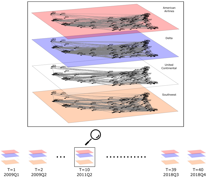
We collected publically available airline ticket data from the Airline Origin and Destination Survey (BTS, 2019a), from which we create the air transportation graphs. Figure 4 shows the mainland US airports available from the survey along with their hub classification [FAA, 2019]; we selected the airports with the largest number of (departing) flights, over a period of ten years (2009-2018). These airports concentrate around 95% of the total network traffic. The survey provides quarterly data so the number of time steps will be . To create a multilayer network, we generate separate graphs corresponding to major airlines: American Airlines, Delta, United/Continental and Southwest. Our choice of airlines is not random: after the mergers of Delta/Northwest (2009), United/Continental (2010), Southwest/AirTran (2011) and American Airlines/US Airways (2013), the resulting "big four" became the dominant airlines in the system. A graphical representation of the multilayer structure at the second quarter of 2011 is presented in Figure 5, and relevant network statistics in Table 4. We generated the multilayer graph using the library Pymnet [Kivelä, 2015]. All indicators but the number of flights are based on the corresponding unweighted, undirected graphs. We see similar network characteristics among the full-service carriers, whereas Southwest stands out with a higher edge density and less centralized degree distribution, which agrees with the tendency of low-cost airlines to relax the hub-and-spoke model by developing a significant number of point-to-point markets Doganis, 2019. Note also that there is only around 25% percent of edge-overlap between the different airlines, which justifies the use multilayer models.
| Layer | Nodes | Edges | Density | ASPL | Degree | Flights |
|---|---|---|---|---|---|---|
| 1 - AA | 80 | 579 | 0.092 | 1.948 | 14.486 | 206,078 |
| 2 - DL | 80 | 563 | 0.089 | 1.957 | 14.070 | 170,825 |
| 3 - UA | 80 | 557 | 0.088 | 1.975 | 13.912 | 125,464 |
| 4 - WN | 80 | 1,047 | 0.166 | 1.803 | 26.163 | 284,437 |
| Combined | 80 | 2,190 | 0.346 | 1.669 | 54.756 | 789,163 |
| Description | Selected graphs by quarter and year | ||||||||||
|---|---|---|---|---|---|---|---|---|---|---|---|
| Case study 1: model analysis | 09 | 10 | 11 | 12 | 13 | 14 | 15 | 16 | 17 | 18 | |
| Only DMN model | Q1 | ||||||||||
| Only Delta/Southwest (K=2) | Q2 | ||||||||||
| Subnetwork of N=40 airports | Q3 | ||||||||||
| Q4 | |||||||||||
| Case study 2: forecasting | 09 | 10 | 11 | 12 | 13 | 14 | 15 | 16 | 17 | 18 | |
| Both DMN/DMBN models | Q1 | ||||||||||
| All airlines (K=4) | Q2 | ||||||||||
| All airports (N=80) | Q3 | ||||||||||
| Q4 | |||||||||||
5.2 Merger of Southwest and AirTran (2011)
When Southwest acquired AirTran in 2011, it was the first merger between low-cost carriers in US history. Prior to the merge, Southwest carried almost 90 million passengers in 2010, more than triple than AirTran, and operated point-to-point markets, in contrast to the hub-and-spoke structure of AirTran’s network. The operation was appealing for Southwest, which not only had the opportunity to take over the network of its competitor, but also to enter Atlanta, which was at the time the only major US city without a strong presence of Southwest. This would help Southwest solidify its position as a dominant domestic low-cost carrier while adding some new international routes, mainly in the Caribbean, to its network. In this study, we investigate changes in the network graphs of Southwest and Delta, the dominant airline at Atlanta, as a consequence of the merger, and other potential causes between 2009-2018, using the dynamic multilayer model of Durante et al., 2017.
To that end, we fit the DMN model to a selected subset of the full multilayer graph shown in Figure 5, featuring airports from Delta and Southwest () networks, and keeping only the first quarter of every year (), see Table 5. Note that even though we will estimate logits, this scenario is rather conservative compared to the half-million required for the full problem, hence the need for the community-based extension. We draw posterior samples using similar hyperparameter values as for the simulations in Section 4, i.e. , with common smoothness over all components. Due to the bilinear forms in Eq. (1) the latent coordinates and are not identified and their estimates should not be interpreted directly. We follow Hoff, 2005 and calculate the posterior means of for each instead, which are identified, and then obtain estimators by truncating the spectral decompositions at the -th largest eigenvalue. The within-layer coordinates are recovered using the same procedure, for every layer and time point. Since the estimated coordinates contain information about the connectivity profile of every airport , it is straightforward to define cross and within layer vertex connectivity scores (VCS) as the euclidean norm of the coordinates, i.e.
| (9a) | |||
| (9b) | |||
Figure 6 present both scores for all airports in the sample as a function of the number of connections (i.e. degree). There seems to be a strong linear correlation between the within-layer scores and the degree of an airport, which is not present in the cross-layer estimates. This is probably related to our choice of mixing a legacy (hub-and-spoke) and a low-cost (point-to-point) carrier in the experiment. If airlines are significantly different in their structure and routes, their connectivity patterns will be absorbed by the layer effects, and the interpretation of the cross-layer connectivity scores may not be possible by direct inspection. We compared the scores against more elaborated centrality indicators such as betweenness and closeness, with similar results. The fact that the latent coordinates, which can be projected to future time steps, are related to topological properties from the underlying graph that determine the efficiency of air transportation in terms of e.g. passenger-kilometers Kotegawa et al., 2014, is an interesting outcome from the model.
In Figure 7 (left) we look directly at the two largest components from the estimated cross-layer coordinates for all airports in 2009. Even though there is no apparent clustering structure, there exists a general pattern based on airline dominance at the airports, and the fact that we left American Airlines and Continental out of the experiment. Airports that are close to the origin are mostly American (e.g. Miami, Dallas Fort-Worth), US Airways (e.g. Philadelphia) or United/Continental (e.g. Houston, Chicago O’Hare) hubs, whereas the most outlying airports are hubs for Delta (e.g. Atlanta, Salt Lake City) or focus cities for Southwest (e.g. Midway), with the exception of Los Angeles and Boston. In this case, a visual inspection of the coordinates for a specific year and quarter is sufficient, but a proper cluster analysis would probably be the best choice for their interpretation over time. Back to the vertex scores, Figure 7 (right) presents the dynamic evolution of the cross-layer and within-layer VCS for Atlanta-Hartsfield. We see how the within-layer score for Southwest grows steadily after the merger with AirTran in 2011 and the subsequent expansion at Atlanta. As a consequence, the cross-layer score is pushed up as both airlines hold now an important presence in that vertex, while the score for Delta decreases slightly though remaining high. Similarly, once the cross-layer score is significantly increased, Southwest’s score starts to diminish as well, which could be an indication on how the model tries to leverage the different components of the logit during estimation.
| Rank | CL-2009 | CL-2018 | DL-2009 | DL-2018 | SW-2009 | SW-2018 |
|---|---|---|---|---|---|---|
| 1 | SLC | ATL | ATL | ATL | MDW | MDW |
| 2 | LAX | LAX | SLC | SLC | DEN | DAL |
| 3 | DAL | LGA | JFK | MSP | LAS | DEN |
| 4 | OAK | MSP | LGA | DTW | PHX | STL |
| 5 | LGA | SLC | DTW | JFK | HOU | PHX |
| 6 | MSY | MCO | MSP | LAX | AUS | BNA |
| 7 | BWI | DAL | BOS | LGA | MCI | LAS |
| 8 | JFK | LAS | LAX | SEA | BWI | AUS |
| 9 | DTW | BWI | MCO | BOS | STL | HOU |
| 10 | LAS | OAK | TPA | LAS | BNA | BWI |
Table 6 presents airport rankings according to estimated vertex connectivity indices for the sample period. Overall, we get the expected actors at the top of the ranks, particularly at the airline (layer) level: Atlanta, Salt Lake City and Minneapolis lead Delta’s network, whereas Chicago Midway, Denver, Las Vegas and Dallas-Love are the top performers for Southwest. In the cross-layer rankings, we notice the rising of Minneapolis and Atlanta between 2009-2018, which is probably due to their acquisition by Delta and Southwest after the mergers with Northwest (2008) and AirTran (2011), respectively. In 2014, Delta increased its presence at Seattle airport in order to open a transoceanic hub, therefore entering into direct competition in the domestic market with Alaska Airlines at their major base. This is reflected on Delta’s within layer rankings with Seattle climbing from the -th to the -th position. From the Southwest’s perspective, Dallas Love-Field appears as the airport with largest increase in within-layer connectivity. This is an expected result: after the repealing of 1979’s Wright Amendment, which prohibited flights from Dallas Love-Field outside Texas and its neighboring states in order to protect Dallas Fort-Worth, Southwest greatly expanded at the former with 15 new routes in late 2014 CAPA, 2015. In Figure 8 (top row) we illustrate the model’s ability to capture the network’s dynamics during this expansion of Southwest at Love-Field, focusing on the new routes to/from Washington-Reagan, Portland and Tampa. Note how the underlying Gaussian processes that drive the logits adjust rapidly to changes in the network in all cases. Here the model’s flexibility in latent space has clearly paid off, despite the lack of exogenous (e.g. passenger traffic) information outside the adjacency matrices. We have experimentally verified that the estimated link probabilities are not sensitive to reasonable changes in the degree of shrinkage of the latent coordinates (as controlled by the hyperparameters in the Gamma prior), which control the effective dimensionality of the latent space. Similarly, the estimates are also robust to variation in the size of the latent coordinates , and the prior smoothness of the corresponding Gaussian processes. It is important to remark that the flexibility in latent space is due not only to the magnitude (e.g. connectivity scores) but also to the alignment (i.e. angles) of the vectors. For instance, the estimated cross-layer components can be written as , where the angles between the latent airport coordinates are a function of time. We finally corroborate this for our example in Figure 8 (bottom row): the cross-layer and layer-wise (Southwest) latent components of the new markets (2009-2018) are closer in angle to those of Dallas Love-Field.
5.3 Dynamic multilayer forecasting of the US air transport network
Despite its effectiveness, as we have just confirmed, fitting the original DMN model to very large graphs is not practical due to the over-parametrization and subsequent high estimation times. Here we test our proposed model extension by fitting and forecasting a large dynamic multilayer graph using all available airline data. The complete network features airports, airlines and time steps corresponding to quarters between 2009-2018. We compare both models in terms of classification accuracy and estimation times, and also investigate whether the block-wise structure of the DMBN model is able to reveal meaningful airport communities.
First we compare the performance of the DMN with the DMBN model. For both models we choose a , and a very smooth progression over time . We use the first nine years of the sample (36 quarters) for training the model, i.e. , and the last year for out-of-sample testing. Both models were run for 5,000 MCMC iterations and 20% burn-in, with a random-scan for the DMBN. Computing the posterior predictive distribution for the edge probabilities in the test sample is straightforward within the current Gibbs sampling framework, see Step 11 in B.2. Figure 9 (top-left) shows the ROC curves over the test data for the DMBN with blocks and the DMN. The DMN turns out to be a very accurate classifier, but is computationally very costly as it estimates logits, in contrast to the from the DMBN with blocks. The performance of the DMBN model increases with and takes substantially less time to estimate; estimation times (Figure 9, top-right) for the DMBN range from 25 minutes () to 1.5 hours (), and are at least one order of magnitude faster than the DMN, which needs almost 19 hours to be estimated. The layer-wise ROC curves presented below for the DMBN with blocks (left), and the DMN (right) also show how the least structured airline network (Southwest) is the most difficult to predict.
Figure 10 presents some adjacency matrices from the multilayer network,
and their estimated edge probabilities calculated from the posterior
samples of the DMBN model with blocks. All matrices are
in size, and their rows are ordered according to the airport’s IATA
codes (see D). Most adjacency matrices (top row) present
a clear hub-and-spoke layout, with few dominant airports connected
to all other nodes at a given layer, which is captured well by the
model through the estimated probabilities (bottom row). Note that
probability matrices in Figure 10 (bottom row) are not ordered according
to blocks but to airport codes, thus the block structure resulting
from the DMBN model is not clearly visible. The first column shows
the network of American Airlines at the last quarter of 2009, from
which we see how the model learned the connectivity patterns from
the adjacency matrix, assigning the highest probabilities to edges
connected to Charlotte, Dallas Fort-Worth, Miami, Chicago O’Hare and
Philadelphia. Having the latent block coordinates
entering as a bilinear form [Hoff, 2005] is convenient
here to capture the cross-like patterns exhibited by these hubs, as
airports with larger magnitudes in their latent space will increase
their connectivity with respect to every other node in the network,
regardless of the block they belong to. The estimated edge probabilities
for Delta in the third quarter of 2009 (second column) seem to have
captured the most relevant patterns, corresponding to the connections
of Delta’s major hubs, i.e. Atlanta, Detroit, Los Angeles, La Guardia,
Minneapolis and Salt Lake City. Similar results are obtained for United/Continental
in 2015 (third column) with Newark, Dulles, Houston International
and San Francisco, although some more noise is appreciated in the
estimated probabilities. The last column of Figure 10 shows the one-quarter-ahead
predicted edge probabilities in the test set for American Airlines.
| 2009Q4 - AA | 2012Q3 - DL | 2015Q2 - UA | 2018Q1 - AA |
Airline densities and airport degrees can be readily calculated from the posterior edge probabilities (Eq. 10a,10b), both for in-sample and out-of-sample predictions. Figure 11 presents observed and estimated network densities for all airlines during the sample period, which range from 0.05 to 0.2. In all cases the estimated densities fit almost perfectly the observed data, and forecasts lie within the 95% posterior intervals. Note that the density forecasts are not a mere projection from a univariate time-series, as Figure 11 may suggest: here the entire multilayer graph has been projected forward in time using the smoothness from the Gaussian processes. Future densities and degree distributions are then calculated from the predicted multilayer networks. American Airlines appears as the airline with the most stable network density, in a similar manner as Delta after it absorbed Northwest in 2010. United/Continental shows a marked seasonal effect after the merge of their former airlines in 2012, perhaps due to network restructuring. Southwest is the only airline that grows steadily in density during the sample period, with noticeable seasonality after 2013.
| (10a) | ||||
| (10b) | ||||
Table 7 lists the nine airport clusters found by the DMBN model. The clustering structure becomes apparent after computing the matrix of posterior probabilities that two nodes are in the same block, which is invariant with respect to the block labels. Clusters have been formed both layer-wise and also according to the connectivity dynamics of each airport. The first cluster is the largest, and contains 33 airports that are mainly small and mid-sized Southwest airports, with the exception of Honolulu, Cleveland and Memphis. Cluster 2 aggregates airports with a rising number of Southwest connections, the outliers here would be Boston, NY La Guardia, Seattle and Washington Reagan. The third, fourth and sixth clusters represent the bulk of the major hubs from American Airlines, Delta, and Southwest respectively, whereas Chicago Midway stands alone in cluster 5 as the largest focus city for Southwest, with a 96% of market share [BTS, 2019b]. The three airports in cluster 7 are fast-growing Southwest bases, with Dallas Love Field and Houston Hobby among the fastest growing airports in the US in the last decade. Cluster 8 groups a number of large hubs with little presence of Delta, with the exception of Los Angeles, and cluster 9 features large United/Continental hubs. Figures 12 and 13 present the observed and estimated degrees (Eq. 10b) for two clusters to assess the effect of the stochastic blockmodeling on learning the dynamics of the multilayered network. Note how the estimated Gaussian process for the edge probabilities in each block captures the average dynamics from all airports belonging to that block.
| Cluster | Airports |
|---|---|
| ABQ, ALB, BDL, BHM, BOI, BUF, BUR, CHS, CMH, CVG, ELP | |
| GEG, GRR, HNL, ISP, JAX, LIT, MEM, MHT, OGG, OKC, OMA | |
| ONT, ORF, PBI, PNS, PVD, RIC, RNO, SAV, SDF, TUL, TUS | |
| AUS, BOS, CLE, DCA, IND, LGA, MCI, MKE, MSY, PDX | |
| PIT, RDU, RSW, SAN, SAT, SEA, SJC, SMF, SNA | |
| CLT, DFW, JFK, MIA | |
| ATL, DTW, MSP, SLC | |
| MDW | |
| BNA, BWI, FLL, LAS, MCO, STL, TPA | |
| DAL, HOU, OAK | |
| DEN, LAX, PHL, PHX | |
| EWR, IAD, IAH, ORD, SFO |
We finally benchmark the DMN and DMBN forecasting performance against several popular, non-probabilistic, algorithms. Link prediction is a common task in network science, where a large proportion of methods are based on similarity metrics [Lü and Zhou, 2011, Martínez et al., 2016]. Similarity-based algorithms define a function, usually based on the topology of the graph, to assign a similarity score between every pair of nodes in the network. These scores can be used as input for a binary classifier that predicts the existence or non-existence of links between nodes. We choose five similarity-based algorithms: i) Common Neighbors (CN)-[Newman, 2001], ii) Adamic-Adar Index (AA)-[Adamic and Adar, 2003], iii) Katz Index (Katz)-[Katz, 1953], iv) Random walk with restart (RWR), based on PageRank algorithm [Brin and Page, 1998], and v) Local Path Index (LPI)-[Zhou et al., 2009]. The first two indexes use the local topology to calculate scores whereas Katz and RWR are global methods that use all available information in the graph; LPI is based on a mixed strategy. These algorithms can be readily implemented in e.g. R for link prediction [Kolaczyk and Csárdi, 2014, Bojanowski and Chrol, 2018]. The selected methods are originally defined for single-layered non-dynamic graphs. We will therefore apply the algorithms layerwise, but extending them to a dynamic setting, as follows. Let be the similarity score between nodes at layer and time . A straightforward way to account for time dynamics is to use a simple exponential smoother,
| (11) | ||||
| (12) |
where is the smoothing parameter. The recursion above can be applied on each layer until we obtain , a matrix of scores that summarizes the information contained in the training data on that layer, and that can be used to classify/predict the links on the test graphs . In Figure 14 we present the ROC curves and the area under the curve (AUC) for the DMN and DMBN with 9 blocks (DMBN9), and for the similarity-based prediction algorithms with , i.e. a random-walk. We see that the classifiers based on the global indicators (Katz and RWR) are almost as good as the DMN. Local and quasi-local models (CN, AA, and LPI) are faster alternatives comparatively, but with a reduced predictive performance. Table 8 presents evaluation metrics for all algorithms at two different levels of . The classification threshold for each model has been chosen to maximize the F1 measure. Overall, the DMN and the Katz index are the best probabilistic and similarity-based classifiers, respectively. Probabilistic models yield better results in term of precision/recall and the combined F1 measure. The classification performance of similarity-based algorithms improves as their scores take more information from the recent graphs in the series due to the smoothing. Still, while some of the similarity-based methods are competitive as pure link-prediction devices, their outcome (i.e. the score matrices) can be difficult to interpret, and the insights from such models are quite limited. As we have shown in the two case studies, probabilistic multilayer dynamic models have the important advantage of offering, among other possibilities, probabilistic forecasts, temporal network analysis from inferred latent coordinates, and community detection.
| Model () | Precision | Recall | AUC | |
|---|---|---|---|---|
| DMN | (0.933) | 0.950 | 0.941 | 0.984 |
| DMBN - 9 Blocks | 0.855 | (0.914) | 0.884 | 0.948 |
| Common Neighbors | 0.441 | 0.620 | 0.515 | 0.846 |
| Adamic-Adar | 0.526 | 0.590 | 0.557 | 0.858 |
| Katz Index | 0.936 | 0.913 | (0.924) | 0.979 |
| Random Walk Restart | 0.908 | 0.905 | 0.907 | (0.983) |
| Local Path Index | 0.566 | 0.678 | 0.617 | 0.895 |
| Model () | Precision | Recall | AUC | |
| DMN | (0.933) | 0.950 | 0.941 | 0.984 |
| DMBN - 9 Blocks | 0.855 | 0.914 | 0.884 | 0.948 |
| Common Neighbors | 0.511 | 0.577 | 0.542 | 0.855 |
| Adamic-Adar | 0.519 | 0.606 | 0.559 | 0.863 |
| Katz Index | 0.945 | 0.915 | (0.930) | 0.992 |
| Random Walk Restart | 0.895 | (0.922) | 0.908 | (0.988) |
| Local Path Index | 0.564 | 0.673 | 0.613 | 0.897 |
5.4 Some practical implications in air transportation
The network predictions provided by the DMN and DMBN models can have a variety of applications. From a regulatory perspective, we can mention merger screening. In a post-covid setting with further concentration predicted for the airline sector [Budd et al., 2020], major consolidations in the US had often involved thousands of city-pair markets that must be screened in order to identify those where the merger would lead to an excessive increase in monopolistic power. These models can predict the system-wide evolution of market shares and route concentration post-merger to pinpoint the main routes of concern for competition authorities, who might then formulate a series of remedial divestitures to mitigate the anticompetitive threats or reject the merger altogether. From a network planning perspective, our model can aid in the identification of new or potentially underserved routes, a process that would require the addition of demand and supply factors into the prediction. These would include, among others, price levels, catchment areas, substitute travel modes, and even the evolving nature of aircraft technology as it affects fuel efficiency and break-even load factors.
We have obtained promising results both in terms of model expressiveness and prediction power by focusing on three full-service-carriers plus Southwest within the US market, but these may not generalize to a different case study. The application to different markets would require to carefully set up the model and experiments for that particular case. A bigger coverage of secondary cities, with the corresponding sacrifice of computational time, would be needed to properly characterize the networks of low-cost carriers in the US, with the added challenge, in terms of accuracy, of training the model to account for the operation of narrow-body aircraft by LCCs like Spirit or Frontier on relatively thinner coast-to-coast routes [Soyk et al., 2018]. An additional level of complexity would be present if applying the model to the less concentrated European airline market, where most big carriers operate single or dual-hub strategies and there is more integration with high-speed rail, bringing both competition and collaboration opportunities to air carriers and thus playing a key role in shaping the multilayer network dynamics.
6 Conclusion
We present dynamic multilayer network methods with potential applications to transportation networks due to their potential to model and forecast time series of complex graphs. Flexible time series analysis is obtained by modeling the probability of edges between vertices through latent Gaussian processes. The block-based extension is natural for many real networks, such as transportation networks, where community structure naturally arises, and makes it possible to substantially improve the scaling of Bayesian inference algorithms to larger networks. Specifically, the models have the potential to enhance the analysis of transportation networks due to their ability to: i) capture the dynamic, multi-layered nature of most transport networks, ii) model both endogenous and exogenous effects underlying such dynamics, iii) perform out-of-sample network forecasting, and iv) scale to reasonably large problems. The models and Bayesian inference methodology are illustrated on a sample of 10-year quarterly data from four major US airlines: American, Delta, United/Continental and Southwest.
We take advantage from the fact that important network restructuring and merges within the US air transportation system takes place during the sample period (2009-2018), and assess the ability of the models in reflect those changes. Results show how the estimated latent parameters from the models are related to the airline’s connectivity dynamics, reflecting e.g. the entrance of Southwest into Atlanta after its merge with AirTran (2011), or its expansion at Dallas Love-Field in 2014. We show also how the extended model is able to capture the hub-and-spoke nature of the air transport network, and to project the entire multilayer graph into the future for out-of-sample full network forecasts, which differs from the current practice of visual analysis of static topological indicators. The stochastic blockmodeling allows for a time-series clustering of the airports’ connectivity dynamics, and the identification of relevant communities, while keeping estimation times within reasonable limits.
Several interesting extensions of the model are possible. For example, explicit modeling of three-way dependencies, which are common in e.g. air transportation. Extending the model to accommodate exogenous network covariates or layer-wise stochastic blocks is straightforward. Better methods for handling label-switching [Celeux et al., 2019] in multi-layered networks would make it easier to interpret some aspects of the extended model’s results. For very large network problems, variational approximations within the Pólya-Gamma framework [Zhou et al., 2012] may be a good strategy to reduce estimation times.
Acknowledgments
This work was partially supported by the Wallenberg AI, Autonomous Systems and Software Program (WASP) funded by the Knut and Alice Wallenberg Foundation.
References
- Adamic and Adar, [2003] Adamic, L. A. and Adar, E. (2003). Friends and neighbors on the web. Social networks, 25(3):211-230.
- Aicher et al., [2014] Aicher, C., Jacobs, A. Z., and Clauset, A. (2014). Learning latent block structure in weighted networks. Journal of Complex Networks, 3(2):221–248.
- Airoldi et al., [2008] Airoldi, E. M., Blei, D. M., Fienberg, S. E., and Xing, E. P. (2008). Mixed membership stochastic blockmodels. Journal of Machine Learning Research, 9(Sep):1981–2014.
- Alkaabneh et al., [2019] Alkaabneh, F., Diabat, A. and Elhedhli, S. (2019). A Lagrangian heuristic and GRASP for the hub-and-spoke network system with economies-of-scale and congestion. Transportation Research Part C: Emerging Technologies, 102:249–273.
- Barabási, [2016] Barabási, A.-L. (2016). Network Science. Cambridge university press.
- Barabási and Albert, [1999] Barabási, A.-L. and Albert, R. (1999). Emergence of scaling in random networks. Science, 286(5439):509–512.
- Bhattacharya and Dunson, [2011] Bhattacharya, A. and Dunson, D. B. (2011). Sparse bayesian infinite factor models. Biometrika, pages 291–306.
- Bojanowski and Chrol, [2018] Bojanowski, M. and Chrol, B. (2018). linkprediction: Link Prediction Methods, R package version 1.0-0. https://CRAN.R-project.org/package=linkprediction.
- Brin and Page, [1998] Brin, S. and Page, L. (1998). The anatomy of a large-scale hypertextual web search engine. Computer networks and ISDN systems, 30(1-7):107-117.
- [10] BTS (2019a). Airline Origin and Destination Survey (DB1B). Bureau of Transportation Statistics, US Department of Transportation.
- [11] BTS (2019b). Airport Statistics. Bureau of Transportation Statistics, US Department of Transportation.
- Budd et al., [2020] Budd, L., Ison, S. and Adrienne, N. (2020). European airline response to the COVID-19 pandemic–Contraction, consolidation and future considerations for airline business and management. Research in Transportation Business & Management, 37:100578.
- Cadarso and de Celis, [2017] Cadarso, L. and de Celis, R. (2017). Integrated airline planning: Robust update of scheduling and fleet balancing under demand uncertainty. Transportation Research Part C: Emerging Technologies, 81:227–245.
- Cardillo et al., [2013] Cardillo, A., Gómez-Gardenes, J., Zanin, M., Romance, M., Papo, D., Del Pozo, F., and Boccaletti, S. (2013). Emergence of network features from multiplexity. Scientific reports, 3:1344.
- CAPA, [2015] CAPA (2015). American Airlines and Southwest Airlines in Dallas DFW and Love: competition revives as Wright ends. CAPA - Centre for Aviation (online). http://centreforaviation.com.
- Celeux et al., [2019] Celeux, G., Kamary, K., Malsiner-Walli, G., Marin, J.-M., and Robert, C. P. (2019). Computational solutions for Bayesian inference in mixture models. In Fruhwirth-Schnatter, S., Celeux, G., and Robert, C., editors, Handbook of Mixture Analysis, chapter 5, pages 73–96. CRC Press.
- Crane, [2018] Crane, H. (2018). Probabilistic foundations of statistical network analysis. CRC Press.
- Daudin et al., [2008] Daudin, J.-J., Picard, F., and Robin, S. (2008). A mixture model for random graphs. Statistics and computing, 18(2):173–183.
- de Wit and Zuidberg, [2016] de Wit, J. G. and Zuidberg, J. (2016). Route churn: an analysis of low-cost carrier route continuity in europe. Journal of Transport Geography, 50:57–67.
- Devroye, [2009] Devroye, L. (2009). On exact simulation algorithms for some distributions related to jacobi theta functions. Statistics & Probability Letters, 79(21):2251–2259.
- Doganis, [2019] Doganis, R. (2019). Flying Off Course: Airline Economics and Marketing. Routledge.
- Ducruet, [2017] Ducruet, C. (2017). Multilayer dynamics of complex spatial networks: The case of global maritime flows (1977–2008). Journal of Transport Geography, 60:47–58.
- Ducruet and Notteboom, [2012] Ducruet, C. and Notteboom, T. (2012). The worldwide maritime network of container shipping: spatial structure and regional dynamics. Global networks, 12(3):395–423.
- Durante and Dunson, [2014] Durante, D. and Dunson, D. B. (2014). Nonparametric bayes dynamic modelling of relational data. Biometrika, 101(4):883–898.
- Durante et al., [2017] Durante, D., Mukherjee, N., and Steorts, R. C. (2017). Bayesian learning of dynamic multilayer networks. Journal of Machine Learning Research, 18(43):1–29.
- Erdös and Renyi, [1959] Erdös, P. and Renyi, A. (1959). On random graphs. i. Publicationes Mathematicae (Debrece), 6:290–297.
- FAA, [2019] FAA (2019). National Plan of Integrated Airport Systems (NPIAS) 2019-2023. Federal Aviation Administration, US Department of Transportation.
- Fortunato, [2010] Fortunato, S. (2010). Community detection in graphs. Physics reports, 486(3-5):75–174.
- Gallotti and Barthelemy, [2015] Gallotti, R. and Barthelemy, M. (2015). The multilayer temporal network of public transport in great britain. Scientific data, 2:140056.
- Guimera et al., [2005] Guimera, R., Mossa, S., Turtschi, A., and Amaral, L. N. (2005). The worldwide air transportation network: Anomalous centrality, community structure, and cities’ global roles. Proceedings of the National Academy of Sciences, 102(22):7794–7799.
- Han et al., [2015] Han, Q., Xu, K., and Airoldi, E. (2015). Consistent estimation of dynamic and multi-layer block models. In International Conference on Machine Learning, pages 1511–1520.
- Hoff, [2005] Hoff, P. D. (2005). Bilinear mixed-effects models for dyadic data. Journal of the American Statistical association, 100(469):286–295.
- Hoff et al., [2002] Hoff, P. D., Raftery, A. E., and Handcock, M. S. (2002). Latent space approaches to social network analysis. Journal of the American Statistical association, 97(460):1090–1098.
- Holland et al., [1983] Holland, P. W., Laskey, K. B., and Leinhardt, S. (1983). Stochastic blockmodels: First steps. Social networks, 5(2):109–137.
- Holland and Leinhardt, [1981] Holland, P. W. and Leinhardt, S. (1981). An exponential family of probability distributions for directed graphs. Journal of the American Statistical association, 76(373):33–50.
- Ishiguro et al., [2010] Ishiguro, K., Iwata, T., Ueda, N., and Tenenbaum, J. B. (2010). Dynamic infinite relational model for time-varying relational data analysis. In Advances in Neural Information Processing Systems, pages 919–927.
- Jasny et al., [2009] Jasny, B. R., Zahn, L. M., Marshall, E., and Cho, A. (2009). Complex systems and networks, special issue. Science, 406:405–432.
- Katz, [1953] Katz, L. (1953). A new status index derived from sociometric analysis. Psychometrika, 18(1):39-43.
- Kivelä, [2015] Kivelä, M. (2015). Pymnet: Multilayer Networks Library for Python. http://www.mkivela.com/pymnet.
- Kivelä et al., [2014] Kivelä, M., Arenas, A., Barthelemy, M., Gleeson, J. P., Moreno, Y., and Porter, M. A. (2014). Multilayer networks. Journal of complex networks, 2(3):203–271.
- Kolaczyk, [2009] Kolaczyk, E. D. (2009). Statistical Analysis of Network Data: Methods and Models. Springer Publishing Company, Incorporated, 1st edition.
- Kolaczyk and Csárdi, [2014] Kolaczyk, E. D. and Csárdi, G. (2014). Statistical analysis of network data with R. Springer.
- Kolaczyk, [2017] Kolaczyk, E. D. (2017). Topics at the Frontier of Statistics and Network Analysis:(re) visiting the Foundations. Cambridge University Press.
- Kotegawa et al., [2010] Kotegawa, T., DeLaurentis, D. and Sengstacken, A. (2010). Development of network restructuring models for improved air traffic forecasts. Transportation Research Part C: Emerging Technologies, 18(6):937–949.
- Kotegawa et al., [2014] Kotegawa, T., Fry, D., DeLaurentis, D. and Puchaty, E. (2014). Impact of service network topology on air transportation efficiency. Transportation Research Part C: Emerging Technologies, 40:231–250.
- Lü and Zhou, [2011] Lü, L. and Zhou, T. (2011). Link prediction in complex networks: A survey. Physica A: statistical mechanics and its applications, 390(6):1150-1170.
- Martínez et al., [2016] Martínez, V., Berzal, F. and Cubero, J.C. (2016). A survey of link prediction in complex networks. ACM computing surveys (CSUR), 49(4):1-33.
- Newman, [2001] Newman, M. E. (2001). Clustering and preferential attachment in growing networks. Physical review E, 64(2):025102.
- Nowicki and Snijders, [2001] Nowicki, K. and Snijders, T. A. B. (2001). Estimation and prediction for stochastic blockstructures. Journal of the American statistical association, 96(455):1077–1087.
- Olmos et al., [2020] Olmos, L., Tadeo, M., Vlachogiannis, D., Alhasoun, F., Alegre, X., Ochoa, C. and Gonzalez, M. (2020). A data science framework for planning the growth of bicycle infrastructures. Transportation Research Part C: Emerging Technologies, 115 (in press).
- Polson et al., [2013] Polson, N. G., Scott, J. G., and Windle, J. (2013). Bayesian inference for logistic models using pólya–gamma latent variables. Journal of the American statistical Association, 108(504):1339–1349.
- Rasmussen and Williams, [2006] Rasmussen, C. E. and Williams, C. K. (2006). Gaussian processes for machine learning. MIT press Cambridge, MA.
- Rodríguez-Déniz et al., [2013] Rodríguez-Déniz, H., Suau-Sanchez, P., and Voltes-Dorta, A. (2013). Classifying airports according to their hub dimensions: an application to the us domestic network. Journal of Transport Geography, 33:188–195.
- Soyk et al., [2018] Soyk, C., Ringbeck, J. and Spinler, S. (2018). Revenue characteristics of long-haul low cost carriers (LCCs) and differences to full-service network carriers (FSNCs). Transportation Research Part E: Logistics and Transportation Review, 112:47–65.
- Stanley et al., [2016] Stanley, N., Shai, S., Taylor, D., and Mucha, P. J. (2016). Clustering network layers with the strata multilayer stochastic block model. IEEE transactions on network science and engineering, 3(2):95–105.
- Tian et al., [2020] Tian, Z., Zhou, J., Szeto, W. Y., Tian, L. and Zhang, W. (2020). The rebalancing of bike-sharing system under flow-type task window. Transportation Research Part C: Emerging Technologies, 112:1–27.
- UNCTAD, [2017] UNCTAD (2017). Review of Maritime Transport 2017. United Nations Conference on Trade and Development.
- Vlahogianni et al., [2014] Vlahogianni, E. I., Karlaftis, M. G., and Golias, J. C. (2014). Short-term traffic forecasting: Where we are and where we are going. Transportation Research Part C: Emerging Technologies, 43:3–19.
- Wang et al., [2014] Wang, J., Mo, H., and Wang, F. (2014). Evolution of air transport network of china 1930–2012. Journal of Transport Geography, 40:145–158.
- Wang et al., [2016] Wang, H., Zhang, X. and Wang, S. (2016). A joint optimization model for liner container cargo assignment problem using state-augmented shipping network framework. Transportation Research Part C: Emerging Technologies, 68:425–446.
- Watts and Strogatz, [1998] Watts, D. J. and Strogatz, S. H. (1998). Collective dynamics of small-world networks. Nature, 393(6684):440.
- Windle et al., [2014] Windle, J., Polson, N. G., and Scott, J. G. (2014). Sampling polya-gamma random variates: alternate and approximate techniques. arXiv preprint arXiv:1405.0506.
- WTTC, [2018] WTTC (2018). Travel and Tourism Economic Impact 2018. World Travel and Tourism Council.
- Xu and Hero, [2014] Xu, K. S. and Hero, A. O. (2014). Dynamic stochastic blockmodels for time-evolving social networks. IEEE Journal of Selected Topics in Signal Processing, 8(4):552–562.
- Yap et al., [2019] Yap, M., Luo, D., Cats, O., van Oort, N. and Hoogendoorn, S. (2019). Where shall we sync? Clustering passenger flows to identify urban public transport hubs and their key synchronization priorities. Transportation Research Part C: Emerging Technologies, 98:433–448.
- Yildirimoglu and Kim, [2018] Yildirimoglu, M. and Kim, J. (2018). Identification of communities in urban mobility networks using multi-layer graphs of network traffic. Transportation Research Part C: Emerging Technologies, 89:254–267.
- Zhang et al., [2019] Zhang, D., Cao, J., Feygin, S., Tang, D., Shen, Z. and Pozdnoukhov, A. (2019). Connected population synthesis for transportation simulation. Transportation Research Part C: Emerging Technologies, 103:1–16.
- Zhou et al., [2009] Zhou, T., Lü, L. and Zhang, Y.C. (2009). Predicting missing links via local information. The European Physical Journal B, 71(4):623-630.
- Zhou et al., [2012] Zhou, M., Li, L., Dunson, D., and Carin, L. (2012). Lognormal and gamma mixed negative binomial regression. In Proceedings of the International Conference on Machine Learning, volume 2012, page 1343. NIH Public Access.
Appendix A Normal Approximation of the Pólya-Gamma variables
The moment generating function (Polson et al., 2013) is defined as
| (13) |
Mean and variance can be readily obtained through the first two moments
| (14) |
| (15) |
| (16) |
| (17) |
| (18a) | ||||
| (18b) | ||||
| (18c) | ||||
| (19a) | ||||
| (19b) | ||||
| (20) |
| (21) |
Figure 15 present several Pólya-Gamma distributions with large shape parameter , and their moment-matching Normal approximation using (16, 21). For very large and/or computations should be performed in logarithmic scale to avoid numerical overflow.
| (a) | (b) |
| (c) | (d) |
Appendix B Gibbs Sampler
B.1 Pólya-Gamma data augmentation
The proposed Gibbs sampler involves the Pólya-Gamma data augmentation trick in Polson et al., 2013. A random variable is said to have a Pólya-Gamma distribution, with parameters and , if
| (22) |
with density
| (23) |
The relation between a Binomial likelihood and the Pólya-Gamma distribution is given the following two key results in Polson et al., 2013
| (24) |
| (25) |
To see the connection to the binomial model, note that the contribution to the likelihood of each observation in the model with is
| (26) |
Using Eq. (24) this can be expressed as
| (27) |
where and . By conditioning on the Pólya-Gamma variables using Eq. (25), direct application of Bayes’ theorem yield the posterior for ,
| (28) | ||||
| (29) |
which is the posterior for a Gaussian linear regression with response , mean and known covariance matrix , where and . Using the prior , the Pólya-Gamma method for the Binomial model therefore results in a two-step Gibbs sampler that alternates between
| (30a) | ||||
| (30b) | ||||
where
| (31a) | ||||
| (31b) | ||||
B.2 Updating steps
1. Update the block probabilities
2. Generate the Pólya-Gamma variables
3. Update the between-block dynamic mean
4. Update the cross-layer block coordinates
5. Update the within-layer coordinates
6. Update the cross-layer shrinkage parameters
7. Update the within-layer shrinkage parameters
8. Update the within-block dynamic mean
9. Compute posterior block probabilities
10. Update the block assignments
11. [Optional] Edge prediction/imputation
Appendix C Notation
| Symbol | Meaning |
|---|---|
| Number of network nodes/vertices | |
| Indices for the network nodes | |
| Number of time intervals | |
| Index for the time intervals | |
| Number of network layers | |
| Index for the network layers | |
| Number of network blocks/clusters | |
| Indices for the network blocks | |
| Adjacency matrix at time and layer | |
| Matrix of edge probabilities at time and layer | |
| Matrix of block probabilities at time and layer | |
| Logit of the block probabilities at time and layer | |
| Latent between-layer coordinate , for block at time | |
| Latent within-layer coord. , for block , at time and layer | |
| Latent between-block intercept at time | |
| Latent within-block intercept for block , at time and layer | |
| Shrinkage parameter for the latent between-layer coordinate | |
| Shrinkage for the latent within-layer coordinate at layer | |
| Gamma for shrinkage parameter | |
| Gamma for shrinkage parameter | |
| Shape hyperparameters for the shrinkage Gammas | |
| Block/cluster assignment vector | |
| Prior probability that a node belongs to block | |
| Concentration hyperparameter vector for | |
| Posterior probablity that node belongs to block | |
| Number of vertices in block , such that | |
| Matrix of potential edges b/w blocks , at time , layer | |
| Matrix of actual edges b/w blocks , at time , layer | |
| Pólya-Gamma variable for block pair , at time , layer | |
| Matrix with diagonal Pólya-Gamma variables | |
| Kernel function for latent variable | |
| Lengthscale for a Radial-Basis-Function kernel | |
| Gramian matrix from the kernel | |
| Number of unobserved time intervals, | |
| Index for the unobserved time intervals, | |
| Unobserved adjacency matrices | |
| Network density at time and layer | |
| Degree of the vertex at time and layer | |
| Matrix of smoothed similarity scores at time and layer |
Appendix D IATA Airport Codes
| IATA | Airport | IATA | Airport |
|---|---|---|---|
| ABQ | Albuquerque Intl. | MCO | Orlando Intl. |
| ALB | Albany Intl. | MDW | Chicago Midway Intl. |
| ATL | Hartsfield-Jackson Atlanta Intl. | MEM | Memphis Intl. |
| AUS | Austin Bergstrom Intl. | MHT | Manchester-Boston Regional |
| BDL | Hartford Bradley Intl. | MIA | Miami Intl. |
| BHM | Birmingham-Shuttlesworth Intl. | MKE | Milwaukee General Mitchell Intl. |
| BNA | Nashville Intl. | MSP | Minneapolis-St Paul Intl. |
| BOI | Boise Air Terminal | MSY | Louis Armstrong New Orleans Intl. |
| BOS | Boston Logan Intl. | OAK | Metropolitan Oakland Intl. |
| BUF | Buffalo Niagara Intl. | OGG | Kahului Airport |
| BUR | Burbank Bob Hope | OKC | Oklahoma City |
| BWI | Baltimore/Washington Intl. | OMA | Omaha Eppley Airfield |
| CHS | Charleston AFB/Intl. | ONT | Ontario Intl. |
| CLE | Cleveland-Hopkins Intl. | ORD | Chicago O’Hare Intl. |
| CLT | Charlotte Douglas Intl. | ORF | Norfolk Intl. |
| CMH | John Glenn Columbus Intl. | PBI | Palm Beach Intl. |
| CVG | Cincinnati/Northern Kentucky Intl. | PDX | Portland Intl. |
| DAL | Dallas Love Field | PHL | Philadelphia Intl. |
| DCA | Ronald Reagan Washington National | PHX | Phoenix Sky Harbor Intl. |
| DEN | Denver Intl. | PIT | Pittsburgh Intl. |
| DFW | Dallas/Fort Worth Intl. | PNS | Pensacola Intl. |
| DTW | Detroit Metro Wayne County | PVD | Providence Theodore Francis Green |
| ELP | El Paso Intl. | RDU | Raleigh-Durham Intl. |
| EWR | Newark Liberty Intl. | RIC | Richmond, VA: Richmond Intl. |
| FLL | Fort Lauderdale-Hollywood Intl. | RNO | Reno/Tahoe Intl. |
| GEG | Spokane Intl. | RSW | Fort Myers Southwest Florida Intl. |
| GRR | Grand Rapids Gerald R. Ford Intl. | SAN | San Diego Intl. |
| HNL | Honolulu Intl. | SAT | San Antonio Intl. |
| HOU | Houston William P Hobby | SAV | Savannah/Hilton Head Intl. |
| IAD | Washington Dulles Intl. | SDF | Louisville Intl.-Standiford Field |
| IAH | Houston George Bush Intl. | SEA | Seattle/Tacoma Intl. |
| IND | Indianapolis Intl. | SFO | San Francisco Intl. |
| ISP | Long Island MacArthur | SJC | Norman Y. Mineta San Jose Intl. |
| JAX | Jacksonville Intl. | SLC | Salt Lake City Intl. |
| JFK | New York John F. Kennedy Intl. | SMF | Sacramento Intl. |
| LAS | Las Vegas McCarran Intl. | SNA | John Wayne Orange County |
| LAX | Los Angeles Intl. | STL | St Louis Lambert Intl. |
| LGA | New York La Guardia | TPA | Tampa Intl. |
| LIT | Little Rock Clinton Nat. Adams Field | TUL | Tulsa Intl. |
| MCI | Kansas City Intl. | TUS | Tucson Intl. |