Time encoding of bandlimited signals: reconstruction by pseudo-inversion
and time-varying multiplierless FIR filtering

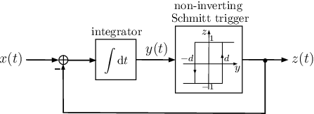
Since its origin, analog-to-digital conversion has been mostly based on uniformly sampling a continuous-time bandlimited signal $x(t)$ at or above the Nyquist rate, followed by a quantization of the samples in amplitude. One thus obtains a digital description from which $x(t)$ is recovered by a one-step sinc interpolation at the precision of quantization. The idea to extend data acquisition to nonuniform sampling has been theoretically studied for quite some time [1, 2, 3, 4, 5] but has attracted relatively low attention in signal processing due to the necessity of complex digital postprocessing. This topic has known revived interest with the recent trend of event-based signal processing [6, 7]. The main motivations behind this movement has been the higher demand for low power and low complexity acquisition devices, while digital postprocessing is becoming more accessible. On the technical side, a main direction of research has been the extraction of samples by time detection of the input’s crossings with fixed amplitude levels, rather than by amplitude measurement of the input at fixed instants [8, 9]. One goal is to boost the overall performance of the acquisition by taking advantage of the inherently higher precision of solid-state circuits in time than in amplitude. A breakthrough in this direction has been the use by Lazar and Tóth of an asynchronous Sigma-Delta modulator (ASDM) [10] (see Fig. 1) to extract level-crossings of the input in the integral domain [11, 12]. This method owes its appeal to the high simplicity of the time encoder, together with the built-in robustness to analog circuit imperfections inherited from Sigma-Delta modulation [13]. This gives the perspective of high-precision low-power acquisition devices, up to remote or offline digital postprocessing. This has given higher motivations to reinvest in the difficult theoretical and practical problem of signal recovery from nonuniform samples. Initial reconstruction methods from time-encoded integrals have been proposed by Lazar and Tóth in [11, 14] for bandlimited inputs, and more recently in [15, 16] for inputs with finite rate of innovation. In this paper, we propose to revisit the reconstruction of bandlimited signals in this problem, all the way from theoretical foundations to real time implementations.

The first part of this paper is to reinterpret the method of [11] from a higher level perspective of nonuniform sampling, and point some fundamental limitations that we address with a new approach. The initial step is to formalize at the most abstract level the knowledge provided by the output of an ASDM about its bandlimited input $x(t)$. We show that this knowledge is a sequence of samples of the form

where ${\sf Z}\subset{\mathbb{Z}}$ and $\langle\cdot,\cdot\rangle$ is the inner-product of $L^{2}({\mathbb{R}})$. The functions $(f_{i}(t))_{i\in{\sf Z}}$ are specifically the bandlimited versions of the rectangular functions $(\pi_{i}(t))_{i\in{\sf Z}}$ shown in Fig. 1 delimited by the switching instants $(t_{i})_{i\in{\sf Z}}$ of the ASDM’s output. The reconstruction of $x(t)$ proposed in [11] can be presented as iterating estimates $x^{\scriptscriptstyle(n)}(t)$ of the form

where $(g_{i}(t))_{i\in{\sf Z}}$ is a different family of functions, namely, sinc functions located at the midpoints of the rectangular functions $(\pi_{i}(t))_{i\in{\sf Z}}$. This choice of functions $g_{i}(t)$ may appear peculiar but was based on an algorithm previously devised in [3] that was proved to converge to $x(t)$ provided that ${\sf Z}={\mathbb{Z}}$ and the switching steps $T_{i}:=t_{i}-t_{i-1}$ for $i\in{\mathbb{Z}}$ have an upper bound $T_{\mathrm{m}}$ smaller than the Nyquist period $T$. However, we indicate in this paper that this sampling condition is not necessary for $x(t)$ to be theoretically and uniquely recoverable from (1). Our first contribution is to propose the alternative choice

where $\|\cdot\|$ is the $L^{2}$-norm. Making $g_{i}(t)$ proportional to $f_{i}(t)$ in (2) appears to be a more legitimate choice as (1) uniquely characterizes its input $x(t)$ basically when the functions $f_{i}(t)$ span the whole considered space ${\mathcal{B}}$ of bandlimited signals. But the precise features and advantages of our method are as follows.

1. The algorithm we use to obtain estimates of the form (2) with (3) is specifically a method of projection onto convex sets (POCS) [17, 18], which is convergent with no condition whatsoever. Their limit $x_{\mathbf{s}}(t)$ is automatically equal to $x(t)$ whenever the samples $(\mathrm{s}_{i})_{i\in{\sf Z}}$ from (1) are uniquely characteristic of $x(t)$.

2. The reconstruction algorithm of [3] used in [11] not only requires the condition $T_{\mathrm{m}}<T$, but also depends on mathematics that are specific to $(\pi_{i}(t))_{i\in{\sf Z}}$ as rectangular functions. Meanwhile, not only does the POCS method require no condition in the present application, but it is a generic algorithm of set theoretic estimation with more powerful properties of convergence, and a wider range of configurations. The present algorithm actually works with any family of functions $(\pi_{i}(t))_{i\in{\sf Z}}$ that is orthogonal in $L^{2}({\mathbb{R}})$. It can therefore be extended to more general schemes of nonuniform sampling, such as integrate-and-fire with leakage [19]. The flexible use of the POCS method has also been anticipated in the recent and independent work of [20, 21] in multi-channel time encoding, for its ability to deal with multiple systems of equations of the type (1). In the present paper, we use another degree of freedom offered by this method, which is the injection of relaxation coefficients in the iteration. This simultaneously permits an acceleration of the convergence, and a computational simplification of significant impact for circuit implementations, as will be seen in the practical contributions of the paper.

3. When there exist more than one bandlimited solution $u(t)$ to the system of equations $\mathrm{s}_{i}=\langle f_{i},u\rangle$ with $i\in{\sf Z}$, then $x_{\mathbf{s}}(t)$ is precisely the solution $u(t)$ that minimizes the $L^{2}$-norm. This type of reconstruction was previously introduced in [22, §III.B.2] in the case of shift-invariant generalized sampling, but also earlier in [2] in the basic case of bandlimited signals with a finite number of samples. Under theoretical conditions that are at least realized by default when ${\sf Z}$ is finite, $x_{\mathbf{s}}(t)$ is more precisely the result of pseudo-inversion of the linear operator

on the sequence $(\mathrm{s}_{i})_{i\in{\sf Z}}$ [23]. This operation is a basic reflex in linear algebra when looking at (1) as the linear equation $Sx=(\mathrm{s}_{i})_{i\in{\sf Z}}$ with possibly many solutions. But the powerful result is that the POCS method of this paper persistently converges to the pseudo-inverse in the more general situation where this equation is inconsistent, due to data noise for example.

4. Theoretical results on perfect reconstruction of bandlimited signals such as Shannon sampling theorem or the result of nonuniform sampling of [3] used in [11] can only work with ${\sf Z}={\mathbb{Z}}$. Meanwhile, the minimal-norm reconstruction $x_{\mathbf{s}}(t)$ is well defined in all cases, including in the practical cases where ${\sf Z}$ is systematically finite. Evidently, one cannot theoretically obtain $x_{\mathbf{s}}(t)=x(t)$ in this situation. But, under a high enough density of samples inside the window of acquisition, $x_{\mathbf{s}}(t)$ is expected to deviate from $x(t)$ only close to the boundaries of this window, in a way similar to the deviations one expects to obtain when truncating the Shannon sampling reconstruction formula. Now, these artifacts are usually ignored in practice as the size of ${\sf Z}$ is typically virtually infinite compared to instantaneous processing windows.

The second contribution of this paper is to propose a practical discrete-time implementation of the algorithm. While the POCS method is originally built in the space of continuous-time signals, a pure discrete-time iteration can be obtained by finding a recursive computation of the coefficients $(\mathrm{c}_{i}^{\scriptscriptstyle(n)})_{i\in{\sf Z}}$ of (2). Such a computation was proposed in [11] involving matrix multiplications of the size of the total signal. Although finite, this size is however virtually infinite compared to the practical windows of operation. For practical implementation, Lazar and Tóth later abandoned their iterative approach and replaced it by a direct block-based resolution of equation (1) [14], following some previously developed method in nonuniform point sampling [24]. This implies the local algebraic pseudo-inversion of matrices within blocks of signals. As a drawback however, this method creates analytically uncontrolled signal distortions at the block boundaries [24], necessitates ad-hoc and empirical methods of compensations, and remains away from traditional pipeline signal processing.

In this paper, we keep the original goal of a recursive computation of $(\mathrm{c}_{i}^{\scriptscriptstyle(n)})_{i\in{\sf Z}}$ and propose its approximate implementation by time-varying FIR filtering. Due to the sampling nonuniformity, the matrices of this computation do not have the convolutional (Toeplitz) structure expected in traditional signal processing. However, the intrinsic decay of sinc functions allows to truncate these matrices along subdiagonals that are away enough from the main diagonal, thus permitting time-varying sliding-window processing. While the approach of [14] is to perform exact algebraic inversions on distorted signals, we return to the traditional signal processing approach, which is on the contrary to preserve the virtually infinite streams of signals while approximating the filtering operators. A similar approach to nonuniform sampling can be found in [25] in the basic case of point sampling, also with the use of a time-varying FIR reconstruction filter. Contrary to the present paper, this work is non-iterative and involves matrix inversions, but these algebraic manipulations are solely used to approximate the filter. The price to pay however is the inversion of one matrix per sample, of the size of the FIR filter.

With the freedom of relaxation allowed by the POCS method, the discrete-time signals that are processed by our FIR filters can be moreover reduced to mere sequences of signed powers of 2. This permits the replacement of every multiplier of the digital implementation by bit shifters, thus significantly reducing complexity and power consumption [26]. Paradoxically, this implementation simplification leads to faster convergence than the plain POCS iteration.

Our method is also suggesting a new framework of nonuniform discrete manipulation of bandlimited signals. Typical digital processing from nonuniform samples such as in [25, 27] tends to unavoidably reconnect with uniform sampling. This prevents or makes difficult a processing that is adaptive and homogeneous with the local density or the irregularity of the samples. Once minimal-norm reconstruction has been adopted as the goal, all working estimates become limited to the subspace of bandlimited signals

which designates the closed linear span of $(f_{i})_{i\in{\sf Z}}$, as can be seen in (2) with (3). In this space, every signal has a discrete expansion of the type (2) (at least when ${\sf Z}$ is finite, and more generally when $S$ has a closed range), where the coefficients $(\mathrm{c}_{i})_{i\in{\sf Z}}$ are in one-to-one correspondence with the nonuniform samples $(\mathrm{s}_{i})_{i\in{\sf Z}}$. The DSP involved in our reconstruction and symbolized in Fig. 2 manipulates these coefficients without any recourse to Nyquist sampling descriptions. In practice, this enables a natural flexible adaptation of the processing with the irregularity of the samples. In theory, this extends DSP to nonuniform discrete descriptions of bandlimited signals.

After reviewing the method of [11] in Section II and its limitation, we present our POCS method in Section III, its unconditional convergence to the minimal-norm bandlimited reconstruction and its connection to pseudo-inversion. In Section IV, we introduce relaxation coefficients into the algorithm and show experimental results of reconstruction in comparison with the method of [11]. In Section V, we transform the iterative part of the algorithm into pure discrete-time computation and exploit the relaxation coefficients to make this free of multipliers, assuming that the inner-products $\langle f_{i},f_{j}\rangle$ are available. By neglecting the small terms in this computation, we show in Section VI a real-time pipeline implementation of it using time-varying FIR filters, and the consequence of the approximations on the reconstruction results, including time quantization. We then show in Section VII how the inner-products $\langle f_{i},f_{j}\rangle$ can be obtained from the sampling steps $(T_{i})_{i\in{\sf Z}}$ by table lookup and some extra additions. While the overall behavior of the POCS algorithm towards noise is that of pseudo-inversion, we finally give in Section VIII some early insight on how the error of the iterates moves from the noise-free algorithmic error to the pure noise-induced error.

The time encoding of a signal $x(t)$ of ${\mathcal{B}}$ as proposed in [11] consists in feeding it into an ASDM as shown in Fig. 1 and recording the successive instants $\tau_{i}$ when the output $z(t)$ switches between $+1$ and $-1$. It is shown in [11] that

where $\pm d$ are the thresholds of the Schmitt trigger. The integral value dependence with the circuit parameter $d$ can be eliminated by considering only the integrals of $x(t)$ between the even-indexed instants $\tau_{2i}$. Defining

one easily obtains from (6) the relation

Here, ${\sf Z}$ denotes either ${\mathbb{Z}}$ or a finite index set $\{1,\cdots,N\}$. This can be formally rewritten as

where

and $1_{I}(t)$ designates the indicator function of any given interval $I$ of ${\mathbb{R}}$. The remaining impact of the parameter $d$ is however in the density of the instants $t_{i}$. For certain mathematical orientations, it will be convenient to have an equivalent expression of (9) that involves only bandlimited functions. Let us define

where $\mathrm{sinc}(t):=\sin(\pi t)/(\pi t)$ and $*$ designates convolution. By even symmetry of the sinc function, we have $\langle\pi_{i},{\mathrm{sinc}*u}\rangle=\langle\mathrm{sinc}*\pi_{i},u\rangle$. Hence,

Then, (9) is equivalent to (1). Depending on the context, we will preferably refer to (1) or to (9).

To reconstruct the signal $x=x(t)$ from ${\mathbf{s}}=(\mathrm{s}_{i})_{i\in{\sf Z}}$, [11] proposes an iteration of the type

where for any $u\in{\mathcal{B}}$,

and $(g_{i})_{i\in{\sf Z}}$ is some family of ${\mathcal{B}}$ to be chosen. Note that any signal $x_{0}$ in the solution space

is a fixed point of (13) given the identity of (12). One way to make (13) convergent is to design $R_{\mathbf{s}}$ so that it is a contraction. When this is possible, ${\mathscr{S}}_{\mathbf{s}}$ is by necessity reduced to a single element, which is $x(t)$, and $x^{\scriptscriptstyle(n)}(t)$ automatically converges to this signal. In this way, one simultaneously proves uniqueness of reconstruction and provides an algorithm that recovers $x(t)$. It is easy to see that

where

For any $x_{0}\in{\mathscr{S}}_{\mathbf{s}}$, one has

The transformation $R_{\mathbf{s}}$ is a contraction when $\|M\|<1$, where $\|\cdot\|$ is here the operator norm in ${\mathcal{B}}$.

Based on some prior results on frames [3, $\lx@sectionsign 8.4$], the work of [11] adopts the following functions

By adapting the derivations of [3]¹¹ 1 While [11] assumes that $\bar{t}_{i}$ is the midpoint of $(t_{i-1},t_{i})$, [3] assumes that $t_{i}$ is the midpoint of $(\bar{t}_{i},\bar{t}_{i+1})$ with $T_{\mathrm{m}}:=\sup_{i\in{\sf Z}}\,(\bar{t}_{i}-\bar{t}_{i-1})$., it is shown in [11, Lemma 3] that $\|M||\leq T_{\mathrm{m}}$ when ${\sf Z}={\mathbb{Z}}$, where

Thus, $M$ is a contraction when

With the circuit parameters of Fig. 1, it is shown in [11] that $T_{\mathrm{m}}\leq 2d/(1{-}x_{\mathrm{m}})$ where $x_{\mathrm{m}}$ is the maximum amplitude of $x(t)$. So $T_{\mathrm{m}}<1$ is guaranteed by choosing $d<(1{-}x_{\mathrm{m}})/2$.

Two pending questions arise from the approach of [11]: (i) $T_{\mathrm{m}}<1$ is sufficient to make $M$ a contraction, but is this necessary? (ii) making $M$ a contraction is sufficient to guarantee that (1) yields $x(t)$ as the unique bandlimited solution, but is this necessary?

An example can be found where the answer is negative for both questions. Consider the case where

for some constant $\delta\in[0,{\frac{1}{2}})$. The sampling here is only periodically nonuniform of period 2. Note that the average density of the instants $(t_{i})_{i\in{\mathbb{Z}}}$ is 1 while $T_{\mathrm{m}}=1+2\delta$. By Fourier analysis, we show in Appendix -A that (1) uniquely characterizes $x(t)$ with any $\delta\in[0,{\frac{1}{2}})$, thus allowing any value of $T_{\mathrm{m}}<2$. Meanwhile, we find that $\|M\|>1$ as soon as $T_{\mathrm{m}}>1.72$. This shows that there are cases where uniqueness of reconstruction is realized with $T_{\mathrm{m}}>1$ while the algorithm of [11] is not guaranteed to converge. Qualitatively speaking, the iteration (13) with the choice of functions $(g_{i})_{i\in{\sf Z}}$ of (19) is not optimally connected to the property of unique reconstruction of $x(t)$ from (1).

Section II-B gave a sufficient but not necessary condition for (1) to uniquely characterize $x(t)$ via the existence of a contractive mapping. As uniqueness of reconstruction lies exactly in the property that ${\mathscr{S}}_{\mathbf{s}}$ defined in (15) is a singleton, we wish to get more insight on the structure of this set.

Finding the exact condition for $(f_{i})_{i\in{\sf Z}}$ to span the whole space ${\mathcal{B}}$ is a difficult theoretical question that goes beyond the scope of this paper. Our goal is at least to estimate $x(t)$ with some element $x_{\mathbf{s}}(t)$ of $S_{\mathbf{s}}$. This will guarantee that $x_{\mathbf{s}}(t)=x(t)$ whenever $(f_{i})_{i\in{\sf Z}}$ effectively spans the whole space ${\mathcal{B}}$ independently of one’s ability to prove it or not. As mentioned in the introduction, the estimate that turns out to be picked by the POCS method is

Note from (23) that ${\mathscr{S}}_{\mathbf{s}}$ is an affine subspace that is closed (even when ${\sf Z}$ is infinite), so its minimal-norm element $x_{\mathbf{s}}(t)$ always exists and is unique. Before we proceed to the description of the reconstruction method, here are some outstanding properties of $x_{\mathbf{s}}(t)$.

These are basic results of linear algebra that can be found in [28] in finite dimension, or in [29] in the context of bounded operators. The above claims are however valid in any Hilbert space without any assumption on the family $(f_{i})_{i\in{\sf Z}}$, as elementary consequences of the Pythagorean theorem. We recall their justification in Appendix -B.

All of the above arguments were solely based on the sampling description of (1) without any assumption on $(f_{i}(t))_{i\in{\sf Z}}$. What will make the POCS method an attractive candidate for signal reconstruction is the particular feature from (11) that $(f_{i}(t))_{i\in{\sf Z}}$ are the bandlimited versions of $(\pi_{i}(t))_{i\in{\sf Z}}$ which form an orthogonal family in $L^{2}({\mathbb{R}})$. In fact, at the exception of Section VII and all experimental results, all the upcoming derivations remain valid with any family $(\pi_{i}(t))_{i\in{\sf Z}}$ that is orthogonal. We recall from the introduction that other applications such as integrate-and-fire with leakage [19] can benefit from this generalization. Given the identity (12), we have the following equivalent description of ${\mathscr{S}}_{\mathbf{s}}$,

where

As both ${\mathcal{B}}$ and ${\Pi_{\mathbf{s}}}$ are closed affine subspaces of $L^{2}({\mathbb{R}})$ (${\Pi_{\mathbf{s}}}$ being the intersection of hyperplanes), the POCS method consists in the following recursion

where $P_{\mathcal{B}}$ and $P_{\Pi_{\mathbf{s}}}$ are the orthogonal projections onto ${\mathcal{B}}$ and ${\Pi_{\mathbf{s}}}$, respectively. This converges to the orthogonal projection of the initial estimate $x^{\scriptscriptstyle(0)}(t)$ onto ${\Pi_{\mathbf{s}}}\cap{\mathcal{B}}$ [18]. When $x^{\scriptscriptstyle(0)}(t)$ is set as the 0 signal, then $x^{\scriptscriptstyle(n)}(t)$ tends to the element of $\Pi_{\mathbf{s}}\cap{\mathcal{B}}$ that is closest to 0 with respect to the $L^{2}$-norm. This is precisely $x_{\mathbf{s}}(t)$ due to (25). Now, by orthogonality of $(\pi_{i}(t))_{i\in{\sf Z}}$, we have explicitly

Thus,

where $R_{\mathbf{s}}$ is defined in (14) with the new functions

This is the choice of functions $g_{i}(t)$ we introduced in (3). We assume from now on this definition of $g_{i}(t)$. As $x^{\scriptscriptstyle(0)}(t)=0$, it is clear from (26) that $x^{\scriptscriptstyle(n)}(t)$ remains in ${\mathcal{B}}$. We have thus established the following result.

In the introduction, we alternatively presented the minimum-norm reconstruction $x_{\mathbf{s}}(t)$ as a result of pseudo-inversion of an operator. This however requires some rigorous mathematical construction that we perform in this section. Consider the space of sequences

This is a Hilbert space equipped with the inner-product

and the induced norm $\|{\mathbf{c}}\|_{\scriptscriptstyle{\mathcal{D}}}:=\langle{\mathbf{c}},{\mathbf{c}}\rangle_{\scriptscriptstyle{\mathcal{D}}}^{1\!/2}$. Then, the mapping $S$ of (4) is rigorously a linear operator of Hilbert spaces

Indeed, due to the identity (12) and the orthonormality of $(\pi_{i}/\|\pi_{i}\|)_{i\in{\sf Z}}$, we have for all $u\in{\mathcal{B}}$,

by Bessel’s inequality, which implies that $Su\in{\mathcal{D}}$. At this occasion, we are finding that $S$ is a bounded operator of norm $\|S\|\leq 1$. With operator notation, equations (1) and (15) then take the form

Let us now define the reconstruction operator

We use the notation $S^{*}$ because this is precisely the adjoint of $S$ given the definition (3) of $g_{i}(t)$. This is seen as follows. For any $u\in{\mathcal{B}}$ and ${\mathbf{c}}\in{\mathcal{D}}$, we have

using the linearity of $\langle\cdot,\cdot\rangle$ with respect to its first argument and (3). Thus $\langle Su,{\mathbf{c}}\rangle_{\scriptscriptstyle{\mathcal{D}}}=\langle u,S^{*}{\mathbf{c}}\rangle$ according to (31), which proves that $S^{*}$ is indeed the adjoint of $S$.

With (12), the transformations $R_{\mathbf{s}}$ and $M$ of (14) and (17) then yield for $u\in{\mathcal{B}}$ the expressions

Given the equation ${\mathbf{s}}=Sx$ of (30), one naturally thinks of invoking the pseudo-inverse $S^{\dagger}$ of $S$ to estimate $x(t)$ from ${\mathbf{s}}$. In standard mathematics, this operator exists whenever the range of $S$, denoted by $\mathrm{ran}(S)$, is closed [23]. It is defined as

As ${\mathbf{s}}\in\mathrm{ran}(S)$, it is easy to see that ${\mathscr{M}}_{\mathbf{s}}={\mathscr{S}}_{\mathbf{s}}$ (the minimum of $\|Su{-}{\mathbf{s}}\|_{\scriptscriptstyle{\mathcal{D}}}$ being 0) and hence

from (24). But the full action of the pseudo-inverse is when the sample sequence ${\mathbf{s}}$ is corrupted by noise. Assume that one only has access to

where ${\bm{\eta}}$ is some noise sequence. One is left with the corrupted POCS iteration

Because $\mathbf{\hat{s}}$ may no longer be in $\mathrm{ran}(S)$, then ${\mathscr{S}}_{\mathbf{\hat{s}}}$ may be empty and hence $x_{\mathbf{\hat{s}}}(t)$ may not exist. The following result will help analyze this iteration.

For any vector of coefficients ${\bm{\lambda}}=(\lambda_{i})_{i\in{\sf Z}}$, we propose to relax the transformation $R_{\mathbf{s}}$ of (14) as

Then, for a given sequence of vectors ${\bm{\lambda}}^{\scriptscriptstyle(n)}$ in $[0,2]^{\sf Z}$, we consider more generally the iteration

To study the convergence of $x^{\scriptscriptstyle(n)}(t)$, we extract the linear part $M^{\bm{\lambda}}$ of $R_{\mathbf{s}}^{\bm{\lambda}}$. Similarly to (16) and (17), we have $R_{\mathbf{s}}^{\bm{\lambda}}u-R_{\mathbf{s}}^{\bm{\lambda}}v=M^{\bm{\lambda}}(u-v)$ where

Since $x_{\mathbf{s}}$ belongs to ${\mathscr{S}}_{\mathbf{s}}$, it is a fixed point of $R_{\mathbf{s}}^{\bm{\lambda}}$ for any ${\bm{\lambda}}$. So, similarly to (18),

One can see from (39) and (3) that $M^{\bm{\lambda}}$ leaves ${\mathcal{V}}_{f}$ invariant. As $x^{\scriptscriptstyle(0)}(t)=0$, then $x^{\scriptscriptstyle(n)}(t)$ remains again in ${\mathcal{V}}_{f}$. It is therefore sufficient to study $M^{\bm{\lambda}}$ in ${\mathcal{V}}_{f}$. We show in Appendix -C the following result.

This implies a strict decrease of $\|x^{\scriptscriptstyle(n)}\!-x_{\mathbf{s}}\|$ as long as $x^{\scriptscriptstyle(n)}(t)\neq x_{\mathbf{s}}(t)$. This is however not sufficient to imply the convergence of $x^{\scriptscriptstyle(n)}(t)$ to $x_{\mathbf{s}}(t)$. This question is difficult when ${\sf Z}$ is infinite. To obtain a firm result of convergence, we will limit ourselves to the case of interest to us where ${\sf Z}$ is finite. It will also be necessary to assume the stronger condition that the relaxation coefficients remain in an interval of the type $[\epsilon,2{-}\epsilon]$ for some constant $\epsilon>0$ as a classic assumption in the literature [30].

One wishes to have some insight on the dependence of the convergence rate with the relaxation coefficients. Analytically, this amounts to seeing how small $\gamma_{\epsilon}$ can be made in (41) compared to 1, depending on ${\bm{\lambda}}$. Its smallest possible value is in fact the operator norm of $M^{\bm{\lambda}}$ restricted to ${\mathcal{V}}_{f}$. Let us formally define

As the general analysis of $\|M^{\bm{\lambda}}\|$ in terms of $\lambda$ is difficult, one wishes to have at least some idea of this quantity when the components $\lambda_{i}$ of ${\bm{\lambda}}$ are equal to a constant value $\lambda$. For convenience, we will simply write in this case $M^{\bm{\lambda}}=M^{\lambda}$, and the goal is to find

In this situation, (38) coincides with a frame algorithm within ${\mathcal{V}}_{f}$ [1, 31] and the optimization of $\|M^{\lambda}\|$ is classic knowledge. Defining the bounds

we have the following result.

As the settings of this paper are not identical to those of [1, 31] (e.g., ${\mathcal{D}}$ is not $\ell^{2}({\sf Z})$) and the present conditions are weaker (e.g., the frame conditions are not guaranteed when ${\sf Z}$ is infinite and $T_{\mathrm{m}}\geq 1$), we justify this result in Appendix -D by adapting the derivations of these references to the present assumptions.

Since $0\leq A\leq B$ with $B\leq 1$ due to (29), then $\lambda_{\mathrm{m}}\geq 1$. In practice, it is likely that $A<B$, which implies that $\lambda_{\mathrm{m}}>1$. This falls in the case of over-relaxation, which is typically the result of optimal relaxation with parallel projections [32], but derived here by connection to the frame algorithm. In practice, as $A$ and $B$ may not be analytically available, the value of $\lambda$ is to be optimized empirically.

We plot in Fig. 4 experimental results of mean squared error (MSE) $\|x^{\scriptscriptstyle(n)}\!-x\|^{2}$ versus $n$ for various iteration methods, in the case where ${\mathcal{B}}$ is the finite dimensional space of bandlimited functions of Nyquist period 1 and signal period $257$. Given the application of the time encoder as an A/D converter, we express the MSE in terms of the bit resolution of a flash A/D converter yielding the same MSE value under the standard uniform quantization noise model [33], with the simple relation 1 bit $=-6.02$ dB of MSE²² 2 If $b$ is the equivalent bit resolution, the MSE in dB’s is equal to $-6.02\,b+\mathrm{MSE}_{0}$, where MSE₀ is the MSE of a random noise uniformly distributed in amplitude and of same maximum amplitude as the signal that is being acquired.. The samples $\{(t_{i},\mathrm{s}_{i})\}_{i\in{\sf Z}}$ are obtained from the encoding method of Section II-A over one period of an input $x(t)\in{\mathcal{B}}$ whose Nyquist-rate samples are randomly and uniformly drawn in the amplitude interval $[-0.5,0.5]$. We adjust the parameter $d$ of the Schmitt trigger (indicated in Fig. 1) so that the average density of instants $t_{i}$ is around 1.5 per Nyquist period. In this situation, ${\mathscr{S}}_{\mathbf{s}}$ has a unique element and hence $x_{\mathbf{s}}(t)=x(t)$. We start with $x^{\scriptscriptstyle(0)}(t)=0$. The plotted MSE is averaged over 1500 drawn inputs.

As a reference, we show the result of [11] in (a). The plain POCS method shown in (c) appears to be somewhat inferior. However, the result of (a) is outperformed by the POCS method with a constant relaxation coefficient $\lambda=1.3$ as shown in (d). This constant value has been found by trial and error to give the best result for the class of random inputs described above. For reference, we also report in (b) the result of another method from [34, Section V]. This work modifies the sinc functions of (19) by deforming their in-band responses to counteract the in-band distortions of the rectangular functions $\pi_{i}(t)$. This appears to give the best results overall. This technique can however not be applied to the POCS method. Meanwhile, relaxation cannot be used to improve it either (as well as the method of [11]).

We show in Fig. 4 the same experiments with a value $d$ that yields an average density of instants $t_{i}$ close to the Nyquist rate (with an optimal value of $\lambda$ equal to 2 in (d)). The figure shows a degradation of all methods with a maximum 4 bit resolution at the 7th iteration while Fig. 4 shows 13 bits of resolution. We explain this by the impact of oversampling on the switching regularity of the ASDM (note that a constant input gives perfectly uniform switching instants). Meanwhile, the iterative reconstructions converge faster with more uniform samples. Increasing the sampling rate however also increases the computation cost due to a higher amount of data to be processed. We will keep working with the conditions of Fig. 4 in the rest of the paper.

The goal of these experiments has been to show how the POCS method performs compared to the existing methods of [11, 34] and show the potential of relaxation for enhancing its performance. Until now, the relaxation coefficients have been chosen to be constant for reference. But the result of interest to us is the curve (e) of Fig. 4, which uses time-varying coefficients for the sake of implementation simplifications. We present this method in the next section.

With (37) and (3), the relaxed POCS iteration of (38) can be presented as

where

Thus

References

- [1] R. Duffin and A. Schaeffer, “A class of nonharmonic Fourier series,” Transactions of the American Mathematical Society, vol. 72, pp. 341–366, Mar. 1952.
- [2] J. L. Yen, “On nonuniform sampling of bandwidth-limited signals,” IRE Trans. Circ. Theory, vol. CT-3, pp. 251–257, Dec. 1956.
- [3] H. G. Feichtinger and K. Gröchenig, “Theory and practice of irregular sampling,” in Wavelets: Mathematics and Applications (J. Benedetto, ed.), pp. 318–324, Boca Raton: CRC Press, 1994.
- [4] F. Marvasti, Nonuniform Sampling: Theory and Practice. New York: Kluwer, 2001.
- [5] A. Aldroubi and K. Gröchenig, “Nonuniform sampling and reconstruction in shift-invariant spaces,” SIAM review, vol. 43, no. 4, pp. 585–620, 2001.
- [6] D. Gontier and M. Vetterli, “Sampling based on timing: Time encoding machines on shift-invariant subspaces,” Applied and Computational Harmonic Analysis, vol. 36, no. 1, pp. 63 – 78, 2014.
- [7] M. Miśkowicz, Event-Based Control and Signal Processing. Embedded Systems, Boca Raton, FL, USA: CRC Press, 2018.
- [8] N. Sayiner, H. V. Sorensen, and T. R. Viswanathan, “A level-crossing sampling scheme for A/D conversion,” IEEE Transactions on Circuits and Systems II: Analog and Digital Signal Processing, vol. 43, no. 4, pp. 335–339, 1996.
- [9] E. Allier, G. Sicard, L. Fesquet, and M. Renaudin, “A new class of asynchronous A/D converters based on time quantization,” in Ninth International Symposium on Asynchronous Circuits and Systems, 2003. Proceedings., pp. 196–205, IEEE, 2003.
- [10] C. Kikkert and D. Miller, “Asynchronous delta sigma modulation,” in Proc. IREE, vol. 36, pp. 83–88, 1975.
- [11] A. Lazar and L. T. Tóth, “Perfect recovery and sensitivity analysis of time encoded bandlimited signals,” IEEE Trans. Circ. and Syst.-I, vol. 51, pp. 2060–2073, Oct. 2004.
- [12] D. Kościelnik and M. Miśkowicz, “Time-to-digital converters based on event-driven successive charge redistribution: A theoretical approach,” Measurement, vol. 45, no. 10, pp. 2511 – 2528, 2012. Special Volume.
- [13] S. Pavan, R. Schreier, and G. Temes, Understanding Delta-Sigma Data Converters. IEEE Press Series on Microelectronic Systems, Wiley, 2017.
- [14] A. A. Lazar, E. K. Simonyi, and L. T. Toth, “An overcomplete stitching algorithm for time decoding machines,” IEEE Transactions on Circuits and Systems I: Regular Papers, vol. 55, pp. 2619–2630, Oct 2008.
- [15] R. Alexandru and P. L. Dragotti, “Reconstructing classes of non-bandlimited signals from time encoded information,” IEEE Transactions on Signal Processing, vol. 68, pp. 747–763, 2020.
- [16] S. Rudresh, A. J. Kamath, and C. Sekhar Seelamantula, “A time-based sampling framework for finite-rate-of-innovation signals,” in ICASSP 2020 - 2020 IEEE International Conference on Acoustics, Speech and Signal Processing (ICASSP), pp. 5585–5589, 2020.
- [17] P. L. Combettes, “The foundations of set theoretic estimation,” Proceedings of the IEEE, vol. 81, pp. 182–208, Feb 1993.
- [18] H. H. Bauschke and J. M. Borwein, “On projection algorithms for solving convex feasibility problems,” SIAM Rev., vol. 38, no. 3, pp. 367–426, 1996.
- [19] H. G. Feichtinger, J. C. Príncipe, J. L. Romero, A. Singh Alvarado, and G. A. Velasco, “Approximate reconstruction of bandlimited functions for the integrate and fire sampler,” Advances in Computational Mathematics, vol. 36, pp. 67–78, Jan 2012.
- [20] K. Adam, A. Scholefield, and M. Vetterli, “Sampling and reconstruction of bandlimited signals with multi-channel time encoding,” IEEE Transactions on Signal Processing, vol. 68, pp. 1105–1119, 2020.
- [21] K. Adam, A. Scholefield, and M. Vetterli, “Encoding and decoding mixed bandlimited signals using spiking integrate-and-fire neurons,” in ICASSP 2020 - 2020 IEEE International Conference on Acoustics, Speech and Signal Processing (ICASSP), pp. 9264–9268, 2020.
- [22] M. Unser and A. Aldroubi, “A general sampling theory for nonideal acquisition devices,” IEEE Transactions on Signal Processing, vol. 42, no. 11, pp. 2915–2925, 1994.
- [23] D. G. Luenberger, Optimization by vector space methods. John Wiley & Sons, Inc., New York-London-Sydney, 1969.
- [24] T. Strohmer, “Numerical analysis of the nonuniform sampling problem,” J. Comput. Appl. Math., vol. 122, pp. 297–316, Oct. 2000.
- [25] H. Johansson and P. Löwenborg, “Reconstruction of nonuniformly sampled bandlimited signals by means of time-varying discrete-time FIR filters,” EURASIP J. Adv. Signal Process, vol. 2006, pp. 105–105, Jan. 2006.
- [26] A. Chandra and S. Chattopadhyay, “Design of hardware efficient FIR filter: A review of the state-of-the-art approaches,” Engineering Science and Technology, an International Journal, vol. 19, no. 1, pp. 212 – 226, 2016.
- [27] S. Tertinek and C. Vogel, “Reconstruction of nonuniformly sampled bandlimited signals using a differentiator–multiplier cascade,” IEEE Transactions on Circuits and Systems I: Regular Papers, vol. 55, no. 8, pp. 2273–2286, 2008.
- [28] S. Garcia and R. Horn, A Second Course in Linear Algebra. Cambridge Mathematical Textbooks, Cambridge University Press, 2017.
- [29] O. Christensen, Frames and bases. Applied and Numerical Harmonic Analysis, Birkhäuser Boston, Inc., Boston, MA, 2008. An introductory course.
- [30] G. T. Herman, A. Lent, and P. H. Lutz, “Iterative relaxation methods for image reconstruction,” in Proceedings of the 1975 Annual Conference, ACM ’75, (New York, NY, USA), pp. 169–174, ACM, 1975.
- [31] K. Grochenig, “Acceleration of the frame algorithm,” IEEE Transactions on Signal Processing, vol. 41, pp. 3331–3340, Dec 1993.
- [32] H. H. Bauschke, P. L. Combettes, and S. G. Kruk, “Extrapolation algorithm for affine-convex feasibility problems,” Numer. Algorithms, vol. 41, no. 3, pp. 239–274, 2006.
- [33] W. Kester, “Taking the mystery out of the infamous formula,"SNR= 6.02 N + 1.76dB," and why you should care,” Analog Devices Tutorial, MT-001 Rev. A, vol. 10, no. 08, 2009.
- [34] N. T. Thao, “Sliding-window signal reconstruction for time encoding machine,” in 2016 Second International Conference on Event-based Control, Communication, and Signal Processing (EBCCSP), pp. 1–7, June 2016.
- [35] D. Hand and M.-W. Chen, “A non-uniform sampling ADC architecture with embedded alias-free asynchronous filter,” in Global Communications Conference (GLOBECOM), 2012 IEEE, pp. 3707–3712, Dec 2012.
- [36] N.T.Thao, “Event-based data acquisition and reconstruction - Mathematical background,” in Event-Based Control and Signal Processing (M. Miśkowicz, ed.), pp. 379–407, Boca Raton, FL, USA: CRC/Taylor and Francis, 2015.
- [37] H. Choi and D. C. Munson, “Analysis and design of minimax-optimal interpolators,” IEEE Transactions on Signal Processing, vol. 46, pp. 1571–1579, Jun 1998.
- [38] T. Elfving, P. C. Hansen, and T. Nikazad, “Semi-convergence properties of Kaczmarz’s method,” Inverse Problems, vol. 30, no. 5, pp. 055007, 16, 2014.
- [39] G. Landi, E. Loli Piccolomini, and I. Tomba, “A stopping criterion for iterative regularization methods,” Appl. Numer. Math., vol. 106, pp. 53–68, 2016.
- [40] M. Vetterli and J. Kovacevic, Wavelets and Subband Coding. Prentice-Hall signal processing series, Prentice Hall PTR, 1995.
- [41] J. B. Conway, A course in functional analysis, vol. 96 of Graduate Texts in Mathematics. Springer-Verlag, New York, second ed., 1990.