Incremental Clustering Techniques for
Multi-Party Privacy-Preserving Record Linkage
Abstract
Privacy-Preserving Record Linkage (PPRL) supports the integration of sensitive information from multiple datasets, in particular the privacy-preserving matching of records referring to the same entity. PPRL has gained much attention in many application areas, with the most prominent ones in the healthcare domain. PPRL techniques tackle this problem by conducting linkage on masked (encoded) values. Employing PPRL on records from multiple (more than two) parties/sources (multi-party PPRL, MP-PPRL) is an increasingly important but challenging problem that so far has not been sufficiently solved. Existing MP-PPRL approaches are limited to finding only those entities that are present in all parties thereby missing entities that match only in a subset of parties. Furthermore, previous MP-PPRL approaches face substantial scalability limitations due to the need of a large number of comparisons between masked records. We thus propose and evaluate new MP-PPRL approaches that find matches in any subset of parties and still scale to many parties. Our approaches maintain all matches within clusters, where these clusters are incrementally extended or refined by considering records from one party after the other. An empirical evaluation using multiple real datasets ranging from to parties each containing up to million records validates that our protocols are efficient, and significantly outperform existing MP-PPRL approaches in terms of linkage quality and scalability.
Keywords:
Data linkage , privacy , scalability , graph matching , multiple databases , subset matching1 Introduction
With the widespread collection of large-scale person-specific databases by many organizations, multiple large databases (held by different parties) often need to be integrated and linked to identify matching records that correspond to the same real-world entity [1, 2, 3] for viable data mining and analytics applications. The absence of unique entity identifiers across different databases requires using commonly available personal identifying attributes, such as names and addresses, for integrating and linking records from those databases. The values in these quasi-identifiers (QIDs) are often dirty, i.e. contain errors and variations, or they can be missing, which makes the linkage task challenging [4, 5]. In addition, such attributes often contain sensitive personal information about the entities to be linked, and therefore sharing or exchanging such values among different organizations is often prohibited due to privacy and confidentiality concerns [6, 7, 8]. Addressing these challenges, privacy-preserving record linkage (PPRL) has attracted increasing interest over the last two decades [1, 8] and been employed in several real applications.
For example, data from hospitals and clinical registries were linked with data from central cancer registries and from the Australian Bureau of Statistics using PPRL techniques for a study on surgical treatment received by aboriginal and non-aboriginal people with lung cancer [9]. Data from several cantonal and national registries were linked in Switzerland using Bloom filter-based PPRL to investigate long-term consequences of childhood cancer [10]. In 2016, the Interdisciplinary Committee of the International Rare Diseases Research Consortium launched a task team to explore approaches to PPRL for linking several genomic and clinical data sets [11].
Further, the Office for National Statistics (ONS) in the UK established the program ‘Beyond 2011’ to carry out research to study the options for production of population and socio-demographics statistics for England and Wales, by linking anonymous data to ensure that high levels of privacy of data about people are maintained [12]. Another application of PPRL in the domain of national security is to integrate data from law enforcement agencies, Internet service providers, businesses, as well as financial institutions, to enable identifying crime and fraud, or of terrorism suspects [13].
The majority of linkage techniques and frameworks have been developed for linking records from only two databases [8, 14, 15]. It is not trivial to extend existing PPRL techniques to multiple databases by sending the encoded databases from all parties to a Linkage Unit (), where a is an external party that has been used in several existing PPRL approaches for conducting or facilitating the linkage of encoded records sent to it by the database owners [8]. At the , it would then become necessary to determine pair-wise similarities between records and to group similar records into clusters where one cluster is assumed to represent one entity [16]. Only few basic grouping/clustering techniques have been described for multi-database linkage, with each of them having limitations as discussed in detail in Section 6. Such clustering schemes have been studied for general record linkage [16, 17, 18] but have received almost no attention so far for PPRL.
Furthermore, sending all the encoded records from multiple parties to the has privacy risks. For example, with Bloom filter-based encoding [19] (to be described in the next section), the more Bloom filters the receives the more likely it will be able to attack these Bloom filter databases using cryptanalysis attacks because more frequency information will become available that can be exploited [20, 21].
Only few techniques have been developed that can perform multi-party linkage in a privacy-preserving context (i.e. MP-PPRL). The main drawbacks of these small number of existing MP-PPRL approaches are that they either (1) only consider the blocking step to reduce the matching space [22] but not how the matching is done, (2) only support exact matching, which classifies record sets as matches if their masked QIDs are exactly the same [4], (3) are applicable to QIDs of categorical data only (however, linkage using QIDs of string data, such as names and addresses, is required in many real applications [8, 23]), or (4) they do not support subset matching where records that match across subsets of databases also need to be identified in addition to records that match across all databases. The primary challenge of MP-PPRL is the complexity of linkage, which generally is exponential with the number of databases to be linked and their sizes [24]. This challenge multiplies when matching records from any possible subset across databases need to be identified.
Contributions: In this paper, we propose an efficient and scalable MP-PPRL protocol that allows subset matching between multiple large databases using a . -based approaches for PPRL are well suited for efficient linking of multiple large databases for practical applications, as the number of communication steps required among the database owners, as well as the risk of information leakage from a sensitive database to other database owners, are reduced when a is used [8].
We develop two variations of incremental clustering combined with a graph-based linkage for MP-PPRL where clusters of encoded records are iteratively merged and refined such that the output of clusters are the matching sets of records (i.e. each cluster represents a set of matching records that correspond to the same entity). Clustering-based approaches are deemed most suitable for holistic data integration, and have been used in several non-PPRL approaches for scaling data integration to many sources [25, 26]. Compared to greedy mapping [27] (as described in Section 3), our proposed incremental clustering methods perform significantly better in terms of linkage quality.
We use counting Bloom filter-based encoding [24] which has lower risk of privacy leakage as the frequency information available in counting Bloom filters is significantly less than basic Bloom filters [24]. Additionally, the risk of collusion between different parties and the can be reduced in our incremental clustering approach by using different encoding parameters in different iterations, as we discuss in Section 4.2.
We provide a comprehensive evaluation of our proposed approach which shows that it has a quadratic computation complexity in the size and the number of the databases that are linked. This complexity is significantly lower compared to the exponential complexity of existing MP-PPRL approaches [23, 24, 28], as we theoretically and empirically validate in Sections 4 and 5 using large real voter and health datasets.
Outline: In Section 2 we provide the required preliminaries and in Section 3 we describe our protocol for MP-PPRL. We analyze our protocol in terms of complexity, privacy, and linkage quality in Section 4, and validate these analyses through an empirical evaluation in Section 5. We discuss related work in MP-PPRL in Section 6. Finally, we conclude the paper with an outlook to future research directions in Section 7.
2 Preliminaries
In this section, we define the problem of MP-PPRL and describe the preliminaries required for our protocol.
Definition 2.1 (MP-PPRL)
Assume are the owners (parties) of the deduplicated databases , respectively. MP-PPRL allows the parties to determine which of their records match with records in other database(s) with and based on the (masked or encoded) quasi-identifiers (QIDs) of these records. The output of this process is a set of match clusters, where a match cluster contains a maximum of one record from each database and . Each is identified as a set of matching records representing the same real-world entity. The parties do not wish to reveal their actual records with any other party. They however are prepared to disclose to each other, or to an external party (such as a researcher), the actual values of some selected attributes of the record sets that are in to allow further analysis.
We assume that the individual databases do not contain any duplicates (i.e. multiple records about the same patient). Each party performs the necessary pre-processing steps including deduplication to ensure the quality of their own database. Many deduplication techniques have been developed in the literature [4, 29] which can be used for deduplicating individual databases before linking them across different parties (such that there is only one record per entity/patient in a database, and therefore a record in one database can match to only one record in another database).
We also assume that a private blocking, indexing, or filtering technique is being used by the database owners [23, 30, 31, 32]. Such techniques are being used in general linkage and PPRL to reduce the number of comparisons by grouping records according to a certain criteria and limiting the comparison only to the records in the same group [4, 8], or by pruning record pairs/sets that are potential non-matches according to some criteria [32]. Note that blocking is not a focus of our paper, and that we assume that the private blocking technique used by the database owners is secure [1].
Since QIDs that are generally used for linking (e.g. names and addresses) contain personal and sensitive information about individuals, PPRL needs to be conducted on the encoded or masked versions of these QIDs. Any masking (encoding) function can be used in our privacy-preserving linkage protocol to encode attribute values, as long as the same function is used by all database owners to mask their databases into , where . We describe our protocol using the Bloom filter (BF) encoding technique, which is widely used in both research and practical applications of PPRL [8, 33, 34]. We also provide an improved solution for privacy-preservation in the multi-party context using counting Bloom filter (CBF) encoding [24].
Definition 2.2 (BF encoding)
A BF is a bit vector of length bits where all bits are initially set to . independent hash functions, , each with range , are used to map each of the elements in a set into the BF by setting the bit positions with to .

For string matching, the -grams (sub-strings of length ) of QID values (that contain textual data, such as names and addresses) of each record in the databases to be linked , with , are hash-mapped into the BF using independent hash functions [35]. Figure 1 illustrates the encoding of bigrams () of two QID values ‘sarah’ and ‘sara’ into bits long BFs using hash functions. The set of bigrams is first extracted from the string (e.g. {’sa’, ’ar’, ’ra’, ’ah’} for ’sarah’) and then each bigram in the set is hashed using hash functions to set the corresponding two indices in the BF to (e.g. hash-mapping bigram ’sa’ results in setting the and bit positions to ). For numerical data, the neighbouring values (within a certain interval) of QID values are hash-mapped into the BF using hash functions [36, 37]. Collision of hash-mapping occurs (for example, the bigrams ’sa’ and ’ra’ are mapped to the same bit position in Figure 1), which improves privacy of the encoding at the cost of loss in utility due to false positives.
In order to allow fuzzy/approximate matching of masked QIDs to perform record linkage in the presence of typographical errors and variations, the similarity/distance between the encoded values needs to be calculated [4, 8]. The similarity of records masked into BFs can be calculated either distributively across all database owners [23, 38] or by a linkage unit [6, 35]. Any set-based similarity function (such as overlap, Jaccard, and Dice coefficient) [4] can be used to calculate the similarity of pairs or sets (multiple) of BFs. In PPRL, the Dice coefficient has been used for matching of BFs since it is insensitive to many matching zeros (bit positions to which no elements are hash-mapped) in long BFs [35].
Definition 2.3 (Dice coefficient similarity)
The Dice coefficient similarity of () BFs () is:
| (1) |
where is the number of common bit positions that are set to in all BFs (common -bits), and is the number of bit positions set to in (-bits), .
For the example Bloom filter pair shown in Figure 1, the number of common -bits is and the number of -bits in the two Bloom filters are and , respectively, and therefore the Dice coefficient similarity is calculated as .
Definition 2.4 (CBF encoding)
A counting Bloom filter (CBF) is an integer vector of length bits that contains the counts of values in each bit position. Multiple BFs can be summarized into a single CBF , such that , where . is the count value in the bit position of the CBF and provides the value in the bit position of BF . Given BFs (bit vectors) with , the CBF can be generated by applying a vector addition operation between the bit vectors such that .
Theorem 2.1
The Dice coefficient similarity of BFs can be calculated given only their corresponding CBF as:
Proof 2.2
The Dice coefficient similarity of BFs (,, , ) is determined by the sum of -bits () in the denominator of Eq. (1) and the number of common -bits () in all BFs in the nominator of Eq. (1). The number of -bits in a BF is , with . The sum of -bits in all BFs is therefore . The value in a bit position () of the CBF of these BFs is . The sum of values in all bit positions of the CBF is which is equal to . Further, if a bit position () contains in all BFs, i.e. , then . Therefore, the common -bits () that occur in all BFs can be calculated by counting the number of positions where , while the sum of the number of -bits () is calculated by summing the values in all bit positions , .

Figure 2 shows an example of using CBF to calculate the similarity of BFs (, , and ). The CBF contains the aggregated counts from the three BFs. The number of common -bits in all three BFs is because indices in contain the count of , and the total number of -bits in all three BFs is , which is the sum of the counts in . Hence, the Dice coefficient similarity is calculated as . As will be described in Sections 3.3 and 4.2, CBFs provide improved privacy compared to BFs in a multi-party context [24].
3 MP-PPRL Protocol
Our protocol allows the efficient identification of matching records from several (two or more) databases held by different parties. We use an incremental graph-based clustering approach to achieve efficient linking of multiple large databases by reducing the exponential comparison space required by traditional linkage methods [8, 22]. The explosion in the number of record pair comparisons required with increasing number of large databases necessitates a transition from batch to incremental clustering methods, which process one database at a time and typically store only a small subset of the data as potential matching records [39].
Overview: Masked/encoded database records are represented by the vertices in a graph and the similarities between compared records are represented by the edges. As we describe below, the databases are ordered using an ordering function to determine in which order the databases are to be processed for incremental clustering. The aim of incremental clustering is to incrementally cluster/group vertices such that similar records from different databases are grouped into one cluster. Vertices containing similar records are identified by using a similarity function. As we describe in Sections 3.1 and 3.2, we propose two mapping functions that perform clustering by merging and/or splitting vertices in the graph. The final output of our protocol is a cluster graph whose vertices are clusters containing similar records, or vertices containing a single record that is not matched with any other records. Each cluster/vertex in the final cluster graph corresponds to one real-world entity. Records within each cluster can be linked as matches and used for further analysis. In the following we describe our protocol in detail.
Definition 3.1 (Cluster graph)
A cluster graph is a -partite graph that contains a set of non-empty independent sets with containing vertices/nodes, and a set of unordered pairs of vertices each representing an undirected edge between a pair of vertices and such that and with . The vertex can be considered as a cluster containing either a single masked record (singleton) or a set of masked records after merging vertices. An edge represents the similarity between masked records in the two vertices and .
Following Definition 3.1, the records from all databases are represented as vertices in a cluster graph , and they are incrementally clustered such that at the end of our protocol each cluster contains a set of matching records from different parties. During incremental clustering we have to assign records of a newly considered party to the already determined clusters of previously matched parties. In general, new records might be similar to several such clusters so that there is a many-to-many match relationship between the set X of already existing clusters and the set Y of new records as shown in Figure 3 (left-hand side). Our goal, however, is to identify the best one-to-one mapping for such matches (Figure 3 (right-hand side)) since the databases are assumed to be deduplicated, and therefore only one-to-one true mapping can exist between records from different databases.

Such one-to-one mappings between the vertices in can be determined by either (1) a greedy approach or (2) an optimal mapping approach that ensures that each record (vertex) is matched with only the best matching record/records from other parties. Given two lists of (unassigned) vertices and , the greedy approach scans through the vertices in and assigns them to the best matching vertex in that is not yet assigned to any other vertex according to their similarity. The greedy approach is not optimal, because when assigning a vertex to a vertex in only the similarities between and unassigned vertices in are considered while neglecting the similarities of the other vertices in with vertices in . Moreover, similar to the best link grouping method proposed by Kendrick [27] (as described in Section 6), greedy mapping depends on the ordering of the vertices/nodes as they are processed.
In our protocol, we therefore use the optimal mapping approach using the Hungarian algorithm [40], which is a combinatorial algorithm for solving the optimal assignment problem in polynomial time. Given two sets of vertices, and , the algorithm determines the optimal one-to-one mapping by assigning a vertex in to a maximum of one vertex in such that the overall similarity between all assigned vertices is maximized:
Definition 3.2 (Optimal mapping)
Given two sets of vertices, and , along with a similarity function . Identify a bijection such that
| (3) |
is maximized.
An illustrative example of optimal one-to-one mapping is shown in Figure 3. For example, has the highest similarity with of while with the similarity is . With greedy mapping (assuming the order of processing as first and then followed by ), is mapped to and therefore needs to be mapped to , and with . This gives a total summed similarity of (Eq. 3). However, with the optimal one-to-one mapping, is mapped with and with while is still mapped to , resulting in a total similarity value of (which is better than the greedy mapping). If , vertices remain not mapped to any vertices after one-to-one mapping is applied.
The proof of Kuhn-Munkres theorem states that for any matching and any feasible labelling (such as greedy mapping), it holds [40]
| (4) |
where denotes the weight function of an edge. Therefore, is the optimal mapping in terms of maximizing edge weights (similarities in our context). We will experimentally evaluate the greedy as well as the optimal mapping approaches in Section 5.
We three initial steps of our MP-PPRL protocol are:

- 1.
All database owners mask (encode) their database records using the same masking function . This can, for example, be BF encoding, as described in Section 2.
- 2.
To reduce the comparison space, a blocking function is applied on the database records (individually by the database owners) to group similar records into the same block according to some criteria (known as blocking key) [4, 30]. All records that have the same (or a similar) blocking key value (BKV) are grouped into the same block. For example, phonetic-based or multi-bit tree-based blocking can be used as the function [4, 30, 35].
- 3.
The masked records () along with their blocks () are sent to a linkage unit () to conduct the linkage of these masked records using the graph-based incremental clustering approach. At the , the records are processed block by block (i.e. each block is considered as one graph , where contains the union of all , with ).
We propose two different methods for incremental clustering in the graphs : (1) early mapping and (2) late mapping. We first present the steps involved in the incremental clustering approach with early mapping in Section 3.1 and then the late mapping-based approach in Section 3.2. While both approaches incrementally merge records from different parties, they differ in when they apply the one-to-one mapping restriction. With early mapping this restriction is continually observed such that every record is only assigned to a single cluster and the number of records per cluster never exceeds the number of parties. By contrast, late mapping assigns records to all clusters for which a minimum similarity is exceeded so that there may temporarily be overlapping clusters and clusters with several records from the same party. The one-to-one restriction is then enforced at the end of the algorithm in a separate mapping phase. Both approaches have a trade-off between complexity and linkage quality, as we will discuss in Section 4.
As will be detailed in the following two sections, the inputs to the incremental clustering algorithm are: masked databases (with ), the union of blocks from all parties , a similarity function for calculating similarities between vertices in , an ordering function for ordering the databases to be processed, a mapping function for one-to-one mapping between vertices in (early mapping, late mapping, or the naïve greedy mapping), a minimum similarity threshold to connect two vertices in by an edge (if their similarity is at least ), and the minimum subset size (), i.e. the minimum number of records that each final cluster must contain.
The databases need to be ordered using the function for incremental clustering. The ordering can be either (a) random, (b) according to their sizes in descending order so that a smaller number of merging will be required, or (c) depending on their data quality of the respective databases in descending order so that the initial clusters will be of higher quality leading to higher linkage quality [41].
3.1 Early mapping-based clustering
The early mapping-based clustering incrementally adds records in each database to the corresponding vertices in the graph by identifying the one-to-one mapping between vertices and records and then merging them. To achieve the one-to-one mapping we apply the Hungarian algorithm [40] according to Definition 3.2 ensuring that a record from one database is matched to a maximum of one cluster of previously matched records and that clusters in the graph are non-overlapping (i.e. ).
Selecting the optimal cluster to which a record should be added is based on the similarities between two vertices of the cluster graph and a minimum similarity threshold . In other words, two vertices are only merged into one if . The similarity between two singletons can easily be calculated using a similarity function, for example the Dice coefficient similarity, to compare the singletons containing records masked into BFs (as described in Section 2).
The similarity between a cluster that contains more than one record and a singleton consisting of a single masked record can be calculated in several ways, including maximum similarity (single linkage), minimum similarity (complete linkage), or average similarity. We use the average similarity function in this work in order to consider data errors and variations, as well as possible variations of the masking function (such as Bloom filter collisions [19]) while not compromising computational efficiency. We leave studying other similarity functions for our incremental clustering as a future work.
Definition 3.3 (Average similarity)
The average similarity between a cluster and a (masked) record (in a singleton) is
| (5) |
with , , and .
The early mapping-based approach involves iterations to perform one-to-one mapping and merging between records from parties. An overview of our clustering approach with early one-to-one mapping is illustrated for linking databases ( iterations) in Figure 4 and outlined in Algorithm 1. The steps of our protocol with early mapping-based clustering are (continuing after the initial steps (1) to (3)):
- 4.
The conducts linkage of masked records in databases from parties. These databases are ordered (using the function in line 2 in Algorithm 1) for incremental clustering. For each block , the masked records in of the first party are added into a graph as separate vertices (lines 3 to 9 in Algorithm 1). Then the second party ’s masked records are inserted into as separate vertices and the similarities between vertices of the first party and the second party are calculated (lines 10 to 13). If the similarity between two vertices is at least a minimum threshold an edge is created between the corresponding vertices (as shown in Figure 4 for and described in lines 14 and 15 in Algorithm 1).
- 5.
The optimal one-to-one mapping (as defined in Section 2) is applied in every iteration (with ) after edges between the records from party (singletons) and clusters of records from parties to have been added. This optimal mapping connects only two highly matching vertices, complying with the assumption of deduplication. All the edges that are not matching after the optimal mapping are removed from (lines 16 to 19).
Algorithm 1: Early mapping-based incremental clustering (Section 3.1) Input: - : Party ’s BFs along with their BKVs, - : Blocks containing the union of blocks from all parties - : Similarity function - : Ordering function for incremental processing of databases - : One-to-one mapping function - : Minimum similarity threshold to classify record sets - : Minimum subset size, with Output: - : Matching record sets (clusters) 1: // Initialization 2: // Order databases 3: for do: // Iterate blocks 4: // Graph for block 5: for do: // Iterate parties 6: if do: // First party 7: for do: // Iterate records 8: 9: // Add vertices 10: if do: // Other parties 11: for do: // Iterate records 12: for do: // Iterate vertices 13: // Calculate similarity 14: if then: 15: // Add edges 16: // 1-to-1 mapping 17: for do: // Iterate edges 18: if then: 19: // Prune edges 20: for do: // Remaining edges 21: // Merge cluster vertices 22: // Add ’s clusters to 23: for do: // Iterate final clusters 24: if then: // Size at least 25: // Add to 26: return // Output - 6.
The vertices that are connected by an edge are then merged into one (lines 20 and 21), while the vertices that do not have any connecting edge (those that are not matching to any vertices in the other databases) are kept as unclustered vertices.
In our running example shown in Figure 4, the optimal mapping (according to the objective function 3) between records of parties and (based on the similarity values) in the first iteration leads to their respective records and to be merged into a single cluster, while from is not clustered with any vertices from . Similarly, and , and and are merged into clusters.
- 7.
The then proceeds with the masked records in of the next (third) party which are first inserted into as separate vertices (singletons). Then the similarities between these vertices and the clustered vertices and singletons from the previous parties’ masked records are calculated and an edge is created connecting those vertices that have a similarity above the minimum threshold (lines 10 to 15 in Algorithm 1). An optimal one-to-one mapping is then applied again between the vertices from all previous parties and the new singleton vertices of the current party in lines 16 to 19. For example in Figure 4, in iteration 2 the singleton vertex with record of the current party and the clustered vertex containing records of previous parties and , respectively, are merged. Similarly, is merged with the cluster containing and from previous parties, while is merged with , as this gives the optimal mapping (according to Equation 3).
- 8.
The vertices connected by an edge after one-to-one mapping (highly matching vertices) at an iteration are merged into one, while the vertices (both clustered and singletons) that are not matching to any other vertices remain as unclustered vertices (lines 20 and 21). For example, the vertex with record of party and the clustered vertex containing records of parties and , respectively, are not merged with any other vertices in iteration 2, as shown in Figure 4.
- 9.
This process of mapping and merging of vertices is repeated until the masked records of all parties are processed (i.e. iterations for each block). The output will be clusters (final vertices in graph ) that either have records from all parties, or a subset of parties, or only one record from a single party. The final clusters of block (i.e. vertices in graph ) are added to (line 22). Based on the minimum subset size required by the MP-PPRL protocol, all the vertices that have a size of at least (i.e. vertices containing matching records from at least parties) are added to the final matching set of records (lines 23 to 26). For example, if in our running example, then will contain only three clusters which are , , and .

| Algorithm 2: Late mapping-based incremental clustering (Section 3.2) | ||
|---|---|---|
| Input: | ||
| - | : Party ’s BFs along with their BKVs, | |
| - | : Blocks containing the union of blocks from all parties | |
| - | : Similarity function | |
| - | : Ordering function for incremental processing of databases | |
| - | : One-to-one mapping function | |
| - | : Minimum similarity threshold to classify record sets | |
| - | : Minimum subset size, with | |
| Output: | ||
| - | : Matching record sets (clusters) | |
| 1: | // Initialization | |
| 2: | for do: | // Iterate blocks |
| 3: | // Graph for block | |
| 4: | for do: | // Iterate parties |
| 5: | if do: | // First party |
| 6: | for do: | // Iterate records |
| 7: | ||
| 8: | // Add vertices | |
| 9: | if do: | // Other parties |
| 10: | for do: | // Iterate records |
| 11: | for do: | // Iterate vertices |
| 12: | // Calculate similarity | |
| 13: | if then: | |
| 14: | // Add edges | |
| 15: | for do: | // Iterate edges |
| 16: | // Merge cluster vertices | |
| 17: | // Order databases | |
| 18: | for do: | // Iterate parties |
| 19: | // Split this party’s records | |
| 20: | // 1-to-1 mapping | |
| 21: | for do: | |
| 22: | // Merge cluster vertices | |
| 23: | // Add ’s clusters to | |
| 24: | for do: | // Iterate final clusters |
| 25: | if then: | // Size at least |
| 26: | // Add to | |
| 27: | return | // Output |
3.2 Late mapping-based clustering
The early mapping-based approach (described in the previous section) is efficient in terms of the number of comparisons required, as we will discuss in Section 4. However, since the optimal mapping is conducted between the records of a database and only the records from the previously processed databases, early mapping can potentially lead to a reduction of the quality of the final linkage results. In this section, we propose a late mapping-based approach to improve linkage quality at the cost of more comparisons.
In addition to one-to-one mapping and merging vertices (as described for the early mapping approach in the previous section), the late mapping approach involves a third phase, which is splitting vertices.
Splitting vertices: Records that belong to a database in a cluster are split into singletons containing the records , while the remaining records from other databases are kept in (with and ).
We next describe the steps of late mapping-based clustering (continuing after the initial steps (1) to (3)). It requires iterations first to merge records from parties, and then iterations for splitting and applying one-to-one mapping, as illustrated in Figure 5 and outlined in Algorithm 2.
- 4.
For each block , the masked records in of the first party () (in any order) are added into a graph as separate vertices (lines 2 to 8 in Algorithm 2). Then the second party ’s masked records are inserted into the graph as separate vertices and the similarities between these singleton vertices of and are calculated (lines 9 to 12). If the similarity between two vertices is at least , then an edge is created between them (as shown in Figure 5 and described in lines 13 and 14 in Algorithm 2).
- 5.
This leads to several many-to-many matched vertices between the two parties, and , since no early optimal mapping is applied. The vertices that are connected by an edge are then merged into one cluster (lines 15 and 16), while the vertices that do not have any connecting edge (those that are not matching to any vertices in the other database) are kept as unclustered vertices.
- 6.
The then proceeds with the masked records of the remaining parties, where the records are first added in as singleton vertices, and then the similarities between these singletons and the clusters from all previous parties’ masked records are calculated and an edge is created connecting those vertices that have a similarity of at least the minimum threshold (lines 9 to 14). The vertices connected by an edge are merged into one (lines 15 and 16), while the vertices that are not matching to any other vertices remain as unclustered vertices.
- 7.
This process of merging vertices is repeated until the masked records of all parties are processed (i.e. iterations for each block). The output will be clusters that are overlapping, which means a record from one party might be in several clusters (i.e. matching with several sets of records from other parties). In the example shown in Figure 5, the merged clusters are overlapping. For example, is in two clusters and in 3 clusters. Since the databases are deduplicated, a record must be matching only to one set of records from other databases. Therefore a late one-to-one mapping needs to be applied on all clusters.
- 8.
In order to conduct late one-to-one mapping, the parties are ordered using the function (similar to the early mapping approach), and the records of the first party in the ordered list are split from the clusters into singleton vertices (one vertex for each unique record) using the function in lines 17 to 19. In the example in Figure 5, records from party are split from the merged clusters into singletons in iteration 1. The optimal one-to-one mapping is then applied between the singletons and the clusters containing unique sets of records from other parties (lines 20 to 22). The number of edges generated for mapping in each iteration corresponds to the number of clusters that appear before splitting in that iteration. In the running example shown in Figure 5, the number of clusters before iteration 1 is (initial merged clusters) and therefore iteration 1 generates edges between ’s singletons and other parties’ clusters. This results in the first party’s records being clustered with the highly matching set of records from other parties. For example, is mapped and merged with the cluster containing , while is merged with the cluster of records .
The process is repeated for all parties ( iterations) in the ordered list until the set of non-overlapping clusters is obtained. As shown in Figure 5, the set of non-overlapping clusters are generated after 3 iterations of splitting and merging of clusters (with one party’s records at an iteration) for linking databases.
It is important to note that late mapping requires more cluster comparisons than early mapping, as it does not prune edges at an early stage potentially leading to many merged clusters. However, it potentially results in better linkage quality since the late one-to-one mapping considers all parties’ records, unlike in early one-to-one mapping where only the previous parties’ records are considered.

Figure 6: An example of using CBFs generated from two BFs and from two respective parties and using a secure summation protocol for similarity calculation, as described in Section 3.3. - 9.
The final (non-overlapping) clusters of block (i.e. vertices in graph ) are added to (line 23). The final clusters with (i.e. vertices containing matching records from at least parties) are added to the final matching set of records (lines 24 to 27).
3.3 Improving Privacy
Our clustering-based MP-PPRL protocol can be used with any encoding/masking technique, such as BF encoding [19] as used in the example described in Figure 1. BF encoding is one of the widely used methods in PPRL due to its efficiency compared to cryptographic methods and controllable/tunable privacy-accuracy trade-off [8, 19, 34].
However, BFs are susceptible to inference attacks by adversaries as has been shown in several studies [20, 21, 42, 43]. Counting Bloom filter (CBF), a variation of BF (as described in Section 2), provides improved privacy guarantees compared to BF for multi-party PPRL [24]. We therefore adapt the CBF-based approach for our protocol to improve privacy against inference attacks. Instead of all parties sending their records’ BFs to a , they can generate CBFs from the BFs using a secure summation protocol, as shown in Figure 6. For example, in the first iteration the first two parties participate in a secure summation protocol [2] with a and generate CBFs for every pair of BFs.
In the basic secure summation protocol [2], the provides a random vector to the first party, which adds its BF to and sends the summed vector to the second party. The second party then adds its BF to the received sum and sends back the final summed vector to the . The subtracts the random vector from the received sum to generate the CBF . Using the generated CBFs, the calculates the similarities of pairs of BFs from the two parties (Equation 2.1).
In the second iteration the already has the possible matches (clusters) from the first two parties. A secure summation protocol is then used by the first three parties and the to generate CBFs from all matches identified in the first iteration along with every BF from the third party. Note that every iteration requires different BF encoding by the corresponding parties to avoid the learning the new party’s BFs. This is repeated until all parties’ records are compared by the .
As discussed in Section 4.2 in detail, CBFs are less vulnerable to inference attacks. However, they incur memory cost ( for BFs of bits) as well as communication costs. Every iteration requires communication steps in the secure summation protocol (for example, when , the number of communication steps required for secure summation is , as illustrated in Figure 6) to generate the CBFs.
4 Analysis of the Protocol
In this section we analyze our MP-PPRL protocol with regard to complexity, privacy, and linkage quality.
4.1 Complexity Analysis
Assume parties participate in the linkage of their respective databases, each containing records, and blocks are generated by the blocking function, each block containing records. In step (1) of our protocol (as described in Section 3), masking records (with average -grams per record) into BFs of length using hash functions for records is for each party. Blocking the databases in step (2) has computation and communication complexity (assuming blocks) at each party. In step (3), masked records from parties need to be sent to the for conducting the linkage, which is of communication complexity.
The early mapping-based approach for incremental clustering has guaranteed quadratic worst case computation complexity in both and . The worst case (in terms of the number of comparisons required) occurs with early one-to-one mapping in two ways: when merging vertices from a database with the vertices in the graph , (a) no vertices (records) in match with vertices in resulting in additional singleton vertices in every iteration, or (b) every vertex/record in matches with a vertex in resulting in vertices with one additional record in every iteration leading to final vertices containing records. The protocol requires iterations for mapping and merging records from databases in each of the blocks. Generally, comparing records from with vertices in in the worst case is of , with . Therefore, the total worst case complexity is , which is .
The late mapping-based approach has an exponential computation complexity in the worst case scenario assuming each record from a database is matched to all records in all other databases (due to the many-to-many matching), leading to overlapping final clusters each containing records. However, assuming the databases are individually deduplicated (as discussed in Section 2) and an appropriate similarity threshold is used for merging clusters, only a small number of additional clusters ( with ) are generally generated in each iteration ( merged clusters in total). This leads to an average computation complexity of , which is . Therefore, the computation complexity of late mapping in the average case is quadratic in both and .
Overall, our MP-PPRL protocol has a worst-case quadratic computation complexity and a linear communication complexity in the number of records and databases , which are both significantly lower than the exponential complexities of earlier MP-PPRL protocols [23, 24, 28]. Please note that extending existing PPRL techniques (that can link two databases with quadratic complexity) to multi-database linkage requires the additional step of clustering once the pair-wise similarities have been calculated. Investigating other clustering algorithms that have been developed for record linkage [16, 17, 18] in the context of MP-PPRL is subject to future research.
4.2 Privacy Analysis
As with most existing PPRL approaches, we assume that all parties follow the honest-but-curious adversary model [44], where the parties follow the protocol while being curious to find out as much as possible about the other parties’ data by means of inference attacks on masked records or by colluding with other parties [45]. We assume the private blocking technique used (as a black box) does not reveal any sensitive information to any parties, and the blocks generated meet the required privacy guarantees, such that each block contains at least a minimum number () of records [45] or are differentially private [46], to overcome frequency attacks.
In the matching step the parties send their masked records (BFs) to the to conduct the linkage. In order to overcome inference attacks by the on the BFs, the counting Bloom filter (CBF)-based approach (described in Section 3.3) can be applied where the sequentially gets a CBF from the relevant set of parties for each cluster of records. Using the CBF the can calculate cluster similarity as equivalent to calculating cluster similarity using individual BFs [24]. CBFs significantly reduce the risk of inference attack compared to BFs [24]. An inference attack allows an adversary to map a list of known values from a global dataset (e.g. -grams or attribute values from a public telephone directory) to the encoded values (BFs or CBF) using background information (such as frequency) [42, 45]. The only information that can be learned from such an inference attack using a CBF of a set of BFs (summed over parties) is if a bit position in is either or which means it is set to or , respectively, in the BFs of all parties.
Proposition 4.1
The probability of identifying the unencoded (original) values of () individual records (with ) given a single CBF is smaller than the probability of identifying the unencoded values of given individual BFs , .
Proof: Assume the number of original (unencoded) values that can be mapped to a masked BF pattern from an inference attack is . in the worst case, where a one-to-one mapping exists between the masked BF and the original unencoded value of . The probability of identifying the original value given a BF in the worst case scenario is therefore [45]. However, a CBF represents BFs and thus at least (in the worst case) original (unencoded) values, which leads to a maximum of with (when , then ). Hence, .
Further, the collusion-resistant secure summation protocols described in [24, 47] can be used to overcome the risk of collusion among the parties in order to learn about another party’s data. We also use the cryptographic long term key (CLK) encoding [35] as a BF hardening method, where QID values of a record are hash-mapped into a record-level BF. This approach improves privacy against inference attacks by decreasing the probability of suspicion [45].
4.3 Linkage Quality Analysis
Our MP-PPRL protocol allows approximate matching of QID values, in that data errors and variations are taken into account depending upon the minimum similarity threshold used. Further, our protocol allows subset matching by identifying matching records across any subset of databases. This improves the linkage quality of MP-PPRL where records of a single entity can be either in all databases or in a subset of databases only (which is often a realistic scenario in practical applications). To the best of our knowledge, this is the first approach that addresses subset matching for MP-PPRL.
The two proposed methods of early and late one-to-one mapping in the incremental clustering approach have a trade-off between complexity and linkage accuracy. As analyzed in Section 4.1, the early mapping approach has lower computational complexity than the late mapping approach. In the following, we analyze the linkage quality of these two mappings.
Conducting early one-to-one mapping in every iteration before merging clusters significantly reduces the computation complexity (as discussed in Section 4.1). However, this approach might reduce linkage quality, because when conducting optimal one-to-one mapping with ’s records then only the records from the previous parties ( to , with ) are considered. In contrast, the late one-to-one mapping is conducted for each party ’s records considering records from all other parties , with and . Therefore, late mapping can improve linkage quality at the cost of more comparisons.
In addition, the linkage quality of our protocol depends on the blocking and the deduplication techniques applied on each database. The higher the quality of deduplication results the better the one-to-one mapping achieved in our approach will be, leading to higher linkage quality. The parties can also be ordered using different ordering functions considering the known quality of their databases or the quality of deduplication results, such that the best quality database is processed first, as the initial clusters will then be of higher quality leading to higher quality clustering in the later iterations [41].
Similarly, the average similarity function we use adds a masked record to a cluster if its similarity on average is high with all masked records in the cluster. Different similarity functions, such as minimum similarity (known as complete linkage), where a masked record needs to have a high similarity with all masked records in the cluster, or maximum similarity (single linkage), where a masked record needs to have a high similarity with at least one masked record in the cluster, would have different impacts on the linkage quality. We leave investigating the impact of different ordering and similarity functions on the linkage quality and efficiency as a future work.
5 Experimental Evaluation
We empirically evaluate the performance of our MP-PPRL protocol (named as AM-Clus) with the two proposed variations, early mapping (EMap) and late mapping (LMap), as well as the baseline greedy mapping (GMap), in terms of scalability, linkage quality, and privacy. In the following sub-section we first describe the datasets we use in our evaluation. In Section 5.2 we discuss the baseline methods to which we compare our proposed clustering approaches, and in Section 5.3 the evaluation measures we employ in our experiments. In Section 5.4 we then describe our experimental setting, and in Section 5.5 we provide an extensive discussion of the results we obtained in these experiments.
5.1 Datasets
One problem with regard to datasets for evaluating MP-PPRL approaches is that there are no datasets available that are generated from multiple parties. Therefore, the general approach to conduct experiments is using multiple datasets sampled with overlap from a single large dataset. We conducted our experiments on three collections of datasets (including a health dataset):
(1) NCVR: A set of datasets generated based on the North Carolina Voter Registration (NCVR) database (available from https://dl.ncsbe.gov/). We extracted 5,000 to 1,000,000 records for 3, 5, 7, and 10 parties with 25% of matching records across all parties and 25% of matching records across subsets of parties. Note that these datasets are different than the NCVR datasets used for the experimental evaluation conducted in [23, 24] for the MP-PPRL approaches that allow full-set matching only (not subset matching). The difference is that these datasets contain 25% of matching records across any subset (of different sizes) of parties and 25% of matching records across all parties, whereas in the datasets used by [23, 24] 50% of matching records appear across all parties.
We also sampled 10 datasets each containing 10,000 records such that 50% of records are non-matches and 5% of records are true matches across each different subset size of to (), i.e. 45% of records are matching in any 2 datasets while only 5% of records are matching in any 9 out of all 10 datasets. Ground truth is available based on the voter registration identifiers to allow linkage quality evaluation.
We generated another series of datasets for each of the datasets generated above, where we included 20% and 40% synthetically corrupted records into the sets of overlapping/matching records (labelled as ’Corr-20’ and ’Corr-40’ in the plots, respectively) using the GeCo tool [48]. For example, if datasets containing 10,000 records each are linked where 5,000 records are matching across at least 2 of these datasets (minimum subset size is 2 in this example), then 1,000 and 2,000 records from these set of true matches are corrupted, respectively. We applied various corruption functions from the GeCo tool on randomly selected attribute values, including character edit operations (insertions, deletions, substitutions, and transpositions), and optical character recognition and phonetic modifications based on look-up tables and corruption rules [48]. Since the matching records (either one or many in the set chosen randomly) are corrupted, the linkage quality will drop which allows us to evaluate how real data errors impact the linkage quality.
(2) NCVRT: We have downloaded the NCVR database every second month since October 2011 and built a combined temporal database of 26 such datasets (i.e. 26 snapshots) each containing over 5 million records of voters [49]. Voter registration identifiers are unique which provides ground truth for evaluation. This real temporal dataset allows conducting large-scale experiments for MP-PPRL assuming each snapshot corresponds to the dataset from one party ( parties).
(3) NSWE: The third dataset is a real New South Wales (NSW) emergency presentations dataset from Australia. A previous study that evaluated our proposed method on this sensitive data by the Centre for Data Linkage at Curtin University provided the presented results [50]. In this study, subsets of NSWE dataset were extracted for 5 parties each containing more than 700,000 records with no duplicates. These datasets were linked by the Centre for Health Record Linkage in Sydney providing ground truth for the linkage [33].
5.2 Baseline Methods
As reviewed in Section 6, only two MP-PPRL techniques are available for approximate matching of string data using probabilistic data structures [23, 24]. We use these two as the baseline approaches to compare our proposed approach as they are closely related to our work. We name these approaches as AM-BF and AM-CBF for the approximate matching approaches based on BF [23] and CBF [24], respectively.
5.3 Evaluation Measures
We evaluate the complexity (scalability) of linkage using runtime and memory size required for the linkage. The quality of the achieved linkage is measured using the precision, recall, and F-measure, calculated on classified matches and non-matches, that have widely been used in record linkage, information retrieval and data mining [4]. The ground truth is available for all datasets with known labels of true matches/clusters (either from all databases for full set matching or subset () of databases for subset matching). For example, the NCVR-10000 datasets for parties contain , i.e. 2,500, record sets (clusters) as true matches from all parties and , i.e. 2,500, record sets as true matches from any subset () of parties.
Based on the classification of the number of true matching record pairs, TM, from each resulting clusters (either from all or subsets of databases), false matches, FM, and false non-matches, FN, the linkage quality measures are defined as below [4]:
- 1.
Precision: the fraction of record pairs in all clusters classified as matches by the PPRL classifier that are true matches:
- 2.
Recall: the fraction of true matches in clusters that are correctly classified as matches by the classifier:
- 3.
F-measure: harmonic mean of Precision and Recall:
We use the F-measure in our evaluation to allow comparison with related earlier publications. We however note that recent research [51] has identified some problematic issues when the F-measure is used to compare record linkage classifiers at different similarity thresholds. This work is ongoing and there is currently no accepted appropriate new measure that combines precision and recall into one single meaningful value.
In line with other work in PPRL [24, 30, 35], we evaluate privacy using disclosure risk (DR) measures based on the probability of suspicion , i.e. the likelihood a masked (encoded) database record in can be matched with one or several known values in a publicly available global database . The probability of suspicion for a masked record , , is calculated as where is the number of possible matches in to the masked record . We conducted a linkage attack [45] assuming the worst case scenario of , and the BF hash functions are known to the adversary. Based on such a linkage attack, we calculate
- 1.
mean disclosure risk (): the average risk ( ) of any sensitive value in being re-identified [45]
- 2.
marketer disclosure risk (): the proportion of masked records in that match to exactly one masked record in ()


5.4 Experimental Setting
Following earlier BF work in PPRL [6, 23, 35], we set the parameters as BF length , the number of hash functions , and the length of grams (substrings of QIDs) is . Soundex-based phonetic encoding [4] is used as the blocking function. The last name is used as the blocking key for the scalability experiments for the different sizes of NCVR datasets, while a combination of first and last name attributes are used as the blocking key attributes for other experiments on the NCVR and NCVRT datasets due to the large runtime requirement. Using last name as the blocking key results in larger blocks and thus requires longer runtime. However, larger blocks improve privacy against frequency attacks on blocks, which is preferred in privacy-preserving applications [8].
We also used an existing multi-party private blocking function using bit-trees [30] on the surname and date of birth attributes for linking the NSWE datasets. Soundex-based phonetic blocking on first and last names provides an average pairs completeness (similar to recall it calculates the percentage of true matches found in the candidate record sets generated by a blocking method [4]) of and the bit-trees-based blocking on surname and date of birth values provides pairs completeness. We used the first name, last name, city, and zipcode attributes as QIDs for the linkage of the NCVR and NCVRT datasets, while first name, surname, date of birth, sex, address, and postcode are used as QIDs for linking records in the NSWE datasets. These attributes are commonly used personal identifying attributes for linking records across databases [4].
We implemented both our proposed approaches and the competing baseline approaches in Python 2.7.3, and ran all experiments on a server with four 6-core 64-bit Intel Xeon 2.4 GHz CPUs, 128 GBytes of memory and running Ubuntu 14.04. The programs and test datasets (except NSWE) are available from the authors.
5.5 Discussion
In this section we discuss the results of our experimental study.
i. Comparison of different mapping: In Figure 7 (a) we compare the runtime for our approach based on greedy (baseline), early and late mappings (labelled as GMap, EMap and LMap, respectively), while in Figure 7 (b) we compare their F-measure results on the NCVR datasets. The proposed early and late mappings require similar or lower runtime than the baseline greedy mapping, and as expected the F-measure achieved with early and late mappings are significantly higher than greedy mapping. Early mapping requires comparatively lower runtime than late mapping at the cost of a small loss in linkage quality. Since the loss in F-measure is not very significant, we use the early mapping-based approach as a default mapping in the rest of our experiments.


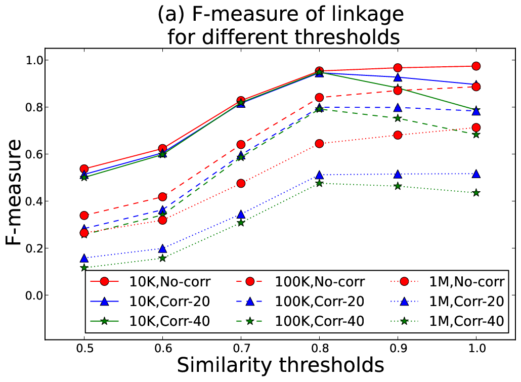
ii. Similarity threshold vs. linkage quality: The F-measure achieved with different similarity thresholds on the NCVR datasets for is shown in Figure 8 (a). The F-measure increases with the threshold up to on all datasets and then drops due to the loss in recall. As can be seen, the F-measure increases with larger thresholds on non-corrupted datasets (which require only exact matching) while it starts to decrease at a certain point on the corrupted datasets (which require approximate matching due to errors and variations). We therefore set the default threshold value to in our experiments. When the datasets are corrupted, the linkage quality becomes very low with increasing dataset sizes. These results indicate that more advanced classification techniques instead of a simple threshold-based classification are required to improve the linkage quality in the presence of real-world data errors [4].


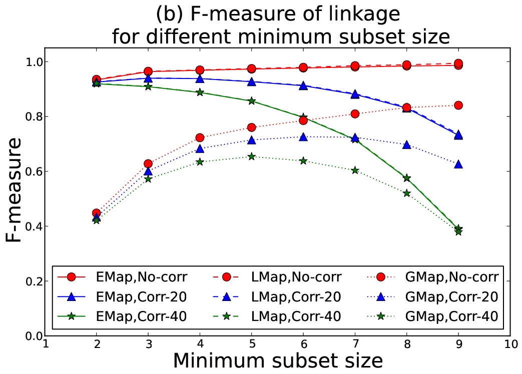
iii. Minimum subset size vs. linkage quality: The F-measure of linkage achieved with different minimum subset sizes on the NCVR datasets for the early, late, and greedy mappings are shown in Figure 8 (b). Linking with smaller minimum subset size is more challenging than larger minimum subset size, as identifying matches across or more datasets is more difficult than all datasets, for example, due to the large number of combinations of datasets to be checked for matches. Our proposed mapping approaches outperform the greedy mapping significantly for smaller minimum subset sizes.
As expected, the linkage becomes more challenging with corrupted data using any mapping methods, when identifying records that match across larger number of databases compared to smaller subsets of databases. With increasing number of databases, more corrupted records are included in the matches, resulting in significant loss of linkage quality. While data errors in real data are possible, the degree of corruption would be probably relatively low. According to the real NSWE and NCVRT datasets, the quality of data is very high with less than 1% linkage errors when a probabilistic two-database matching technique is applied on the unencoded NSWE dataset [52] and around 10% error in the NCVRT dataset. We have tested relatively pessimistic scenarios by synthetically including 20% and 40% corruption to the matching records in NCVR datasets. The results on the corrupted datasets indicate that achieving high linkage quality in the presence of large amount of data errors is a big challenge, which needs to be mitigated through appropriate pre-processing techniques as well as clerical review possibly using active learning techniques [1].
iv. Scalability: We next evaluate the scalability of our protocol for different dataset sizes on the NCVR datasets in Figure 9. When a combination of first and last name (labelled as FName and LName, respectively in the figure) attributes are used as blocking keys (BK), the resulting block sizes become small, making our protocol highly scalable in terms of runtime and memory size to large datasets from multiple parties. However, when only the last name attribute is used as the BK our protocol shows a quadratic trend with the size and number of the datasets. The experiments on larger datasets of 500K and 1M with one attribute as BK required very large runtime due to the larger block sizes, and therefore we did not conduct this set of experiments due to time limitation. Advanced blocking and filtering techniques are therefore required to further reduce the computational complexity of large-scale multi-party linkage.


v. Large-scale linkage: We conducted large-scale experiments of our approach on the NCVRT and NSWE datasets. As can be seen in Figures 10 (a) and (b), we are able to link multiple large datasets and achieve high linkage quality, which shows the viability of our approach for large-scale MP-PPRL applications. Since multi-database linkage requires an additional step of clustering (or mapping) after pair-wise matching, investigating other better clustering techniques that can achieve improved linkage quality is subject to further research. However, as shown in Figure 10 (a), the runtime required for linking such large multiple datasets is higher (even though it is significantly better compared to the baseline methods, as will be discussed below) and therefore more advanced computational methods, such as distributed computing and parallel processing, need to be investigated to further improve the efficiency of MP-PPRL.
vi. Comparison with baseline: We next compare our approach with the baseline approaches in Figure 11 in terms of scalability and linkage quality. As can be seen in Figure 11 (a), our approaches (EMap and LMap) require lower runtime for linking a large number of databases, where the runtime does not increase significantly with compared to AM-BF. The AM-BF approach requires lower runtime for linking smaller number of databases, however it increases exponentially with larger . We were unable to conduct experiments for this approach on the NCVR-100K datasets due to excessive memory consumption with the exponential number of comparisons required by this approach. The AM-CBF approach is more scalable than AM-BF for linking a larger number of databases. This is because the improved communication patterns with CBF reduce the exponential growth with down to the ring size , where [24]. However, our proposed methods require even lower runtime than AM-CBF and is more scalable with increasing .


As shown in Figure 11 (b), our approaches (EMap and LMap) achieve substantially higher F-measure results compared to all baseline methods on both non-corrupted and corrupted datasets by identifying matching records not only across all databases but also across subsets of databases. We also compared the F-measure of all these approximate matching approaches with an exact matching MP-PPRL protocol [28], and as expected the approximate matching approaches outperform it on corrupted datasets.
vii. Disclosure risk results: As shown in Figure 12, the CBF-based masking consistently has lower mean and marketer disclosure risk than BF-based masking (as we discussed in Section 4.2). Therefore, CBF-based masking provides improved privacy than BF-based masking. This means that the same privacy results can be achieved by our protocol in terms of mean and marketer disclosure risks as with other CBF-based approaches [24] in the worst case.
This comparative evaluation shows that our AM-Clus approach outperforms existing approaches in terms of scalability and linkage quality, while providing better/similar privacy results.
6 Related Work
Various techniques have been proposed in the literature tackling the problem of PPRL, as surveyed in [1, 8, 35, 53]. However, most of these approaches are limited to linking only two databases, and only few approaches have considered linking data from multiple databases (MP-PPRL). Neither of these techniques allow subset matching for MP-PPRL where records that match across subsets of databases are also identified in addition to records that match across all databases.
A secure multi-party computation approach using an oblivious transfer protocol was proposed by O’Keefe et al. [54] for PPRL on multiple databases. While provably secure, the approach can only perform exact matching (i.e. variations and errors in the QIDs are not considered). Kantarcioglu et al. [55] introduced a MP-PPRL approach for categorical data to perform secure equi-joins (exact matching) on -anonymous databases, where the QIDs of a record are similar to at least other records in the database [56]. An exact matching approach for categorical data was recently proposed by Karapiperis et al. [7] using a Count-Min sketch data structure. Sketches are used to summarize the local set of elements which are then intersected to provide a global synopsis using homomorphic operations and symmetric noise addition techniques [2, 44]. Another exact matching approach for MP-PPRL using Bloom filter (BF) encoding was introduced by Lai et al. [28], where a conjuncted BF is jointly constructed by all parties to identify matching records.
All the MP-PPRL techniques described above are not practical in real applications as they allow only exact matching or matching of categorical data. Vatsalan and Christen extended Lai et al.’s exact matching approach [28] to develop an approximate matching solution for MP-PPRL [23] by using BFs and a secure summation protocol [2, 44] to distributively calculate the similarity of a set of BFs from different parties. A recent approach for approximate matching in MP-PPRL based on Counting Bloom filter (CBF) was proposed by Vatsalan et al. [24]. BFs from different databases were summarized into a single CBF by applying a secure summation protocol. Neither of these MP-PPRL approaches, however, supports identifying matching records in subset of parties.
Only limited grouping techniques have been developed to identify a set of matching records from multiple databases in the literature. Merge-based grouping simply groups or merges into one set all the records that have a similarity above the threshold [57]. The greedy best link approach proposed by Kendrick [27] links each incoming record to the group that has the highest similarity with the incoming record. An improved version of the best link approach was later proposed by Randall et al. [26], which is referred to as weighted best link. In this approach all the records in the incoming file are first linked with the matching group of records, and then they are amalgamated according to the order of their weights. The advantage of the weighted best link approach is that it does not depend on the order of incoming records. However, the results depend on how the weights are calculated. Our proposed incremental clustering approaches are not only independent of the ordering of records but also the weights of links.
Scalability of PPRL has been addressed through the development of private blocking functions [22, 58, 59], and the more recently proposed summarization algorithms [60]. However, the number of comparisons required for multi-party linkage remains very large even with such existing private blocking and filtering approaches employed [23, 30]. Recent work by Vatsalan et al. [24] proposed improved communication patterns for reducing the number of comparisons for CBF-based MP-PPRL. The naïve computation complexity of MP-PPRL techniques is exponential in the number of records per database (, assuming records in each of the databases). The improved communication patterns developed by Vatsalan et al. [24] reduce this exponential growth with down to the ring size (with ). In contrast, our proposed approach efficiently performs subset matching with a quadratic computation complexity in the size and number of databases (), which allows large-scale MP-PPRL.
7 Conclusion
We have presented a scalable MP-PPRL protocol that is highly efficient for practical applications, such as health data linkage, and it improves the linkage quality compared to existing MP-PPRL approaches that only allow identifying matching records across all databases and do not support subset matching. Our protocol uses graph-based incremental clustering to achieve efficient identification of matching records across all and subsets of large databases.
An experimental evaluation conducted on large real datasets (including 26 voter registration databases each containing over 5 million records and 5 real emergency admissions datasets each containing around 700,000 records) shows that our approach is practical for real large-scale MP-PPRL applications. Our approach outperforms existing MP-PPRL approaches in terms of linkage quality and scalability.
In future work, we aim to investigate how existing clustering algorithms for record linkage [16, 17, 18, 61, 62] can be adapted for MP-PPRL. One important direction of this work is to study incremental clustering for dynamic data matching in MP-PPRL [63]. We also plan to evaluate the impact of pre-processing techniques, especially dealing with missing values [64], on the performance of privacy-preserving clustering. Another direction is to study how incremental clustering can be parallelized to improve scalability of large-scale MP-PPRL. Investigating other advanced mapping, encoding, similarity, and classification functions (including relational clustering and collective classification [4]) for clustering-based MP-PPRL would also be interesting directions for future work.
8 Acknowledgements
This work was partially funded by the Australian Research Council under Discovery Projects DP130101801 and DP160101934, and Universities Australia and the German Academic Exchange Service (DAAD). We would like to thank Sean Randall from the Centre for Data Linkage, Curtin University, for conducting experiments using our proposed methods on the sensitive NSWE dataset.
9 References
References
- [1] D. Vatsalan, Z. Sehili, P. Christen, E. Rahm, Privacy-preserving record linkage for Big data: Current approaches and research challenges, in: Handbook of Big Data Technologies, Springer, 2017, pp. 851–895.
- [2] C. Clifton, M. Kantarcioglu, J. Vaidya, X. Lin, M. Y. Zhu, Tools for privacy preserving distributed data mining, SIGKDD Explorations 4 (2) (2002) 28–34.
- [3] S. L. Cheah, V. L. Scarf, C. Rossiter, C. Thornton, C. S. Homer, Creating the first national linked dataset on perinatal and maternal outcomes in australia: Methods and challenges, Journal of Biomedical Informatics (2019) 103152.
- [4] P. Christen, Data matching - concepts and techniques for record linkage, entity resolution, and duplicate detection, Data-Centric Systems and Applications, Springer, 2012.
- [5] Y. Chi, J. Hong, A. Jurek, W. Liu, D. O’Reilly, Privacy preserving record linkage in the presence of missing values, Information Systems 71 (2017) 199–210.
- [6] E. A. Durham, C. Toth, M. Kuzu, M. Kantarcioglu, Y. Xue, B. Malin, Composite Bloom filters for secure record linkage, IEEE Transactions on Knowledge and Data Engineering 26 (12) (2014) 2956–2968.
- [7] D. Karapiperis, D. Vatsalan, V. S. Verykios, P. Christen, Large-scale multi-party counting set intersection using a space efficient global synopsis, in: Database Systems for Advanced Applications, Hanoi, 2015.
- [8] D. Vatsalan, P. Christen, V. S. Verykios, A taxonomy of privacy-preserving record linkage techniques, Information Systems 38 (6) (2013) 946–969.
- [9] J. R. Condon, T. Barnes, J. Cunningham, B. K. Armstrong, Long-term trends in cancer mortality for indigenous australians in the northern territory, Medical Journal of Australia 180 (10) (2004) 504.
- [10] C. E. Kuehni, C. S. Rueegg, G. Michel, C. E. Rebholz, M.-P. F. Strippoli, F. K. Niggli, M. Egger, N. X. von der Weid, S. P. O. G. (SPOG), Cohort profile: the Swiss childhood cancer survivor study, International journal of epidemiology 41 (6) (2011) 1553–1564.
- [11] D. Baker, B. M. Knoppers, M. Phillips, D. van Enckevort, P. Kaufmann, H. Lochmuller, D. Taruscio, Privacy-preserving linkage of genomic and clinical data sets, IEEE/ACM Transactions on Computational Biology and Bioinformatics (2018) 1.
- [12] Office for National Statistics, Matching anonymous data, in: Beyond 2011, 2013.
- [13] C. Phua, K. Smith-Miles, V. C. Lee, R. Gayler, Resilient identity crime detection, IEEE Transactions on Knowledge and Data Engineering 24 (3) (2012) 533.
- [14] H. Köpcke, E. Rahm, Frameworks for entity matching: A comparison, Data & Knowledge Engineering 69 (2) (2010) 197–210.
- [15] D.-W. Wang, C.-J. Liau, T.-s. Hsu, An epistemic framework for privacy protection in database linking, Data & Knowledge Engineering 61 (1) (2007) 176–205.
- [16] O. Hassanzadeh, F. Chiang, H. C. Lee, R. J. Miller, Framework for evaluating clustering algorithms in duplicate detection, Proceedings of the Very Large Database Endowment 2 (1) (2009) 1282–1293.
- [17] C. Nanayakkara, P. Christen, T. Ranbaduge, Robust temporal graph clustering for group record linkage, in: Pacific-Asia Conference on Knowledge Discovery and Data Mining, Macau, 2019.
- [18] A. Saeedi, M. Nentwig, E. Peukert, E. Rahm, Scalable matching and clustering of entities with famer, Complex Systems Informatics and Modeling Quarterly (16) (2018) 61–83.
- [19] R. Schnell, T. Bachteler, J. Reiher, Privacy-preserving record linkage using Bloom filters, BMC Medical Informatics and Decision Making 9 (1) (2009) 1.
- [20] P. Christen, A. Vidanage, T. Ranbaduge, R. Schnell, Pattern-mining based cryptanalysis of Bloom filters for privacy-preserving record linkage, in: PAKDD, Springer LNAI, Melbourne, 2018, pp. 530–542.
- [21] P. Christen, T. Ranbaduge, D. Vatsalan, R. Schnell, Precise and fast cryptanalysis for Bloom filter based privacy-preserving record linkage, IEEE Transactions on Knowledge and Data Engineering (2018) 1.
- [22] P. Christen, A survey of indexing techniques for scalable record linkage and deduplication, IEEE Transactions on Knowledge and Data Engineering 24 (9) (2012) 1537–1555.
- [23] D. Vatsalan, P. Christen, Scalable privacy-preserving record linkage for multiple databases, in: ACM Conference in Knowledge Management, Shanghai, 2014.
- [24] D. Vatsalan, P. Christen, E. Rahm, Scalable privacy-preserving linking of multiple databases using counting Bloom filters, in: Workshop on Privacy and Discrimination in Data Mining held at IEEE ICDM, Barcelona, 2016.
- [25] E. Rahm, The case for holistic data integration, in: Advances in Databases and Information Systems, Springer, 2016, pp. 11–27.
- [26] S. M. Randall, J. H. Boyd, A. M. Ferrante, A. P. Brown, J. B. Semmens, Grouping methods for ongoing record linkage, in: KDD Workshop on Population Informatics, Sydney, 2015.
- [27] S. Kendrick, M. Douglas, D. Gardner, D. Hucker, Best-link matching of Scottish health data sets., Methods of Information in Medicine 37 (1) (1998) 64–68.
- [28] P. Lai, S.-M. Yiu, K. Chow, C. Chong, L. Hui, An Efficient Bloom filter based Solution for Multiparty Private Matching, in: Security and Management, Las Vegas, 2006.
- [29] F. Naumann, M. Herschel, An introduction to duplicate detection, Synthesis Lectures on Data Management 2 (1).
- [30] T. Ranbaduge, P. Christen, D. Vatsalan, Tree based scalable indexing for multi-party privacy-preserving record linkage, in: Australasian Data Mining, Brisbane, 2014.
- [31] A. Al-Lawati, D. Lee, P. McDaniel, Blocking-aware private record linkage, in: IQIS, 2005, pp. 59–68.
- [32] Z. Sehili, L. Kolb, C. Borgs, R. Schnell, E. Rahm, Privacy preserving record linkage with PPJoin, in: BTW Conference, Hamburg, 2015.
- [33] S. M. Randall, A. M. Ferrante, J. H. Boyd, J. B. Semmens, Privacy-preserving record linkage on large real world datasets, Journal of Biomedical Informatics 50 (1) (2014) 1.
- [34] A. P. Brown, S. M. Randall, J. H. Boyd, A. M. Ferrante, Evaluation of approximate comparison methods on bloom filters for probabilistic linkage, International Journal of Population Data Science 4 (1).
- [35] R. Schnell, Privacy preserving record linkage, in: K. Harron, H. Goldstein, C. Dibben (Eds.), Methodological developments in data linkage, Wiley, Chichester, 2016, pp. 201–225.
- [36] D. Vatsalan, P. Christen, Privacy-preserving matching of similar patients, Journal of Biomedical Informatics 59 (2016) 285–298.
- [37] D. Karapiperis, A. Gkoulalas-Divanis, V. S. Verykios, Distance-aware encoding of numerical values for privacy-preserving record linkage, in: International Conference on Data Engineering, San Diego, 2017, pp. 135–138.
- [38] D. Vatsalan, P. Christen, An iterative two-party protocol for scalable privacy-preserving record linkage, in: Australasian Data Mining Conference, Sydney, 2012.
- [39] M. Ackerman, S. Dasgupta, Incremental clustering: The case for extra clusters, in: Advances in Neural Information Processing Systems, 2014, pp. 307–315.
- [40] H. W. Kuhn, The hungarian method for the assignment problem, Naval research logistics quarterly 2 (1-2) (1955) 83–97.
- [41] M. Nentwig, E. Rahm, Incremental clustering on linked data, in: Workshop on Data Integration and Application held at IEEE ICDM, Singapore, 2018.
- [42] M. Kuzu, M. Kantarcioglu, E. Durham, B. Malin, A constraint satisfaction cryptanalysis of Bloom filters in private record linkage, in: Privacy Enhancing Technologies Symposium, Waterloo, Canada, 2011, pp. 226–245.
- [43] F. Niedermeyer, S. Steinmetzer, M. Kroll, R. Schnell, Cryptanalysis of basic Bloom filters used for privacy preserving record linkage, Journal of Privacy and Confidentiality 6 (2) (2014) 59–79.
- [44] Y. Lindell, B. Pinkas, Secure multiparty computation for privacy-preserving data mining, Journal of Privacy and Confidentiality 1 (1) (2009) 1.
- [45] D. Vatsalan, P. Christen, C. M. O’Keefe, V. S. Verykios, An evaluation framework for privacy-preserving record linkage, Journal of Privacy and Confidentiality 6 (1) (2014) 1.
- [46] M. Kuzu, M. Kantarcioglu, A. Inan, E. Bertino, E. Durham, B. Malin, Efficient privacy-aware record integration, in: ACM International Conference on Extending Database Technology, Genoa, Italy, 2013, pp. 167–178.
- [47] T. Tassa, D. J. Cohen, Anonymization of centralized and distributed social networks by sequential clustering, IEEE Transactions on Knowledge and Data Engineering 25 (2) (2013) 311–324.
- [48] K.-N. Tran, D. Vatsalan, P. Christen, GeCo: an online personal data generator and corruptor, in: ACM Conference in Knowledge Management, San Francisco, 2013, pp. 2473–2476.
- [49] P. Christen, Preparation of a real voter data set for record linkage and duplicate detection research, Tech. rep., Research School of Computer Science, Australian National University (2014).
- [50] T. Ranbaduge, D. Vatsalan, S. Randall, P. Christen, Evaluation of advanced techniques for multi-party privacy-preserving record linkage on real-world health databases, in: International Population Data Linkage Conference, Swansea, Wales, 2016.
- [51] D. Hand, P. Christen, A note on using the F-measure for evaluating record linkage algorithms, Statistics and Computing 28 (3) (2018) 539–547.
- [52] S. Randall, A. Brown, J. Boyd, R. Schnell, C. Borgs, A. Ferrante, Sociodemographic differences in linkage error: an examination of four large-scale datasets, BMC Health Services Research 18 (1) (2018) 678.
- [53] S. Trepetin, Privacy-preserving string comparisons in record linkage systems: a review, Information Security Journal: A Global Perspective 17 (5) (2008) 253–266.
- [54] C. M. O’Keefe, M. Yung, L. Gu, R. Baxter, Privacy-preserving data linkage protocols, in: ACM Workshop on Privacy in the Electronic Society, Washington, 2004.
- [55] M. Kantarcioglu, W. Jiang, B. Malin, A privacy-preserving framework for integrating person-specific databases, in: Privacy in Statistical Databases, Istanbul, 2008, pp. 298–314.
- [56] L. Sweeney, K-anonymity: A model for protecting privacy, International Journal of Uncertainty Fuzziness and Knowledge Based Systems 10 (5) (2002) 557–570.
- [57] S. M. Randall, J. H. Boyd, A. M. Ferrante, J. K. Bauer, J. B. Semmens, Use of graph theory measures to identify errors in record linkage, Computer Methods and Programs in Biomedicine 115 (2) (2014) 55–63.
- [58] T. Ranbaduge, P. Christen, D. Vatsalan, Clustering-based scalable indexing for multi-party privacy-preserving record linkage, in: PAKDD, Springer LNAI, Hanoi, 2015.
- [59] T. Ranbaduge, D. Vatsalan, P. Christen, Hashing-based distributed multi-party blocking for privacy-preserving record linkage, in: PAKDD, Springer LNAI, Auckland, 2016.
- [60] D. Karapiperis, A. Gkoulalas-Divanis, V. S. Verykios, Summarizing and linking electronic health records, Distributed and Parallel Databases (2019) 1–40.
- [61] S. Chakraborty, N. Nagwani, Analysis and study of incremental k-means clustering algorithm, in: High Performance Architecture and Grid Computing, Springer, 2011, pp. 338–341.
- [62] H. Yin, A. R. Benson, J. Leskovec, D. F. Gleich, Local higher-order graph clustering, in: ACM SIGKDD International Conference on Knowledge Discovery and Data Mining, ACM, 2017, pp. 555–564.
- [63] Z. Li, J.-G. Lee, X. Li, J. Han, Incremental clustering for trajectories, in: International Conference on Database Systems for Advanced Applications, Springer, 2010, pp. 32–46.
- [64] I. C. Anindya, M. Kantarcioglu, B. Malin, Determining the impact of missing values on blocking in record linkage, in: PAKDD, Springer LNAI, Macau, 2019, pp. 262–274.